Scalar self-force for eccentric orbits around a Schwarzschild black hole
Abstract
We revisit the problem of computing the self-force on a scalar charge moving along an eccentric geodesic orbit around a Schwarzschild black hole. This work extends previous scalar self-force calculations for circular orbits, which were based on a regular “effective” point-particle source and a full 3D evolution code. We find good agreement between our results and previous calculations based on a (1+1) time-domain code. Finally, our data visualization is unconventional: we plot the self-force through full radial cycles to create “self-force loops”, which reveal many interesting features that are less apparent in standard presentations of eccentric-orbit self-force data.
I Introduction
Gravitational waves from highly relativistic systems such as compact object binaries are of significant interest in astrophysics and fundamental physics. For astrophysics, gravitational waves will eventually complement traditional observations based on electromagnetic waves, by allowing us to peer through otherwise opaque regions of the cosmos [1]. And for fundamental physics, gravitational wave observations can serve as useful tools for probing strong-gravity phenomena, supplementing the existing suite of weak-field, cosmological, and purely theoretical constraints on alternative theories of gravity [2].
One very promising class of highly relativistic systems are binaries consisting of a massive black hole (say of mass ) and a solar-mass compact object (of mass ), where . These are known as EMRIs [2, 3] — short for extreme-mass-ratio inspirals — because of their general inspiraling behavior and the very small ratio () between the constituent masses. The existence of this small ratio makes it sensible to adopt a perturbative strategy, whereby one considers the internal dynamics of the compact object to be largely irrelevant to its bulk motion around the much heavier black hole. The small compact object is thus seen as an inspiraling point mass that perturbs the spacetime of the black hole. In the test-particle limit (or, equivalently, zeroth order in the mass ratio), the motion of the particle is simply geodesic in the background spacetime, and for this case the technology for computing gravitational waves has been available since the 1970s [4, 5]. This test-particle model, however, would be suboptimal for data analysis purposes. Matched filtering, the standard method by which a weak gravitational wave signal is extracted from a noisy data stream, requires that the phase of theoretical model waveforms accurately matches that of the true signal throughout the detector sensitivity band. Otherwise, the signal-to-noise ratio computed from a convolution of the template and the data can be significantly diminished, causing one to completely miss a gravitational wave signal even if it really was present in the data stream. It can happen that matched filtering with an inaccurate template still correctly infers the presence of a true signal, but it does so at the price of associating the detected gravitational wave to wrong parameters for its astrophysical source. In either case, it is clear that errors in the waveform template seriously undercut the practicability and utility of future gravitational wave observations.
With respect to point-mass models of EMRIs, this implies that simulations must include the influence of the field (i.e., metric perturbation) generated by the point mass on its own motion. The modern incarnation of the self-force problem is motivated principally by this need to incorporate as many post-geodesic corrections as necessary to the motion of a point mass for a reasonably accurate model waveform to be computed. This task is nontrivial in at least two respects: (1) the generated field happens to be singular at the location of the point mass and is thus difficult to compute (even numerically), and (2), owing to questions of gauge, inferring observable self-force effects from the perturbation is conceptually challenging.
This paper focuses on the first of these difficulties, by further extending a method for calculating self-forces first proposed in [6, 7]. The idea of this approach is simple: to replace the traditional delta-function representation of a point source by an appropriate regular effective source, and thereby to deal only with fields that are regular throughout the physical domain with no need for regularization. When it is implemented with a (3+1) evolution code, such as those used in numerical relativity, the effective source approach is a powerful strategy for simulating the self-consistent dynamics of particles and their fields [8]. As a method for self-force calculation, this was previously demonstrated for a scalar charged particle in circular orbits around the Schwarzschild geometry [9]. The extension to eccentric orbits, while conceptually straightforward, has proven to be technically challenging, primarily because constructing the effective source has been difficult. This construction was eventually achieved and is described in [10]. The present manuscript showcases the use of this new effective source for self-force calculations for a scalar charged particle moving along an eccentric geodesic of the Schwarzschild spacetime (see Fig. 1). Its central point is that the effective source approach can accommodate a much larger class of orbits than has been previously shown. The present work allows us to assess the performance and merits of the method, and we do so primarily by benchmarking our results against very accurate mode-sum computations based on a (1+1) time-domain code. As a side note, we emphasize that the results of this paper were crucial to the self-consistent simulations described in [8].
The rest of the paper is as follows. In Sec. II, after a short review of eccentric geodesics in the Schwarzschild geometry, we present self-force results for the orbits we have analyzed and explain their general features. Our results are illustrated as “self-force loops”, which essentially display the self-force as a function of the cyclic radial coordinate. We find this to be quite useful in visualizing eccentric-orbit self-force data. We also present the energy and angular momentum losses through the event horizon and future null infinity, which are related to the cumulative action (of parts) of the local self-force on the particle. Section III discusses our general calculational approach, which centers on an effective point-particle source evolved on a (3+1) numerical grid. In Sec. IV, we discuss more specific aspects of our simulations. We also assess convergence and the accuracy of our methods by comparing against results computed using a (1+1) mode-sum regularization code [11]. We conclude in Sec. V.
Throughout this paper, we use units in which and adopt the sign conventions of [12]. Roman letters , and are used for indices over spatial dimensions only, while Greek letters are used for indices which run over all spacetime dimensions. Our convention is that refers to the point where a field is evaluated and refers to an arbitrary point on the world line. In computing expansions, we use as an expansion parameter to denote the fundamental scale of separation, so that . Where tensors are to be evaluated at these points, we decorate their indices appropriately using , e.g. and refer to tensors at and , respectively.
II Self-force on eccentric orbits of Schwarzschild spacetime
II.1 Geodesics in the Schwarzschild geometry
A test particle traces a geodesic in spacetime11 1 We present here the bare minimum required to understand the notation we use. For a more detailed treatment of geodesics in Schwarzschild spacetime, see [13], [14] or [15], from which we borrow much of our discussion.. In the case of the Schwarzschild spacetime,
| (1) |
with, , the Killing symmetries give two constants of motion
| (2) | ||||
| (3) |
which are the particle’s specific energy and angular momentum. The equations describing a timelike geodesic can then be written as:
| (4) |
| (5) |
where the effective potential, , is
| (6) |
Here, we assume equatorial motion, , which amounts to no loss in generality in the Schwarzschild spacetime.
Bound orbits exist when . These orbits are uniquely specified by their inner and outer radial turning points, or periastron () and apastron (), respectively. One convenient parametrization of these bound orbits makes use of the dimensionless parameters and , which are defined as
| (7) |
and correspond to the semilatus rectum and eccentricity of the (quasi-elliptical) orbit in the weak-field regime. Intuitively, gives a sense of the size of the orbit, while has to do with the orbit’s shape. In this parametrization, the conserved quantities and are given by
| (8) |
Bound geodesics have and . Points along the separatrix (in which case the maximum of the effective potential is equal to ) represent marginally unstable orbits. Stable circular orbits are those with and , for which equals the minimum of the effective potential. The point in the - plane, where the separatrix intersects the axis, is referred to as the innermost stable circular orbit (ISCO).
For this paper, the crucial property to note is that the fundamental periodicity for bound geodesics in Schwarzschild spacetime is set by the radial motion. Due to orbital precession, the system (“particle” + “field”) is not periodic in , but it nevertheless returns to an identical state with every full radial cycle. As such, all the essential information concerning a radiating charge in a fixed eccentric orbit can be obtained from one radial cycle; information from other cycles is redundant. In particular, this applies to the self-force acting on this charge as well.
II.2 Self-force
By carrying a charge, the particle ceases to be a test body. The particle’s charge gives rise to a scalar field which interacts with the particle. Its path therefore deviates away from a geodesic due to the action of the scalar self-force [16]:
| (9) |
where
| (10) |
is the nonlocal tail field and is the retarded Green function. The task at hand then lies in calculating both the field and trajectory of the charged particle self-consistently. This is directly analogous to the outstanding problem (mentioned in the Introduction) of computing the self-forced orbit of a point mass and its corresponding gravitational waveforms.
In this paper (and several others [11, 17, 18, 19, 20, 21, 22]), the physical picture is simpler and slightly different. Instead of computing the self-force and trajectory consistently, we imagine keeping the particle on a fixed geodesic and ask what external force is necessary to keep the particle on the same orbit. To second order in , the answer is what we present in this manuscript: a geodesic-based self-force. We completely ignore the gravitational sector of this problem and argue that our results are valid in the regime for which , where is the rest mass of the charged particle. There is also a metric perturbation induced by the stress-energy of the charge, but because the background is a vacuum spacetime, this metric perturbation is , which gives a smaller scalar self-force correction of . This is in contrast to the situation described in [23].
While this simplification is made out of practical considerations, it is worth pointing out that there are circumstances in which the geodesic self-force might be expected to very accurately approximate the true self-force. When , the deviation of the motion away from a geodesic becomes so slow that the geodesic self-force becomes a good surrogate for the true self-force [24]. The extent to which this is true is a matter that demands further scrutiny. Moreover, the geodesic self-force already displays much of the interesting and unintuitive features of the true self-force, so it is useful for elucidating self-force physics, irrespective of gravitational wave astronomy. And finally, because computing geodesic-based self-forces is in itself a delicate numerical problem, it has proven to be an extremely useful benchmark for testing codes and calculational methods. Indeed, this was the primary motivation for the present work.
Results from self-force calculations are typically presented as simple time series [11, 17, 18, 19, 20, 21, 22]. We find it more illuminating, instead, to plot the self-force as a function of the orbital radius. The self-force components are two-valued functions of the radial position of the particle, with each branch corresponding to either inward or outward radial motion and therefore this creates closed loops like those shown in Figs. 1, 2, and 3.
The arrows in these figures indicate the direction of the particle’s radial motion, and thus, also the direction of time evolution. Note that we have factored out the gross -dependence of the self-force, which can be anticipated from dimensional considerations.
From the figures, we see immediately that the self-force is generally different for inward and outward motion. The self-force always weakens as the particle goes through apastron in each of our three cases. (“Weaken” here means diminishes in strength or decreases in absolute value). This is reversed at periastron, with the self-force strengthening after the particle gets closest to the black hole. A possible interpretation for this is that it is the retarded effect of scalar field amplification occurring at periastron. But when the orbit gets sufficiently close to the black hole (see Fig. 1), the peak of slightly precedes periastron, and this confuses the explanation. For these cases the loop twists before the particle reaches its closest approach, so that there exists a crossover radial position where the radial component of the self-force for outward and inward motion are equal. That this does not occur for our “large-, low-” case () suggests that it may be a signature of the strong-field regime, and indeed, it is tempting to conjecture that this loop twisting is a general feature of orbits with near-horizon periastra. Far enough from the black hole, the self-force is stronger for outward motion than inward motion. Close to the black hole, this remains true for the - and -components, but this behavior is reversed for the -component.
More can be inferred from these loop figures. To appreciate this, we recall first that when self-force effects on the orbital motion are small, these are often approximated by invoking balance arguments for the conserved quantities and relying on averaged flux integrals to provide the rates of change for the orbital parameters [25, 26]. In this adiabatic approximation, the “constants of motion” slowly change, and the particle trajectory is replaced by a sequence of geodesics. Unfortunately, this scheme only picks up dissipative effects to the orbit, whereas the self-force affects the trajectory in ways that cannot be associated with any balance law [27]. For this reason, extracting the conservative part of the self-force is then often22 2 In fully self-consistent simulations [8], the split between dissipative and conservative pieces is ambiguous. This decomposition is only really well defined for geodesic-based self-forces. critical in self-force calculations, if only to assess its importance.
Conservative and dissipative components of the self-force are defined to be those that are symmetric and antisymmetric under the exchange “retarded” “advanced” [28, 15], or equivalently, are are of even and odd parity with respect to time reversal:
| (11) | ||||
| (12) |
where is the force resulting from retarded and advanced fields: .
Taking to be proper time at either periastron or apastron, then in Schwarzschild coordinates the retarded and advanced fields are related [29, 28, 30, 15] according to
| (13) |
where . This allows us to write
| (14) | ||||
| (15) |
and
| (16) |
(These formulas are to be understood as having already been correctly regularized. The quantity on the right-hand side is, strictly speaking, the regularized self-force, . This is explained in Sec. III.1).
Now, since is purely a function of , we can easily verify that . Equations (14)-(16) then mean that the simple averages of the top and bottom parts of the loops give the dissipative parts of and , and the conservative part of . This average of the inward and outward self-force components at each given value of is indicated by a dashed curve within each loop. Correspondingly, the complement (i.e. difference between the dashed curve and the loop) gives the dissipative part of and the conservative part of and . Since these are differences of the loop from its average, at any given , the two differences should be equal in magnitude but opposite in sign. Upon integration over one radial cycle then, only the contribution from the dashed curve remains; time-averaged effects to the orbit are the result of the conservative part of and the dissipative parts of and .
More explicitly, assuming a unit mass for the particle, the change in its energy and angular momentum through one radial cycle is
| (17) | ||||
| (18) |
Here, an additional term compensating for the mass loss (due to the tangential component of the scalar self-force) has been omitted as it averages to zero over a radial cycle [22].
Note in the figures that and , which implies that and . We confirm in the next subsection that these balance the total energy and angular momentum loss through the event horizon and future null infinity in the coordinate-time interval it takes the particle to go from to .
Because an overall factor of is pulled out from the self-force in these figures, care must be exercised in visually comparing magnitudes at different radial positions. Nevertheless, the twisting of the loop is unmistakable; it signifies a sign change in the dissipative part of as the particle gets close to the black hole. Again, it is tempting to speculate that this is a generic feature of the strong-field regime.
These observed features can be usefully contrasted with the scalar self-force in the weak-field regime [31], which for a minimally coupled scalar field reads
| (19) |
where . This evaluates to
| (20) |
For minimal coupling, the weak-field scalar self-force is entirely dissipative.
As expected, the qualitative behavior of this weak-field self-force is consistent with the dissipative parts of the full self-force when the particle nears apastron (i.e. farthest from the black hole). The dependence on the -factor is such that the dissipative radial component switches sign according to the direction of the radial motion: it is positive for outward motion and negative for inward motion. The dissipative azimuthal component similarly depends on , but does not change sign because the particle always moves in the direction of increasing .
The overall sign change of the dissipative -component at somewhere other than the turning points of the radial motion represents a stark deviation of the strong-field regime from the weak-field qualitative behavior. Similarly, another deviation in qualitative behavior comes in the most eccentric case we study, where the conservative piece of the the radial component also changes sign during the orbit.
II.3 Fluxes
An important code check in this work is to compare the energy and angular momentum losses computed from the local self-force with the corresponding fluxes through and the event horizon. This essentially tests the whole computational infrastructure from the effective source itself to the hyperboloidal slicing, wave equation integration and flux extraction. This equivalence can be shown mathematically [22], and it affirms our intuition concerning the basic physics of our problem: the energy and angular momentum pumped into the charged particle to keep it moving along a fixed geodesic must be that which escapes as radiative fluxes.
| Self-force | Flux | Self-force | Flux | ||
|---|---|---|---|---|---|
Equations (17) and (18) give the change in energy and angular momentum due to the local self-force through one radial cycle. The average losses per unit time is then easily computed as and , where is the Schwarzschild time interval between periastron and apastron. The resulting quantities are reported in the ‘Self-force’ columns of Table 1. These are compared with corresponding averaged fluxes through the event horizon and future null infinity. In Kerr-Schild coordinates on the horizon and “Cartesian” hyperboloidal coordinates at , the angular momentum fluxes are
| (21) |
| (22) |
For the energy fluxes, we have
| (23) |
| (24) |
Here, an overbar denotes quantities in the conformally rescaled, hyperboloidal slicing modification of the Kerr-Schild spacetime used in our numerical code [32]. Such hyperboloidal slicings was described in general in [33] and specialized to this particular case in [34]. Derivations for these flux expressions can be found in the Appendix, except for Eq. (23), which is already derived in [9].
Integrating these over one radial cycle – which is independent of whether Schwarzschild, Kerr-Schild or hyperboloidal coordinates are used – gives the values in the ‘Flux’ column of Table 1. Quite notable is the level of agreement in the calculated average quantities; they differ at most by .
III Methods of calculation
III.1 Field equation and self-force
The main idea underlying the effective source approach is to replace a delta-function point-particle source with a regular source. Typically, the first step in a traditional self-force calculation is to solve the wave equation,
| (25) |
for the retarded field sourced by a point-particle charge whose world line, , is described by . This retarded field is singular along , and thus requires a regularization procedure in order to extract the piece of the field responsible for the self-force. In the effective source approach, we instead work with
| (26) |
where is constructed to be regular along . This results in the field, , also being regular along . The crux of the method lies in constructing as follows:
| (27) |
where is a reasonably accurate approximation to the Detweiler-Whiting singular field [35], which has been shown to play no role in the dynamics of the scalar charge (apart from renormalizing its mass). By construction, the Detweiler-Whiting singular field satisfies
| (28) |
where, for some measure of distance, , away from the world line , the residual field as . The construction is strictly defined only when the field point is within the normal neighborhood of the world line, .
Note that, by definition, the d’Alembertian of the singular field exactly cancels the delta function on the world line and so in practical terms the computation of the effective source amounts to computing the d’Alembertian of the singular field at all other points.
For the region outside , there are various options. One may choose to use to solve for only inside (or some subregion of it, such as a narrow worldtube, for example, in [6, 36, 37]) and then “switch variables” outside this region, so that one solves for a satisfying the vacuum field equation instead. Attention must then be given to enforcing matching conditions for and at the boundary separating the computational domains.
Another option, which is the one adopted here, is to use
| (29) |
where and where is a smooth “window” function such that and when . The first two conditions ensure that the window function does not affect the value of the calculated self-force, while the last condition obviates the need for separate computational domains, since one can now just safely use even outside the normal neighborhood, but at the cost of complicating the effective source.
Linearity of the field equation implies that, in solving (26) for some specified , we get
| (30) |
and according to [35], assuming there is no external scalar field, the acceleration of the particle is then simply
| (31) |
Strictly speaking, the self-force captures all interaction effects between the scalar charge and its field, whereas the equation above projects out only the piece that is orthogonal to the world line (i.e. it is the self-acceleration). In the scalar field case considered here, there may also be a component tangent to the world line, which results in a change in the mass of the particle, according to [16]. For ease of exposition, we discuss the full self-force from which the orthogonal and tangential components can readily be obtained.
III.2 Effective source
When numerically evolving Eq. (26), we require an explicit expression for written in the coordinates of the background spacetime. As can be seen from its definition in Eq. (27), this only requires an explicit coordinate expression for the Detweiler-Whiting singular field. Originally, such a coordinate expression was only available for a scalar charge in a circular orbit on a Schwarzschild background spacetime, written in terms of standard Schwarzschild coordinates [38]. More recently, Haas and Poisson [39] derived a covariant expression valid for arbitrary coordinate choices.
Their strategy was to first develop a covariant expansion of the Detweiler-Whiting singular field, and then to write coordinate expressions for the elements of the covariant expansions. From [39], and relying on the bitensor formalism described in [40], a covariant expansion for the Detweiler-Whiting singular field reads
where we have neglected terms of and higher. Here, is a point on the world line connected to the field point by a unique spacelike geodesic, (i.e. the projection of orthogonal to the world line), (the projection along the world line) and . The inverse metric and four-velocity of the particle evaluated at are denoted by and , respectively. The key expansion element here is the bitensor , where Synge’s world function is defined as half the squared geodesic distance between and :
| (33) |
and is the unique spacelike geodesic that links and : , . The quantity serves as a covariant measure of distance between and .
Combining (III.2) with a coordinate expansion of , we have a complete coordinate expression for the Detweiler-Whiting singular field valid within a normal neighborhood of the world line. Note that this is generic since is left unspecified; the only assumptions we have made are that the spacetime is vacuum and asymptotically flat, and that the world line is a geodesic of the background. In the present context, we work with the Schwarzschild spacetime in the Kerr-Schild coordinates used by our evolution code. To produce a global extension of our definition of the singular field, we choose and so that they have the same Kerr-Schild time coordinate. This gives us an expression for the singular field of the form
| (34) |
where we introduce the notation for a term of order , . Finally, we further manipulate this expression, making it periodic in the direction and multiplying by the spatial window function (introduced in the previous section) which goes to away from the world line before any coordinate singularities are encountered. The full details of this effective source construction procedure are discussed in much more detail in a separate paper [10].
III.3 Evolution code
We numerically evolve the sourced scalar wave equation, Eq. (26), on a fixed Schwarzschild background spacetime using a spherical, -block computational domain with -th order spatial finite differencing and th-order Runge-Kutta time integration. The code — which is based on components of the Einstein Toolkit [41], in particular the Cactus framework [42, 43] and the Carpet [44, 45] adaptive mesh-refinement driver — is described in more detail in [46]; here we only summarize its key properties. We use touching blocks, where the finite differencing operators on each block satisfy a summation-by-parts property and where characteristic information is passed across the block boundaries using penalty boundary conditions. Both the summation by parts operators and the penalty boundary conditions are described in more detail in [47]. The code has been extensively tested, having been used to perform simulations of a scalar field interacting with a Kerr black hole [48] and to compute the self-force on a scalar charge in a circular geodesic orbit around a Schwarzschild black hole [9]. Our primary modifications to the code relative to the previous, circular orbits version were to replace the effective source with the one described in Sec. III.2 and to modify the coordinates of the background spacetime such that they give a hyperboloidal slice of the Schwarzschild spacetime in the wave zone with a smooth transition to a Kerr-Schild slice in the near-zone. We ensure that this near-zone region entirely covers the region of support of the effective source.
We compute the particle orbit using the geodesic33 3 The computed self-force is not used to drive the orbital motion, unlike the self-consistent calculation in [8]. equations in Kerr-Schild coordinates (our slicing is such that the orbit is always within the Kerr-Schild region of the spacetime). In doing so, we use the same Runge-Kutta time integration routines with the same time step as for the scalar field evolution. We compute the self-force by interpolating the derivatives of the field to the world-line position using th order Lagrange polynomial interpolation.
IV Numerical checks
IV.1 Summary of simulations
IV.1.1 Numerical grid parameters
All simulations were performed using a spherical, 6-block system with , and angular cells per block and corresponding radial resolutions of and for low, medium and high resolutions, respectively. We evolved with hyperboloidal coordinates of the form described in [33, 34, 32]), with parameters such that the inner boundary was inside the horizon at for the three different resolutions, the transition from Kerr-Schild to hyperboloidal slicing happened in the region and the outer boundary at corresponded to . The choice of the slightly different values for and for the different resolutions was dictated by our need to have grid points located precisely at the horizon () for clean extraction of the horizon fluxes. In the transition region, we used the smooth transition function
| (35) |
with , , , and . At both inner and outer boundaries the geometry ensured that all characteristics left the computational domain so that there were no incoming modes and therefore boundary conditions were unnecessary. We used the 8-4 diagonal norm summation by parts finite differencing operators and added some compatible explicit Kreiss-Oliger dissipation to all evolved variables. We set the scalar field and its derivatives to initially and evolved the system until the transient “junk radiation” dissipated, typically over the timescale of one orbit. We verified that this was the case by checking that the computed self-force was periodic with the same period as the orbit.
IV.1.2 Orbital configurations
We studied three different orbital configurations with eccentricity and semilatus rectum , respectively. In all cases we used the smooth transition window function (35) to restrict the support of the effective source to the vicinity of the world line. In the polar direction, we chose , , , and . In the region outside the orbit (toward ), we chose , , , and , for , respectively. In the region inside the orbit (toward the horizon), we found that it was not necessary to use a window function at all. However, we did have to add back the singular part of the field before integrating the flux across the horizon. This particular set of parameters was chosen by experimentation — using too narrow a window function leads to steep gradients and large numerical error, while using too wide a window function means that the effective source must be evaluated at a large number of grid points, significantly impacting the run time of the code. It is worth noting, however, that the extracted self-force is independent of the choice of window function parameters, as expected.
IV.2 Error analysis
IV.2.1 Validation against (1+1) time-domain results
For eccentric orbits, the three components of the self-force are independent of each other. (This is in contrast to the circular orbit case, where the helical symmetry of the system relates the - and -components). The plots in Fig. 4 show the relative error,
| (36) |
for the highest resolution in each of the three self-force components for the three specific cases that were simulated. Reference values for the self-force were computed using the (1+1) time domain code described in [11].
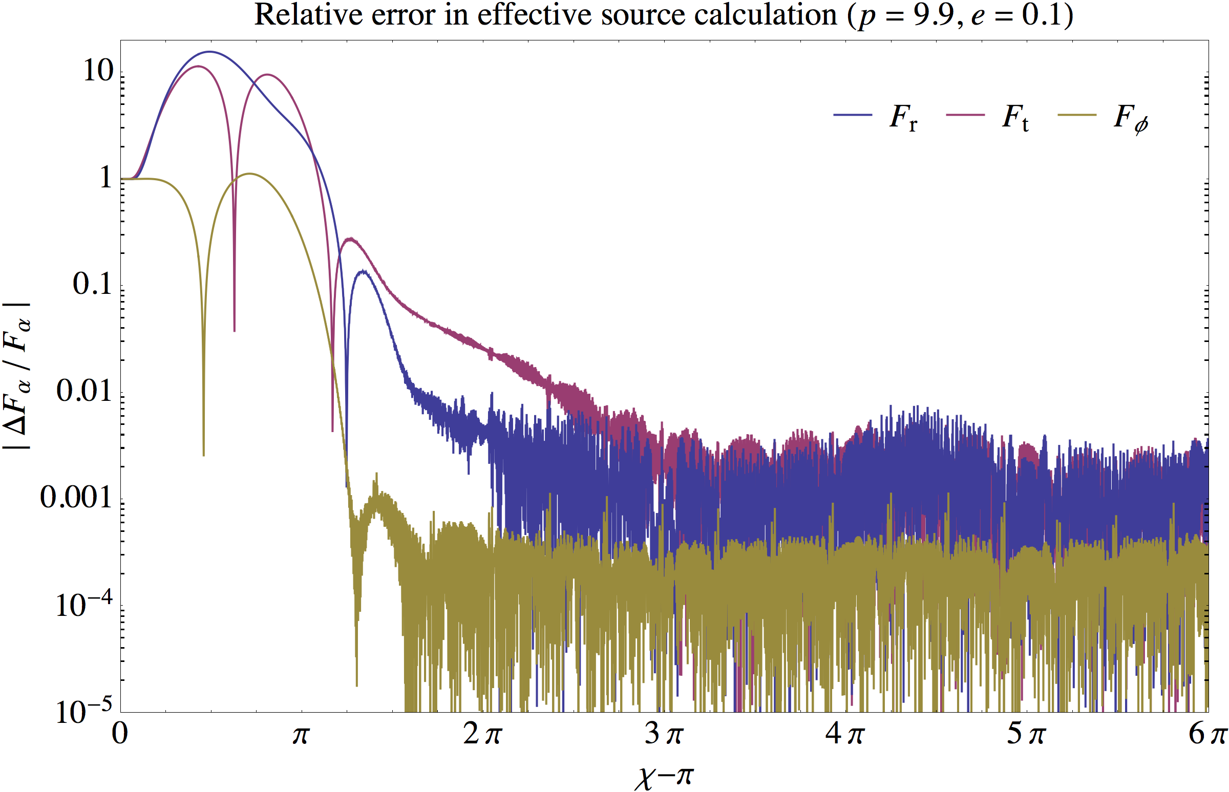


We see that the initial burst of junk radiation (coming from inconsistent initial data) contaminates the self-force for up to one orbit. After the junk radiation has radiated away, the self-force settles down to within of the reference value. The high-frequency oscillations in the error reflect the fact that the low-order differentiability of the solution on the world line introduces a finite differencing error which oscillates at the frequency with which the world line moves from one grid point to the next. This could be improved by using a higher order approximation to the singular field, thereby increasing the smoothness of the solution. This benefit would, however, come at the cost of a substantially more complicated (and computationally costly) effective source.
IV.2.2 Convergence
Our evolution code has been shown to converge cleanly at the expected order when evolving smooth initial data [47]. The convergence order is determined both by the order of finite differencing in the interior region and at the inter-patch boundaries. For example, for the 8-4 summation by parts operators used here, fifth order global convergence is to be expected.
However, our choice of approximation to the singular field yields an effective source which is only on the world line of the particle, and the evolved residual field is therefore at the same point. Elsewhere, the solution is expected to be perfectly smooth. Unsurprisingly, this lack of smoothness spoils any hope of clean high-order convergence of the solution. It was shown in Appendix A of [9] that for the wave equation in 1+1D, the errors are instead expected to converge at second order in the L2-norm for a source. It is also shown that the error is of high frequency with the frequency increasing with resolution. Thus, we cannot demonstrate pointwise convergence for the evolved fields; instead we expect that the amplitude of any noise generated near the world line will converge away at second order.

Figures 5, 6 and 7 show the convergence in , and for the , case by measuring errors relative to reference values from the (1+1) time-domain code. At the medium and high resolutions, the error is dominated by the high-frequency errors coming from the low differentiability of the solution near the world line and we see that the amplitude of the error converges away at approximately second order, as expected.
In contrast, we found that our lowest resolution runs also contained smooth finite differencing errors which scaled as the fifth power of the change in resolution. This error arises simply because of insufficient resolution in the angular directions (recall that our use of a window function in the polar direction introduces significant angular structure). The increase in resolution to angular cells was sufficient to decrease this error to below the level of the error arising from the nonsmoothness on the world line.


V Conclusion
In this paper, we reported the successful extension of the effective source approach to the case of eccentric orbits in the Schwarzschild geometry. This advance relied on many code adjustments, but principally on the construction of a generic effective source as detailed in [10]. Our code is now capable of calculating the self-force to within of of the reference value for the - and -components, and to within for the -component. We have also shown that at sufficiently high resolution our code is second-order convergent in the calculation of the self-force. This new code has been the basis of the first self-consistent simulation of a self-forced orbit for a scalar charge [8]. Finally, we have presented our self-force results in the form of “loops”, which give the self-force components through one radial cycle of an eccentric orbit. This manner of presenting eccentric-orbit self-force data makes some features apparent that are obscured when the data is presented as standard time series.
In principle, the effective source method can also be adapted to handle a generic orbit in the Kerr spacetime. The only essential challenge is the considerable additional complexity introduced in the calculation of the effective source. We see this as the natural next step in this developing research programme, for which results should be forthcoming.
Acknowledgements.
The authors thank Niels Warburton, Norichika Sago, Eric Poisson, Steven Detweiler, and Frank Löffler for helpful comments and many fruitful discussions that helped shape this work. I. V. acknowledges partial financial support from the European Research Council under the European UnionÕs Seventh Framework Programme (FP7/2007-2013)/ERC Grant No. 306425 “Challenging General Relativity” and from the Marie Curie Career Integration Grant LIMITSOFGR-2011-TPS, and would like to thank the hospitality of Jose Perico Esguerra and the National Institute of Physics, University of the Philippines-Diliman, where parts of this manuscript were written. B.W. gratefully acknowledges support from Science Foundation Ireland under Grant No. 10/RFP/PHY2847. Portions of this research were conducted with high performance computational resources provided by the Louisiana Optical Network Initiative (http://www.loni.org/) and also used the Extreme Science and Engineering Discovery Environment, which is supported by National Science Foundation Grant No. OCI-1053575 (allocation TG-MCA02N014). The authors additionally wish to acknowledge the SFI/HEA Irish Centre for High-End Computing (ICHEC) for the provision of computational facilities and support (project ndast005b). Some computations were also performed on the Datura cluster at the Albert Einstein Institute.*
Appendix A Flux formulas
In [9], the expressions for the energy flux through the event horizon and a large spatial 2-sphere were derived. This appendix similarly derives the corresponding expressions for the angular momentum flux at the horizon () in Kerr-Schild coordinates and at future null infinity () in Cartesian hyperboloidal coordinates.
Kerr-Schild and Schwarzschild coordinates are related according to
| (37) |
where is Schwarzschild time, is Kerr-Schild time, and in Kerr-Schild coordinates .
To implement hyperboloidal slicing (in the exterior region where the effective source vanishes, including ), we use the additional transformation :
| (38) |
| (39) |
where the choices for and in a neighborhood of are the same as in [34, 32] (following the notation of [34]):
| (40) |
| (41) |
so that is located at . In this coordinate system, the metric is singular at , so we finally apply a conformal transformation, . At , the conformal metric is regular.
The angular momentum fluxes through and are respectively given by
| (42) | ||||
| (43) |
where
| (44) |
is the stress-energy in the conformally-related space, is the rotational Killing vector, while and are the null generators of and , respectively.
Our goal is to write these flux formulas explicitly in terms of the quantities we compute in our code: the scalar field, , and its derivatives in Kerr-Schild and hyperboloidal coordinates.
We shall deal with the angular momentum flux through first. In Kerr-Schild coordinates, the Schwarzschild metric and its inverse are simply
| (45) | ||||
| (46) |
| (47) |
where again , , and .
The event horizon is essentially a surface of constant retarded time . In Kerr-Schild coordinates these surfaces of constant are
| (48) |
where is just a constant. In Kerr-Schild coordinates, the null generator of is then just
| (49) |
and the rotational Killing vector is
| (50) |
Putting everything together, we get
| (51) |
The angular momentum flux through the event horizon is then simply just
| (52) |
Now we turn to the flux through . The conformal metric close to can be shown to be
| (53) |
where we have used and , which follow from Eqs. (40) and (41).
The null generator of is then
| (54) |
We can also switch to Cartesian hyperboloidal coordinates, , defined by
| (55) | ||||
| (56) | ||||
| (57) |
so that the rotational Killing vector becomes
| (58) |
We then find that
| (59) |
which looks very similar to Eq. (51), except that all the quantities here pertain to the conformally-related space, and not the physical space.
Finally we get
| (60) |
For completeness, we also include here an explicit expression for the energy flux through . In [9], only the energy flux at spatial infinity was derived and was taken to be the limit of the flux through a spatial 2-sphere as the radius of the sphere approached infinity. With hyperboloidal slicing, the energy flux through is just
| (61) |
where is just the timelike Killing vector of the Schwarzschild spacetime. In hyperboloidal coordinates, the timelike Killing vector also has components given by
| (62) |
This then easily leads to the expression
| (63) |
References
- [1] B. Sathyaprakash and B. Schutz, Living Rev.Rel. 12, 2 (2009), arXiv:0903.0338 [gr-qc] .
- [2] P. Amaro-Seoane, B. Schutz, and C. F. Sopuerta, (2010), arXiv:1009.1402 [astro-ph.CO] .
- [3] P. Amaro-Seoane, S. Aoudia, S. Babak, P. Binetruy, E. Berti, et al., GW Notes 6 (2013), arXiv:1201.3621 [astro-ph.CO] .
- [4] M. Davis, R. Ruffini, W. Press, and R. Price, Phys. Rev. Lett. 27, 1466 (1971).
- [5] S. Detweiler, Astrophys. J. 225, 687 (1978).
- [6] L. Barack and D. A. Golbourn, Phys.Rev. D76, 044020 (2007), arXiv:0705.3620 [gr-qc] .
- [7] I. Vega and S. L. Detweiler, Phys.Rev. D77, 084008 (2008), arXiv:0712.4405 [gr-qc] .
- [8] P. Diener, I. Vega, B. Wardell, and S. Detweiler, Phys.Rev.Lett. 108, 191102 (2012), arXiv:1112.4821 [gr-qc] .
- [9] I. Vega, P. Diener, W. Tichy, and S. L. Detweiler, Phys.Rev. D80, 084021 (2009), arXiv:0908.2138 [gr-qc] .
- [10] B. Wardell, I. Vega, J. Thornburg, and P. Diener, Phys.Rev. D85, 104044 (2012), arXiv:1112.6355 [gr-qc] .
- [11] R. Haas, Phys.Rev. D75, 124011 (2007), arXiv:0704.0797 [gr-qc] .
- [12] C. W. Misner, K. Thorne, and J. Wheeler, Gravitation (Freeman, San Francisco, 1974).
- [13] C. Cutler, D. Kennefick, and E. Poisson, Phys.Rev. D50, 3816 (1994).
- [14] A. Pound and E. Poisson, Phys.Rev. D77, 044013 (2008), arXiv:0708.3033 [gr-qc] .
- [15] L. Barack and N. Sago, Phys.Rev. D81, 084021 (2010), arXiv:1002.2386 [gr-qc] .
- [16] T. C. Quinn, Phys.Rev. D62, 064029 (2000), arXiv:gr-qc/0005030 [gr-qc] .
- [17] R. Haas, (2011), arXiv:1112.3707 [gr-qc] .
- [18] P. Canizares and C. F. Sopuerta, Phys.Rev. D79, 084020 (2009), arXiv:0903.0505 [gr-qc] .
- [19] P. Canizares, C. F. Sopuerta, and J. L. Jaramillo, Phys.Rev. D82, 044023 (2010), arXiv:1006.3201 [gr-qc] .
- [20] P. Canizares and C. F. Sopuerta, Class.Quant.Grav. 28, 134011 (2011), arXiv:1101.2526 [gr-qc] .
- [21] N. Warburton and L. Barack, Phys.Rev. D81, 084039 (2010), arXiv:1003.1860 [gr-qc] .
- [22] N. Warburton and L. Barack, Phys.Rev. D83, 124038 (2011), arXiv:1103.0287 [gr-qc] .
- [23] P. Zimmerman, I. Vega, E. Poisson, and R. Haas, Phys.Rev. D87, 041501(R) (2013), arXiv:1211.3889 [gr-qc] .
- [24] N. Warburton, S. Akcay, L. Barack, J. R. Gair, and N. Sago, Phys.Rev. D85, 061501 (2012), arXiv:1111.6908 [gr-qc] .
- [25] S. A. Hughes, S. Drasco, E. E. Flanagan, and J. Franklin, Phys.Rev.Lett. 94, 221101 (2005), arXiv:gr-qc/0504015 [gr-qc] .
- [26] S. Drasco, E. E. Flanagan, and S. A. Hughes, Class.Quant.Grav. 22, S801 (2005), arXiv:gr-qc/0505075 [gr-qc] .
- [27] A. Pound, E. Poisson, and B. G. Nickel, Phys.Rev. D72, 124001 (2005), arXiv:gr-qc/0509122 [gr-qc] .
- [28] T. Hinderer and E. E. Flanagan, Phys.Rev. D78, 064028 (2008), arXiv:0805.3337 [gr-qc] .
- [29] Y. Mino, Phys.Rev. D67, 084027 (2003), arXiv:gr-qc/0302075 [gr-qc] .
- [30] L. Barack, Class.Quant.Grav. 26, 213001 (2009), arXiv:0908.1664 [gr-qc] .
- [31] M. J. Pfenning and E. Poisson, Phys.Rev. D65, 084001 (2002), arXiv:gr-qc/0012057 [gr-qc] .
- [32] I. Vega, B. Wardell, and P. Diener, Class.Quant.Grav. 28, 134010 (2011), arXiv:1101.2925 [gr-qc] .
- [33] A. Zenginoglu, Class.Quant.Grav. 25, 145002 (2008), arXiv:0712.4333 [gr-qc] .
- [34] A. Zenginoglu and M. Tiglio, Phys.Rev. D80, 024044 (2009), arXiv:0906.3342 [gr-qc] .
- [35] S. L. Detweiler and B. F. Whiting, Phys.Rev. D67, 024025 (2003), arXiv:gr-qc/0202086 [gr-qc] .
- [36] S. R. Dolan and L. Barack, Phys.Rev. D83, 024019 (2011), arXiv:1010.5255 [gr-qc] .
- [37] S. R. Dolan, L. Barack, and B. Wardell, Phys.Rev. D84, 084001 (2011), arXiv:1107.0012 [gr-qc] .
- [38] S. L. Detweiler, E. Messaritaki, and B. F. Whiting, Phys.Rev. D67, 104016 (2003), arXiv:gr-qc/0205079 [gr-qc] .
- [39] R. Haas and E. Poisson, Phys.Rev. D74, 044009 (2006), arXiv:gr-qc/0605077 [gr-qc] .
- [40] E. Poisson, A. Pound, and I. Vega, Living Rev.Rel. 14, 7 (2011), arXiv:1102.0529 [gr-qc] .
- [41] F. Loffler, J. Faber, E. Bentivegna, T. Bode, P. Diener, et al., Class.Quant.Grav. 29, 115001 (2012), arXiv:1111.3344 [gr-qc] .
- [42] T. Goodale, G. Allen, G. Lanfermann, J. Massó, T. Radke, E. Seidel, and J. Shalf, in Vector and Parallel Processing – VECPAR’2002, 5th International Conference, Lecture Notes in Computer Science, Vol. 2565 (Springer, Berlin, 2003).
- [43] Cactus developers, “Cactus Computational Toolkit,” http://www.cactuscode.org/.
- [44] E. Schnetter, S. H. Hawley, and I. Hawke, Class.Quant.Grav. 21, 1465 (2004), arXiv:gr-qc/0310042 [gr-qc] .
- [45] E. Schnetter, Carpet: Adaptive Mesh Refinement for the Cactus Framework.
- [46] E. Schnetter, P. Diener, E. N. Dorband, and M. Tiglio, Class.Quant.Grav. 23, S553 (2006), arXiv:gr-qc/0602104 [gr-qc] .
- [47] P. Diener, E. N. Dorband, E. Schnetter, and M. Tiglio, J.Sci.Comput. 32, 109 (2007), arXiv:gr-qc/0512001 [gr-qc] .
- [48] E. N. Dorband, E. Berti, P. Diener, E. Schnetter, and M. Tiglio, Phys.Rev. D74, 084028 (2006), arXiv:gr-qc/0608091 [gr-qc] .