Characteristic times of biased random walks on complex networks
Abstract
We consider degree-biased random walkers whose probability to move from a node to one of its neighbors of degree is proportional to , where is a tuning parameter. We study both numerically and analytically three types of characteristic times, namely: i) the time the walker needs to come back to the starting node, ii) the time it takes to visit a given node for the first time, and iii) the time it takes to visit all the nodes of the network. We consider a large data set of real-world networks and we show that the value of which minimizes the three characteristic times is different from the value analytically found for uncorrelated networks in the mean-field approximation. In addition to this, we found that assortative networks have preferentially a value of in the range , while disassortative networks have in the range . We derive an analytical relation between the degree correlation exponent and the optimal bias value , which works well for real-world assortative networks. When only local information is available, degree-biased random walks can guarantee smaller characteristic times than the classical unbiased random walks, by means of an appropriate tuning of the motion bias.
pacs
89.75.Hc, 05.40.Fb, 89.75.KdIn the last decade or so the quantitative analysis of networks having different origin and function, including social networks, the human brain, the Internet, the World Wide Web, has revealed that all these systems exhibit comparable structural properties at different scales, and are more similar to each other than expected [1, 2]. It has been found that the structural complexity of networks from the real world usually has a significant impact on the dynamical processes occurring over them, including opinion dynamics [3], epidemics [4] and synchronization [5].
Random walks are the simplest way to explore a network, and are one of the most widely studied class of processes on complex networks [6, 7]. Different kinds of random walks have been used to implement efficient local search strategies [8, 9], and also to reveal the presence of hierarchies and network communities [10, 11]. Particular attention has been devoted to the study of the characteristic times associated to random walks, such as the mean return times, or the mean first passage times, respectively the average time the walker takes to come back to the starting node or to hit a given node [12]. Such characteristic times can be determined analytically for random walks on regular lattices [13], but their calculation for graphs with heterogeneous structures is still the object of active research [14, 15]. Recent results include the derivation of analytic expressions for the characteristic times of unbiased random walks on Erdös–Rényi random graphs [16], on fractal networks [17, 18, 19, 20] and on particular classes of scale-free graphs [21]. To date, only approximate solutions are available for random walks on real networks [22, 23, 24, 25].
A class of random walks which is particularly interesting to consider on heterogeneous networks is that of degree-biased random walks. In a degree-biased random walk, the probability to move from a given node to one of its neighbors, of degree , is proportional to , where is a tuning parameter. According to the sign of the bias parameter , the walkers preferentially move either towards hubs or towards poorly connected nodes [26]. Biased random walks have been recently employed for community detection [27] and to define new centrality measures [28, 29]. Furthermore, analytical results on the characteristic times of degree-biased random walks have been obtained for specific classes of random graphs in the mean-field approximation [30]. However, the structure of real networks is far from being random, and several empirical evidences suggest that the presence of degree-degree correlations can affect the dynamics of the walk [31]. For instance, the authors of Ref. [26] have shown that the value of entropy rate of biased random walks on real correlated networks substantially deviates from the prediction for the corresponding randomized graphs. Similarly, more recent works show that degree-biased random walks can approximate maximally entropic walks, but the quality of such approximation depends again on degree-degree correlations [32, 33].
In this Article we study, both numerically and analytically, three types of characteristic times for biased random walks, namely mean return times (MRT), mean first passage times (MFPT), and mean coverage times (MCT). We consider different synthetic graphs and a large data set of social, biological and technological complex networks from the real world, and we study the effect of the bias parameter on the characteristic times of the walk, focusing on the values that guarantee minimal return, first passage and coverage times. Our main result is that the characteristic times of biased random walks on real-world networks sensibly deviate from those observed in uncorrelated graphs. In particular, we prove analytically that the minimum MRT in Erdös–Rényi and scale-free random graphs is always obtained for , while we show through numerical simulations that the minimum MRT in real-world networks is obtained for values of that significantly deviate from . We find that the value depends on the presence and sign of degree-degree correlations in the network, and in particular that for assortative networks , while for disassortative networks . We show that in the case of networks in which the expected degree of the first neighbors of a node with degree is a power law, i.e. when as observed in many real-world networks, it is possible to derive an approximate relation between the optimal bias value and the exponent . This approximation works well for assortative networks in which, for any given value of , the predicted optimal value of is close to the real optimum. We also analyze the MRT for nodes of a given degree class , and we derive a closed form, valid for uncorrelated scale-free graphs, to calculate the value of the bias which minimizes the MRT for nodes of degree . We also discuss the results found for MFPT and MCT, which suggest that the optimal value of for MRT on a given network is a quite accurate approximation for the values of which optimize the MFPT and the MCT on the same network.
The paper is organized as follows. In Section I we introduce degree-biased random walks and we provide the definitions of return, first passage and coverage times. In Section II we study how the MRT depends on the value of the bias parameter , and we compare the analytical predictions of characteristic times, which assume the absence of degree correlations, with the numerical results obtained on a large data set of real-world networks. We also investigate the dependence of the MRT on the degree of the starting node. In Section III and Section IV we study, respectively, the behavior of MFPT and MCT on real-world networks, and we show that the relation between the sign of degree-degree correlations in a graph and the dynamics of the walkers on the graph are indeed similar to those found for MRT. In Section V we provide a more detailed discussion of the results presented in the paper, we derive an analytical relation between and , and we indicate possible applications to several problems connected with characteristic times of biased random walks. Finally, in Section VI we draw some conclusions and we suggest possible future directions of research in this field.
I Degree-Biased Random Walks
Let us consider an undirected and unweighted graph with nodes and edges. Denote as the adjacency matrix of graph , i.e. the symmetric matrix whose entry is equal to if an edge exists between node and , and is otherwise. We consider the following dynamical process occurring on the graph: a walker that at each time step moves from a node to one of its neighbors with a probability proportional to the -power of the degree of the target node. The process corresponds to a discrete-time Markov chain [34] on the state space defined by the transition matrix , whose each entry is equal to the probability for a walker on node to jump to one of its neighbors , and reads:
| (1) |
The exponent is the control parameter that allows to tune the dependence of the process on the node degree. When the random motion is biased towards high-degree nodes (hubs), while when the walkers move with higher probability to neighbors with low degree. When the common (unbiased) random walk is recovered. The fundamental quantity to describe a random walk is the occupation probability distribution . Being the probability that a walker is at node at time , then the probability of being at node at time is given by:
| (2) |
or in vector notation: . A fixed point solution of the latter equation, such that , is called stationary distribution. If the transition matrix is primitive, i.e. if the graph is connected and contains at least one odd cycle, the Perron-Frobenius theorem guarantees that always exists, is unique, and
i.e. all initial occupation probability distributions converge to the stationary distribution [35]. In particular, the stationary distribution associated to the transition matrix (1) of a degree-biased random walk is [26]:
| (3) |
When , Eq. (3) reduces to:
| (4) |
which states that for unbiased random walks the number of walkers at a node is proportional to the degree , so that the dynamic process is completely characterized by the degree sequence of the graph. Conversely, when , the stationary distribution does not depend only on the degree but also on the degrees of the first neighbors of node , through the coefficient . The stationary probability distribution is therefore sensitive to the degree sequence and also to the presence of degree-degree correlations in the network. It is interesting to notice that the majority of real-world networks exhibit degree-degree correlations, meaning that their nodes are found to be preferentially connected with other nodes having either similar or dissimilar degree [36, 37, 38]. Consequently, in these networks the stationary probability distribution can sensibly deviate from that observed on a random graph having the same degree distribution and no degree-degree correlations. Degree-degree correlations are fully described by the joint probability , that represents the likelihood that nodes with degree and are connected through an edge, or equivalently by the conditional probability distribution , which represents the probability that a node of a given degree is connected to a node of degree . The type of correlations is usually characterized by the average degree of the nearest neighbors of nodes with degree . This can be written in terms of the conditional probability distribution as [36]:
Networks are called assortative when is an increasing function of and disassortative when is a decreasing function of [36]. In many real-world networks the nearest neighbors average degree is found to be a power-law function of , i.e. , so that the exponent —often called degree correlation exponent— can be used to quantitatively characterize degree correlations. A positive exponent indicates assortative correlation while a negative value indicates disassortative ones.
In this paper we are interested in the typical times of degree-biased random walks. In particular, assuming that a walker is at node at time and moves according to Eq. (1), we consider the expected time that the random walker needs to:
- •
come back to node for the first time, referred to as Mean Return Time (MRT) and denoted as ,
- •
reach a node () for the first time, referred to as Mean First Passage Time (MFPT) and denoted as ,
- •
visit all nodes in the network at least once, referred to as Mean Coverage Time (MCT) and denoted as .
In the following sections we explore how the three characteristic times defined above are affected by the bias in the random walk. In particular we will focus on the value of the bias parameter which respectively minimizes MRT, MFPT and MCT. We use a data set consisting of many assortative and disassortative medium-to-large sized real-world networks, and we will show how degree biased random walks can highlight assortativity or disassortativity from a dynamical point of view.
II Mean Return Time
It is possible to prove that the mean return time of a random walk on a graph is equivalent to the inverse of the stationary distribution of the walk [39]:
| (5) |
In order to summarize in a single value the typical return time for the entire network, we define the graph mean return time as the average of over all nodes:
| (6) |
Empirical evidences. — In the case of a degree-biased random walk, depends on because the stationary distribution depends on as in Eq. (3). In Fig. 1 we show the graph mean return time as a function of for three networks, namely a scale-free network with nodes, with and average degree , constructed by the configuration model [40], the scientific collaboration network of scientists in condensed matter (SCN) [41], having nodes and edges, and a sample of the Internet at the Autonomous System level (InternetAS) [36], having and edges. The values of are rescaled by the network size .
The networks reported in Fig. 1 are representative of the general behavior observed in the entire data set. In fact, for all the considered networks is always a convex function of , with a single minimum, denoted by , observed at a value of denoted as . For the uncorrelated scale-free network we find and . The same result has been found for Erdös–Rényi random graphs and for other uncorrelated scale-free networks constructed through linear preferential attachment [42]. As shown in Table 1, as the average degree of a synthetic network increases, the corresponding value of approaches . Also the minimum return time becomes progressively more similar to the size of the network: . These results are in agreement with what has been found in Ref. [30]. We will give an analytical explanation of the fact that for uncorrelated networks at the end of this Section.
From Fig. 1 it is clear that the dynamical behavior of biased random walks on real-world networks considerably deviates from that observed in uncorrelated synthetic networks. In fact, if a network has degree-degree correlations then the minimum of always occurs for values of larger than . In particular, for SCN we have while for InternetAS we have (refer to Table 1 for the values of in each of the real-world networks considered in this study). As we see in the Figure, the value of in real-world networks is also highly sensitive to the value of , and can be considerably lower than the value of MRT corresponding to an unbiased random walk () on the same network. For instance, in SCN the value of is about half the value of corresponding to an unbiased random walk. This result indicates that a carefully chosen value of the bias parameter can significantly reduce the characteristic times of degree-biased random walks.
In Fig. 2 we report the values of and for each network in the data set. For those networks with the minimum value is only slightly greater than the size of the network , while the differences are more pronounced in the region . Notice that all the networks with clear assortative degree-degree correlations (reported in green) have a value of , while disassortative networks (reported in red) have . This result indicates that the presence of degree-degree correlations has a significant impact in the values of , and consequently on the performance of a biased random walk on a graph in terms of exploration speed.
The relation between the degree-correlation exponent and the value of is shown in Fig. 3. The values corresponding to real-world networks lie almost exclusively in the top-left and in the bottom-right quadrants, respectively corresponding to and . Fig. 3 shows very clearly that the value of is always in the interval for assortative networks and larger than for disassortative ones.
To further investigate the special role played by the bias parameter we have considered a large set of synthetic networks, in which we tuned the level and sign of degree-degree correlations through the edge-swapping procedure described in Ref. [43]. This procedure, discussed in details in Appendix, starts from an uncorrelated network and artificially introduces a prescribed amount of either assortative or disassortative degree-degree correlations by rewiring the edges of the graph without modifying the degree sequence. As a result, this algorithm allows to investigate the relation between the value of and of a network by varying continuously the correlation exponent while preserving the degree sequence.
The black curve in Fig. 3 has been obtained by starting with a configuration model scale-free network with nodes, and [44], and by running the swapping procedure to introduce assortative or disassortative correlations. We notice that by performing assortative swaps the value of increases considerably, while remains asymptotically confined below . Conversely, few disassortative swaps are enough to determine a fast change on , which enters the region where the majority of real-world disassortative networks lie.
In Fig. 4 we report as a solid line the values of as a function of the degree-correlation exponent for the same set of synthetic networks considered in Fig. 3. Filled squares represent the values obtained on real-world networks. We observe that is considerably larger than for disassortative networks, while it is closer to for assortative networks. Notice that the MRT of the synthetic network with tunable degree correlations (solid black line) is consistently smaller than that of any real-world network, with the only exception of the C.Elegans neural network.
Analytical arguments. — The numerical analysis of MRT suggests that, for uncorrelated networks, , so that the deviations from this value observed in real-world networks should be due to the presence of degree-degree correlations. Here, we provide an analytical proof of the fact that for uncorrelated graphs in the mean-field approximation, and we compare this analytical prediction with numerical results on real-world networks. In the mean-field approximation a graph is described by the annealed adjacency matrix:
| (7) |
where the value represents the probability to find an edge connecting node and node , having degrees and , if the nodes are connected uniformly at random. In fact, let us imagine a network where each node has stubs to be paired with some of the stubs of other nodes. If is the total number of links there are of such free stubs. Among these stubs, only are incident on node . Therefore, there are ways a stub of node can be connected with node over a total of possible pairings with other nodes. One obtains the expression for in Eq. (7) by observing that node has different stubs to connect with one of the stubs of . If we plug Eq. (7) into Eq. (3) we obtain:
| (8) |
which gives
| (9) |
and
| (10) |
in agreement with the result found in Ref. [30].
It is straightforward to verify that when . Moreover, one can easily verify that for Erdös–Rényi graphs the minimum value of is obtained for . In order to see this fact, we replace the average over nodes in Eq. (10) with an integral over degree classes . We denote with the degree distribution of Erdös–Rényi graphs (this distribution is binomial, and can be approximated by a Poisson distribution for large ). Differentiating with respect to to find the minimum value of we have:
The latter expression is equal to 0 when , since we have and the last two terms are equal and opposite in sign. Analogously we can derive the minimum value of also for uncorrelated networks with power-law degree distribution :
| (11) |
where the integrability conditions are satisfied if is in the range , and which is compatible with the values of observed in real-world networks.
Differentiating Eq. (11) with respect to we get again the value , while the second derivative is always positive, as expected. It is worth noticing that the result is independent from the value of the scaling exponent of the degree distribution and from the maximum degree in the network, .
The quantity is an average over all graph nodes. However, Eq. (9) allows also to compute the value that minimizes the return time for nodes having a certain degree . In the case of Erdös–Rényi graphs a large number of nodes have the same degree because the degree distribution is picked around and, as a result, the values of return times are very similar for most of the nodes. For real-world networks, instead, the degree distribution is often heterogeneous and the the return time sensibly depends on the degree of the starting node. Differentiating Eq. (9) with respect to we get:
| (12) |
being .
Replacing the average over nodes with the integral over degree classes, and considering networks with power-law degree distributions and with minimum and maximum degree and we get
| (13) |
Integrating Eq. (13) and plugging in Eq. (12) we obtain:
| (14) |
where . The return time for nodes of a given degree class takes its minimum at the value of which satisfies the previous equation. Excluding the indeterminate case , Eq. (14) has only one solution for each value of .
In the three top panels of Fig. 5 we report the return time as a function of for different degree classes (solid lines), compared with the average return time of the same graph (black dotted lines). The three panels correspond, respectively, to (a) a configuration model scale-free graph with , (b) InternetAS and (c) SCN. These plots show that a wrong choice of the biased parameter can result in a large increase of the return time. For instance in Fig. 5 (c) the minimum return time for the degree class occurs for and is about four times smaller than the return time obtained at (refer to the vertical dashed lines for guidance).
In the three bottom panels of Fig. 5 we report, as a function of , the value which optimized the MRT for nodes having degree . The black crosses are the numerical results, while the solid blue line is the prediction in mean-field obtained from the zeros of Eq. (14). We notice an excellent agreement between the numerical results and the mean-field solution in the case of the uncorrelated scale-free graph (panel (d)), while for real-world networks (panel (e) and (f)) we observe considerable deviations from the analytical prediction, evidently due to the presence of degree-degree correlations. From the point of view of network exploration, Eq. (14) turns out to be useful when an agent is sent through the network in order to collect information and then has to come back to its starting point [45]. In fact, this equation gives insight about how to fine-tune the bias parameter in order to increase or decrease the time required (on average) by the agents to come back to the starting nodes with the collected information. It is worth noticing that small changes in can produce large variations in the return times, thus highlighting the importance of a proper tuning of the motion bias.
III Mean First Passage Time
In this Section we focus on the mean first passage time, showing that the interplay between degree correlations and the dynamics of biased random walks produces qualitatively similar results to those found for the mean return time.
We denote as the expected time needed for a random walker to reach node for the first time when starting from node . If the transition matrix of the walker is primitive, it is possible to determine by using the fundamental matrix of the Markov chain associated to the random walk [39]. The fundamental matrix is defined as:
| (15) |
where each row of is equal to the stationary probability distribution and is the identity matrix. The mean first passage time is then equal to:
| (16) |
where and are the entries of the fundamental matrix . Notice that in general . We define the graph mean first passage time as the average of the first passage time over all possible node pairs:
| (17) |
Notice that in general the calculation of the fundamental matrix in Eq. (15) is computationally intensive, since it requires the inversion of a matrix, and is practically unfeasible for large networks. For this reason we used the fundamental matrix only to compute the mean first passage time for relatively small networks (), while we resorted to agent-based simulation for larger networks (see Appendix for a description of the employed agent-based algorithm).
As found for the global mean return time , also is a convex function of the bias parameter with a single minimum at . This is illustrated in Fig. 6. Again, the position of the minimum is at only for uncorrelated networks (see Table 1). We also notice that for disassortative real-world networks as already found in the case of the mean return time. Conversely, some assortative networks can have a value which is not in the range . It is worth noticing that the minimum value in real-world networks is significantly smaller than the MFPT for unbiased () random walks, or for the case of uncorrelated networks (). In Fig. 6 we plot, for all the networks in the data set, the minimum value of the graph first passage time rescaled by the number of nodes . Despite there is no clear separation at between assortative and disassortative networks, as observed for the MRT, the behavior is similar to that shown in Fig. 2: the farther gets from , the more deviates from .
A comparison between the values of for MFPT and MRT is shown in Fig. 6. Excluding the network of the US power grid (indicated in the figure as USPower), the value of the Pearson’s linear correlation coefficient between and is . Despite the two values of are not equal for all networks, the strong positive correlation we observe is quite remarkable. We notice that the US power grid is the only spatially embedded network in the data set, so that its exceptional values of can be due to spatial constraints, which are absent in the other networks studied. The existence of a relatively strong positive correlation between and could have interesting practical applications. In fact, in order to obtain a walk having a small graph MFPT on a large network, it is possible to use as an approximation of , so that one can obtain a quasi-optimal biased random walk with respect to MFPT without the need to invert the fundamental matrix of the graph, which is practically impossible for large networks.
IV Mean coverage time
The last characteristic time under investigation is the mean coverage time (MCT) , defined as the expected number of time steps required for the walker to visit all the nodes of the graph at least once when starting from node . We also study the graph mean coverage time , defined as an average of over all the graph nodes:
| (18) |
We have computed the graph mean coverage time for all but two networks in the data set by means of an agent-based simulation and by averaging over many realizations of the walk as described in the Appendix. The asymptotic lower bound on the coverage time for the unbiased () random walk on a generic graph is given by [46]:
| (19) |
where the equality is satisfied for the complete graph of nodes, i.e. the graph in which there is a link between every pair of nodes. The inequality (19) implies the following lower bound for the global mean coverage time:
| (20) |
We therefore normalize the obtained values of by the quantity .
In Fig. 7 we report such normalized quantity as a function of the bias parameter for a configuration model scale-free network, SCN and InternetAS. The mean coverage time is a convex function of with a single minimum at . As for MRT and MFPT we notice that the minimum of the global mean coverage time for the uncorrelated scale-free graph occurs at , and that the minimum value is very close to the lower bound given by Eq. (20). Real-world networks have instead values of significantly higher than the lower bound.
We notice that the MCT is more sensitive to than MRT and MFPT (the typical concavity of MCT in Fig. 7 is narrower than the ones observed for MRT and MFPT, respectively in Fig. 1 and in Fig. 6). For instance, in SCN the minimum mean coverage time, , is about times smaller than the mean coverage time obtained for or for on the same graph, which is . Instead, disassortative networks like InternetAS have a minimum value of the coverage time that is similar to that for the unbiased case, while extremely different from the value at .
In Fig. 7 we report the values of and for all the networks in the considered data set. The results are qualitatively similar to those reported in Fig. 2 and Fig. 6. Although for a given network the minimum of occurs at , it is evident from Fig. 7 that the two values are positively correlated (the Pearson’s linear correlation coefficient is ).
We have investigated the differences between the optimal values of for the three characteristic times comparing , and for a set of synthetic networks generated through the swapping procedure (the starting network in this case is a configuration model with , and ). The results (figure not shown) suggest that synthetic assortative networks have equal optimal bias values (), so that the deviations from the bisector in Figures 6 and 7 might be due only to fluctuations in the pattern of degree correlations of real-world networks. Instead, in the case of synthetic disassortative networks we observe deviations from the bisector of the same order of those observed in real-world networks.
V Discussion
In this section we discuss in detail some of the results reported in the paper, we provide a mechanistic explanation of the variations of observed in real-world networks and we outline possible applications to practical problems.
Deviations from . — The results reported in Fig. 2 confirmed that the value of which minimizes the MRT in real-world networks sensibly deviates from the value predicted for uncorrelated graph, and that this deviation seems to depend on the sign and magnitude of degree-degree correlations. We notice that, in the absence of degree correlations, the stationary distribution of walkers is given by Eq. (8), which for corresponds to a uniform distribution of walkers across the nodes of the network, i.e. . Consequently, the minimum value of MRT for uncorrelated graphs is obtained for a uniform distribution of walkers and is equal to (see Eq. (10)). We argue that the minimum of MRT in a generic network is always obtained for a value of which induces the distribution of walker that is the closest possible to a uniform one.
We start by noticing that, according to Eq.(6), is the harmonic mean of the stationary distribution . By using Jensen’s inequality [47], it is possible to prove that any stationary distribution which is not uniform produces a value of the mean return time which is larger than (or at most equal to) that obtained from a uniform (which is equal to ):
| (21) |
where . We observe that if a graph is not uncorrelated, and especially if the graph has assortative degree correlations, then the stationary distribution of the biased random walk obtained for is generally far from being uniform, while the stationary distribution corresponding to is usually very close to a uniform one. And in fact, Fig. 2 confirms that for assortative networks the value of is very close to , despite larger deviations are observed for disassortative networks. Thus we assume that, for a given network, the discrepancy between the observed value of and the prediction for uncorrelated networks is indeed due to the necessity to obtain a stationary distribution as close as possible to a uniform one.
If this hypothesis is correct, it should be possible to determine the value of by imposing that the resulting stationary occupation probability distribution is as close as possible to . Let us consider the case of assortative networks, and assume that the expected degree of the first neighbors of a node having degree is a power-law, i.e.:
| (22) |
where is a normalization constant. Let us also make the assumption that the fluctuations in the degree of the neighbors of a node with degree are negligible, so that if is a first neighbor of node we can write:
By plugging Eq. (22) in Eq. (3) we get:
| (23) |
Imposing that is a uniform distribution, i.e. that , we obtain that should satisfy the equation:
| (24) |
In Fig. 8 we show the curve (solid blue line) together with the values corresponding to real-world networks. Notice that for uncorrelated networks, i.e. when , we obtain the analytical prediction , while for maximally assortative networks, i.e. for , we get . Also, the values of for real-world assortative networks are close —but admittedly not identical— to the prediction of Eq. (24). The observed discrepancies between theory and observations are due to the fact that, despite in real-world networks we usually have , the fluctuations in the degree of the nearest neighbors of a node with degree are not negligible. Therefore, if is a neighbor of then , and consequently the second of the two assumptions used in the derivation of Eq. (23) and Eq. (24) does not hold.
The case of disassortative networks is a bit more cumbersome, due to the constraints introduced by a discrete degree sequence (namely, a node cannot have a degree smaller than or larger than ). In particular, it is possible to define:
| (25) |
obtaining an equation similar to Eq. (24). Unfortunately, such equation has a discontinuity at and does not match the values of observed in real-world disassortative networks.
In the absence of an analytical argument for disassortative networks, we computed numerically the value of which minimizes the variance of the stationary occupation probability distribution. In fact, provides a rough estimation of how far the distribution is from a uniform one (for which ). The results are reported in Fig. 9, in which we show, for each network in the considered data set, the value of which minimizes the MRT and the value which minimizes the variance of . Notice that for assortative networks we have a strong positive correlation between and , with . Conversely, for disassortative networks the two values are negatively correlated, and seem to be connected by the relation . These results confirm that there is indeed an intimate relation between the variance of the stationary state distribution of walkers obtained for a given value of the motion bias and the corresponding MRT, and suggest that the optimization of the mean return time is obtained for a value of which guarantees a stationary distribution as close as possible to a uniform one.
Applications. — The results shown in this paper can have interesting applications in several different contexts, from the control of diffusion processes to the successful advertisement of products and services on online social networks. A typical example is that of congestion control in communication and transport systems, such as the Internet, the WWW, P2P networks and road networks. In these systems traffic is usually modeled through simple packet generation and routing algorithms. At each time step, a certain number of new packets is introduced in the system, and each packet is assigned a source and a destination node. The nodes of the network route packets according to a certain policy (which might be a biased random walk), and have a fixed delivery capacity . When a packet arrives at its destination node, it is removed from the system. An interesting quantity that characterizes the emergence of congestion is the critical packet generation rate , defined as the number of new packets above which the number of packets removed from the system per unit time is smaller than the number of new packets per unit time introduced in the network. Under the condition the number of packets flowing in the network keeps increasing with time, leading to congestion. In Ref. [48] it has been shown that, for a routing strategy based on biased random walk, and the graph mean first passage time are related by the equations:
| (26) |
| (27) |
where is the delivering capacity. Eq. (26) shows that the value of depends on through both and . This implies that in order to maximize one has to minimize the product . By noticing that, in assortative networks, for we obtain a which is the closest possible to a uniform distribution (according to the results shown in Fig. 9) and, at the same time, we get an almost minimal value of (due to the strong positive correlation between and ), we can conclude that a good approximation for the value of the bias which maximizes can be obtained by setting . Unfortunately, this reasoning does not work in disassortative networks, for which the value of that minimizes does not coincide with the value of alpha which minimizes . In this case, the optimal critical packet rate depends on the trade-off between the homogeneity of the stationary occupation probability distribution and the corresponding value of . This is an example of how the correlation between the optimal values of and the sign and magnitude of degree-degree correlations can be used to avoid congestion and improve transport performance on a given network.
The results of this paper might also find application in the field of optimal network crawling, i.e. the exploration of the structure of a graph by means of agents performing random walks over it. Examples include the sampling of online social networks (e.g., Facebook and co-purchasing networks) and online communication networks (e.g., the World Wide Web and Twitter). In particular, exploring the network at the fastest possible speed corresponds to minimizing the MCT. As we have seen, this is achievable by using a degree-biased random walk with , since there is a pretty strong correlation between and . If the network is assortative, which is actually the case for the majority online social networks, the value of which optimizes the coverage time will lie in and can be obtained using Eq. (24) where the correlation exponent can be measured from a relatively small sample of the graph of interest. If instead the network is disassortative, as usually happens for online communication networks, then the value of should be chosen in the range and a good hint is provided by the value (see Fig. 9). Such value can be computed taking into account a small representative sample of the degree sequence of the graph. In both cases, an appropriate tuning of the bias parameter will outperform the standard unbiased random walk.
Another interesting application of the relationship between assortativity and optimal graph traversal could be that of information retrieval. In a recent work [49] it has been shown that the biased random walk on the directed network of Wikipedia pages can be used to implement an algorithm able to retrieve professional skills from an arbitrary text (e.g., a curriculum vitae). The authors have shown that the performance of the system can be optimized by means of an appropriate tuning of the motion bias . The results reported in Table 2 of Ref. [49] show that the best performance of the retrieval system are achieved for between and and in particular for which is a reasonable optimal value of the motion bias considering that the undirected version of the network of Wikipedia pages is known to be disassortative. Therefore, the generalization of the present study to the case of directed networks could provide theoretical insights and guidelines for the optimal choice of the bias parameter in skill retrieval system.
Finally, another possible application of these results concerns social-marketing campaigns. Today the advertising of products and services is more often conveyed through online social networking platforms. Customers are promised a reward if they promote a certain range of products to their on-line friends, and usually they get an equal reward for each friend that adopts the product/service. If we assume that the diffusion of the advertising can be regarded as a random motion, then promising equal rewards is not the best diffusion strategy, because customers will not have any reason to preferentially advertise the product to any of their neighbors in particular, and will therefore choose one of their friends at random, with equal probability. If we look to the advertisement as a walker which jumps from one customer to another, this strategy would correspond to an unbiased random walk(). Our results about mean coverage time suggest instead that the diffusion speed (i.e. the number of advertised users per unit time) can be increased if the customer is rewarded proportionally to a biased transition probability, i.e. if the customer receives a reward proportional to the power of the degree of the friend who has adopted the suggested product/service. The optimal bias parameter can be directly computed if the network topology is entirely known or, given that social networks are often assortative, it can be guessed using Eq. (24). This also disproves the intuitive idea that the best strategy is to always advertise the highly connected users.
VI Conclusions
Random walks are the simplest way to visit a network, and degree-biased random walks, which make use of information about the degree of destination nodes, are particularly suited to highlight the presence of degree-degree correlations. In this paper we have focused on the typical times of biased-random walks, namely on the expected time that a walker needs to come back to its starting node (MRT), to hit a given node (MFPT), or to visit all the nodes of the network (MCT). We have studied how such characteristic times depend on the value of the motion bias . We have proved analytically that, in the mean-field approximation, the value that minimizes the characteristic times in uncorrelated networks is equal to . This corresponds to a walk in which the probability to move to a node is inversely proportional to its degree. As shown by numerical simulations, the mean-field approximation works pretty well for uncorrelated networks. However, real-world networks are characterized by non-trivial degree-degree correlations and, as a result, the characteristic times of degree-biased random walks on real-world networks deviate from those obtained by using the mean-field approach, as we have shown in the paper by studying a large data set of medium to large real-world networks.
In particular, the value of sensibly differs from , in a way that depends on the sign of the degree-degree correlations. We have found that optimal values of the bias parameter lie between and for a large number of real-world networks. In addition to this, we have shown that the minimum characteristic times occur preferentially for in the range for assortative network, and for in the range for disassortative ones. We have derived an approximate analytical relation between and the degree-correlation exponent , which might be useful to refine the choice of the optimal bias for assortative networks, and we have shown numerically that the value of the mean return time obtained for a given value of is related with the heterogeneity of the corresponding stationary probability distribution of the walk.
By discussing several different possible applications of these results, we have stressed the fact that the minimization of characteristic times may be useful in many domains, from mitigation of network congestion to successful product advertisement in online social networks. In general, when only local information is available, degree-biased random walks can achieve better exploration performance than unbiased random walks, by appropriately tuning the bias parameter according to the global structural properties of the graph at hand.
Appendix
We describe here the algorithm we have used to generate graphs with tunable degree-degree correlations, and the agent-based approach used to estimate the mean coverage time and the mean first passage time in large graphs.
Swapping algorithm. In Fig. 3 and Fig. 4 we have reported the values of the degree-correlations exponent and the motion bias which minimizes the return time for a set of graphs with the same degree sequence of a chosen starting graph and tunable degree-degree correlations. An increasing amount of assortative or disassortative correlations is introduced by repeatedly applying the edge swapping procedure described in Ref.[43] to an initially uncorrelated graph. Each swap is performed as follows. Two edges connecting four different nodes are randomly selected and the nodes at the ends are ordered according to their degree . The two edges are then removed. Positive assortative correlations are introduced by connecting the two nodes with the smaller degrees and the two nodes with the larger degrees. Instead, disassortative correlations are introduced by connecting the node with the smallest degree with the node with the largest degree and the two remaining nodes with intermediate degrees. In order to preserve the degree sequence, all swaps that produce parallel edges are not allowed. Fig. 10 and Fig. 11 illustrate the two types of swaps.


Agent-based simulation for MFPT and MCT.
The MFPT and MCT
are estimated by means of an agent based simulation. In both cases we
simulated a walker which moves across the nodes of the network
according to the transition probability given in
Eq. (1).
The simplest way to compute the characteristic times is to wait until
the walker, started at a randomly selected node, explores all the
nodes at least once. At that point the value of is given by the
total number of time steps spent by the walker to visit all the nodes,
while can be obtained by storing in memory the first passage
times to all other nodes during the simulation. However, despite this
procedure is pretty simple to implement, it is not suitable to obtain
robust results in a reasonable amount of time. In fact, in order to
have an estimate of and , we need to average over a
sufficiently large number of walks starting at node , and the same
procedure should be repeated for all the starting nodes. However, the
heterogeneity of the degree distribution of real-world networks
induces heterogeneity in the number of visits on nodes with different
degree. Just to make and example, in the unbiased case
the walker visits a node with degree only once every
visits on the node with the maximum degree. As a result, most of the
computation time is wasted by repeated visits to highly connected
nodes. A value of can either accentuate or mitigate the
disproportion in the number of visits. To overcome this problems, we
implemented a smarter strategy. The key-point of our method is to
consider each hop as the starting point of a new walk and to store the
entire sequence of node labels in an array we call Tape. As
soon as all nodes have been visited at least once, both and
can be calculated (here is the node label at the beginning
of Tape). Then the first entry of Tape is removed,
and the computation of the mean first passage and coverage time is
performed for the new node which now occupies
the first entry of Tape. If, after a removal
of the first entry, a node label is no longer contained in Tape
new walker hops are simulated until all missing nodes are visited.
Here we describe separately the two algorithms for MCT and MFPT despite the simulation could in principle be performed simultaneously.
Algorithm for the Mean Coverage Time.
We randomly select a
starting node and we simulate the walk according to the transition
probability of Eq. (1) for a given value of
. We dynamically add the labels of the nodes visited at the
end of an array referred to as Tape. An array number-of-visits[i] of
length keeps track of the number of visits on each node . A
counter stores the number of unique nodes visited: when all nodes
have been visited at least once the counter is equal to . Finally a
variable L stores the number of hops between the node at the
first entry of Tape and the node at the end, i.e. the length
of Tape minus .
The steps of the algorithm are reported in the following:
- 0)
Initialize all variables to zero and choose a node at random. Set number-of-visits and counter equal to .
- 1)
Jump to a successive node, say node , and add the node label as new element at the end of Tape (push-back operation). Increase L and number-of-visits by . If the new value of number-of-visits is equal to increase also counter by .
- 2)
If counter is equal to proceed to step 3) otherwise go to step 1).
- 3)
The current vale of L is the estimate of the coverage time relative to the node in the first entry of Tape (let’s say ). Store the value and the corresponding node label .
- 4)
Consider again the first entry of Tape and decrease L and number-of-visits by 1. If the new value of number-of-visits[i] is equal to zero decrease also counter by .
- 5)
Remove the first entry of Tape and free the memory (pop-front operation). Then go to step 2).
The simulation ends when the estimated values of are averaged over at least 1000 realizations for each node . Consequently in the unbiased case the value for a node with degree will be averaged over realizations. In Fig. 12 we illustrate the basic principle of the algorithm. The loop performs the walker motion and adds the node labels in Tape. When all nodes have been visited at least once the algorithm enters in the loop where the estimates of the coverage time are calculated and stored. If the number-of-visits[i] for a certain node is equal to zero then this node is no longer contained in Tape and the algorithm goes back to the loop.

Algorithm for the Mean First Passage Time.
We notice that the estimation of the mean first passage time does not require the
computation of each entry of the matrix but just the average of its
rows:
| (28) |
that is the average MFPT from node to all the other nodes.
We randomly select the starting node and we simulate the walk
according to the transition probability of
Eq. (1) for a given value of .
As before we add the labels of visited nodes at the end of Tape.
An array of dimension keeps track of the number-of-visits
on each node , and a counter stores the
number of unique nodes visited. We use the variable L to keep
track of the total number of hops during the entire walk and in this
case this value will not be reduced when we pull off nodes from the
beginning of Tape. Indeed we use a second variable
to store the number of nodes pulled off from Tape.
Moreover for each node we initialize an array not-first-passage[i] that store the times, i.e. the values of L, at which the walker visits a node already previously visited.
At later stages of the algorithm these values will be used to rapidly
compute the first passage time for a given walker path. Finally, a
variable FPT temporarily accumulates the sum of the values of
the first passages times in order to calculate in
Eq. 28. Its role will be clear later.
The algorithm consists of the following steps:
- 0)
Initialize all variables to zero and choose a node at random. Set number-of-visits and counter equal to .
- 1)
Jump to a successive node (let’s say ), add the node label as new element at the end of Tape (push-back operation), and increase L by .
- 2)
If number-of-visits is equal to zero go to step 3) otherwise go to step 4).
- 3)
Add the value (L -Lold) to the variable FPTs. Increase the counter and number-of-visits by . Then go to step 5).
- 4)
Add the current value of L as new element at the end of the not-first-passage array and increase number-of-visits by . Then go to step 5).
- 5)
If counter is equal to go to step 6) otherwise go to step 1).
- 6)
Consider the first entry of Tape (let’s say it is node ). The current vale of FPTs divided by is the first passage time of Eq. (28) relative to node .
Store and the corresponding the node label . Remove the first entry of Tape (but keep in memory the label ). Decrease the number-of-visits and Lold by . - 7)
If number-of-visits is equal to zero go to step 8) otherwise go to step 9).
- 8)
Decrease counter by and FPTs by . Then go to step 5).
- 9)
Select the value in the first entry of the array not-first-passage. Set
Remove the first entry of the array not-first-passage. Go to step 5).
Steps perform the walk motion and add the sequence of visited nodes in Tape. In step 2) we check if the node has not yet been visited and if so in step 3) we store the first passage time in the variable FPTs. When all nodes has been visited at least once the algorithm enters in the loop . Steps repeatedly remove the entries at the beginning of Tape and compute, after each removal, the mean first passage time of Eq. (28) relative to each removed node . If a node label is no longer contained in Tape the algorithm goes back to the loop until all nodes has been visited at least once. The advantage of this strategy is that the estimated mean first passage time for a certain node can be computed using the mean first passage time of the node that precedes the node in Tape as described by the recursive equation in step 9). The numerical simulation is left running until the estimate of is averaged over 1000 realizations for each node .
To further clarify the key strategy used in the algorithm let us give an example on a small graph with nodes and a walker path illustrated in Fig. (13).
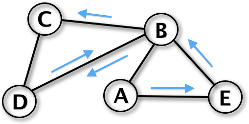
| Node Sequence (Tape) | A | E | B | D | B | C | |
|---|---|---|---|---|---|---|---|
| Time Passages () | 0 | 1 | 2 | 3 | 4 | 5 |
The second passage on node B at time is excluded in the computation of because the first passage on node B has already occurred at the second hop . However the value is added at the end of the array not-first-passage to be used later (let’s call this value ). Indeed when the first three entries of Tape are removed (loop ) and we consider the walk starting on node D the second passage in node B occurred at is now a genuine first passage. At this time, because we have removed three entries from Tape, we have and the correct number of hops between node D and the first passage on node B is given by . The value is then used in the computation of .
In Fig. 14 we show a validation of our agent-based simulation by comparing it with the result of the inversion of the matrix for a small network.
| Network | |||||||
| Synthetic Model: | |||||||
| ER | |||||||
| ER | |||||||
| ER | |||||||
| Conf. Model () | |||||||
| Conf. Model () | |||||||
| Conf. Model () | |||||||
| Conf. Model () | |||||||
| Conf. Model () | |||||||
| BA(m=3) | |||||||
| BA(m=5) | |||||||
| BA(m=20) | |||||||
| BA(m=3) | |||||||
| BA(m=5) | |||||||
| BA(m=20) | |||||||
| BA(m=20) | |||||||
| Real-world networks: | |||||||
| Gnutella(P2P) [50] | 62561 | 147877 | 4.72 | ||||
| PairsFSG [51] | |||||||
| Email URV [52] | 1133 | 5451 | |||||
| Jazz [53] | 198 | 2742 | |||||
| amazon [54] | 410236 | 2439437 | 11.89 | ||||
| USPower [55] | 4941 | 6593 | 2.66 | ||||
| SCN [41] | 12722 | 39967 | |||||
| ca-CondMath [41] | 21363 | 91286 | 8.54 | ||||
| ca-HepTh [41] | 8638 | 24806 | |||||
| ca-AstroPh [41] | 17903 | 196972 | |||||
| ca-ASTRO [41] | 13259 | 123838 | 18.68 | ||||
| ca-HepPh [56] | 11204 | 117619 | |||||
| pgp [57] | 10680 | 24316 | |||||
| C.Elegans [55] | 279 | 2287 | |||||
| bio-Yeast [58] | 2312 | 7165 | 6.20 | ||||
| www-Google [59] | 855802 | 4291352 | 10.03 | ||||
| soc-Slashdot [59] | 82168 | 582290 | 14.17 | ||||
| soc-Epinions [60] | 75877 | 405739 | 10.69 | ||||
| Actors [55] | 374511 | 1222908 | 6.53 | ||||
| wordnet [61] | 75609 | 120473 | 3.18 | ||||
| www-NotreDame [62] | 325729 | 1090108 | |||||
| www-Stanford [59] | 255265 | 1941926 | 15.21 | ||||
| www-BerkStan [59] | 654782 | 6581870 | 20.10 | ||||
| caida [56] | 26475 | 53381 | |||||
| InternetAS [36] | 11174 | 23409 | 4.19 | ||||
| USairport [63] | 1572 | 17214 | |||||
| USairports500 [64] | 500 | 2980 | |||||
| netscience.net [65] | 379 | 914 |
References
- [1] M. E. J. Newman, SIAM Review 45,, 167-256 (2003).
- [2] S. Boccaletti, V. Latora, Y. Moreno, M. Chavez and D.-U. Hwang, Phys. Rep. 424, 175 (2006).
- [3] C. Castellano, S. Fortunato and V. Loreto Rev. Mod. Phys. 81, 591 (2009).
- [4] R. Pastor-Satorras and A. Vespignani, Phys. Rev. Lett. 86, 3200 (2001).
- [5] A. Arenas, A. Diaz-Guilera, J. Kurths, Y. Moreno and C. Zhou, Phys. Rep. 469, 93 (2008).
- [6] J. D. Noh and H. Rieger, Phys. Rev. Lett. 92, 118701 (2004).
- [7] S.-J. Yang, Phys. Rev. E 71, 016107 (2005).
- [8] M. Rosvall, P. Minnhagen and K. Sneppen, Phys. Rev. E 71, 066111 (2005).
- [9] G. Ghoshal and M.E.J. Newman, Eur. Phys. J. B 58, 175 (2007)
- [10] H. Zhou, Phys. Rev. E 67, 041908 (2003).
- [11] M. Rosvall and C. T. Bergstrom, Proc. Natl. Acad. Sci. USA 105, 1118-1123 (2008).
- [12] S. Redner, A Guide to First-Passage Processes, (Cambridge University Press, Cambridge, UK, 2001).
- [13] B.D. Hughes, Random Walks and Random Environments: Random Walks, Volume 1, (Oxford University Press, Oxford, UK, 1995).
- [14] Z. Zhang, T. Shan and G. Chen, Phys. Rev. E 87, 012112 (2013).
- [15] Y.Lin and Z.Zhang, Phys. Rev. E 87, 062140 (2013).
- [16] V. Sood, S. Redner and D. ben Avraham, J. Phys. A-Math. Gen. 38, 109 (2005).
- [17] S. Condamin, O. Benichou, V. Tejedor, R. Voituriez and J. Klafter, Nature 450, 77–80 (2007).
- [18] E. Agliari, Phys. Rev. E 77, 011128 (2008).
- [19] Y. Lin, B. Wu and Z. Zhang, Phys. Rev. E 82, 031140 (2010).
- [20] B. Meyer, E. Agliari, O. Bénichou and R. Voituriez, Phys. Rev. E 85, 026113 (2012).
- [21] E. Agliari and R. Burioni, Phys. Rev. E 80, 031125 (2009).
- [22] V. Tejedor, O. Bénichou and R. Voituriez, Phys. Rev. E 80, 065104 (2009).
- [23] H. W. Lau and K. Y. Szeto, Europhys. Lett.) 90, 40005 (2010).
- [24] S. Hwang, D.-S. Lee and B. Kahng, Phys. Rev. Lett. 109, 088701 (2012).
- [25] A. Baronchelli, V. Loreto, Phys. Rev. E 73, 026103 (2006).
- [26] J. Gomez-Gardenes and V. Latora, Phys. Rev. E 78, 065102(R) (2008).
- [27] V. Zlatić, A. Gabrielli and G. Caldarelli, Phys. Rev. E 82, 066109 (2010).
- [28] S. Lee, S. H. Yook and Y. Kim, Eur. Phys. J. B 68, 277–281 (2009).
- [29] J.-C. Delvenne and A.-S. Libert, Phys. Rev. E 83, 046117 (2011).
- [30] A. Fronczak and P. Fronczak, Phys. Rev. E 80, 016107 (2009).
- [31] A. Baronchelli and R. Pastor-Satorras, Phys. Rev. E 82, 011111 (2010).
- [32] Z. Burda, J. Duda, J. M. Luck, and B. Waclaw, Phys. Rev. Lett. 102, 160602 (2009).
- [33] R. Sinatra, J. Gómez-Gardenes, R. Lambiotte, V. Nicosia and V. Latora, Phys. Rev. E 83, 030103 (2011).
- [34] Norris, James R. Markov chains. Cambridge University Press. (1998)
- [35] T. M. Cover and J. A. Thomas, Elements of Information Theory, (Wiley, 1991).
- [36] R. Pastor-Satorras, A. Vazquez and A. Vespignani, Phys. Rev. Lett. 87, 258701 (2001).
- [37] M. E. J. Newman, Phys. Rev. Lett. 89,, 208701 (2002).
- [38] M. E. J. Newman, Phys. Rev. E 67,, 026126 (2003).
- [39] C.M. Grinstead and J.L. Snell Introduction to Probability (American Mathematical Society, 1997).
- [40] E.A. Bender and E.R. Canfield, J. Combin. Theory A 24 (1978) 296.
- [41] M. E. J. Newman, Proc. Natl. Acad. Sci. USA 98, 404-409 (2001).
- [42] R. Albert, H. Jeong and A.-L. Barabasi, Nature 401, 130–131 (1999).
- [43] R. Xulvi-Brunet and I. M. Sokolov, Acta Phys. Pol. B 36, 1431 (2005).
- [44] Notice that the starting configuration model network used here has a maximum degree , which is larger than the structural cut-off of the network, as often observed in real-world networks.
- [45] L. Prignano, Y. Moreno and A. Diaz-Guilera, Phys. Rev. E 86, 066116 (2012).
- [46] U. Feige, Random Struct. Algor. 6, 433 (1995).
- [47] J. L. W. V. Jensen, Acta Math. 30 (1), 175–193 (1906).
- [48] P. Fronczak, Eur. Phys. J. B 85, 351 (2012).
- [49] Kivimäki, Ilkka, et al. “A Graph-Based Approach to Skill Extraction from Text”, Proceedings of TextGraphs-8 Graph-based Methods for Natural Language Processing, pages 79–87, October 2013, Seattle, Washington, USA.
- [50] M. Ripeanu, I. Foster, A. Iamnitchi, Mapping the Gnutella Network: Properties of Large-Scale Peer-to-Peer Systems and Implications for System Design. IEEE Internet Computing Journal, 6(1), 50-57 (2002).
- [51] Nelson, D. L., McEvoy, C. L., Schreiber, T. A. (1998). The University of South Florida word association, rhyme, and word fragment norms
- [52] R. Guimera, L. Danon, A. Diaz-Guilera, F. Giralt and A. Arenas, Phys. Rev. E 68, 065103(R), (2003).
- [53] P.Gleiser and L. Danon , Adv. Complex Syst.6, 565 (2003).
- [54] J. Leskovec, L. Adamic and B. Adamic. The Dynamics of Viral Marketing. ACM Transactions on the Web (ACM TWEB), 1(1), 2007.
- [55] D. J. Watts and S. H. Strogatz, Nature 393, 440–442 (1998).
- [56] J. Leskovec, J. Kleinberg and C. Faloutsos. “Graph Evolution: Densification and Shrinking Diameters”. ACM Transactions on Knowledge Discovery from Data (ACM TKDD), 1(1), (2007)
- [57] M. Boguña, R. Pastor-Satorras, A. Díaz-Guilera, A. Arenas, Phys. Rev. E 70, 056122 (2004)
- [58] S. Sun, L. Ling, N. Zhang, G. Li, R. Chen, Nucleic Acids Res. 31 (9), 2443 (2003).
- [59] J. Leskovec, K. Lang, A. Dasgupta, M. Mahoney, Internet Math. 6(1), 29 (2009).
- [60] M. Richardson, R. Agrawal, P. Domingos, Trust Management for the Semantic Web, In Proceedings of The Semantic Web - ISWC2003, Lecture Notes in Computer Science 2870, 351-368 (2003).
- [61] Christiane Fellbaum, editor. WordNet: an Electronic Lexical Database. MIT Press, 1998
- [62] R. Albert, H. Jeong, A.-L. Barabasi. Diameter of the World-Wide Web. Nature, 1999
- [63] Opsahl, T., 2011. Why Anchorage is not (that) important: Binary ties and Sample selection.
- [64] V. Colizza, R. Pastor-Satorras, A. Vespignani, Nat. Phys. 3, 276 (2007).
- [65] M. E. J. Newman, Phys. Rev. E 74, 036104 (2006).