Negotiating the Probabilistic Satisfaction of Temporal Logic Motion Specifications

Motion model: A Dubins vehicle ([Dub57]) is a unicycle with constant forward speed and bounded turning radius moving in a plane. In this paper, we consider a stochastic version of a Dubins vehicle, which captures actuator noise:

where $(x,y)\in\mathbb{R}^{2}$ and $\theta\in[0,2\pi)$ are the position and orientation of the vehicle in a world frame, $u$ is the control input (angular velocity before being corrupted by noise), $U$ is the control constraint set, and $\epsilon$ is a random variable modeling the actuator noise. For simplicity, we assume that $\epsilon$ is uniformly distributed on the bounded interval $[-\epsilon_{max},\epsilon_{max}]$. However, our approach works for any continuous probability distribution supported on a bounded interval. The forward speed is normalized to $1$. We denote the state of the system by $q=[x,y,\theta]^{T}\in SE(2)$.

Motivated by the fact that the optimal Dubins paths use only three inputs ([Dub57]), we assume $U=\{-1/\rho,0,1/\rho\}$, where $\rho$ is the minimum turn radius. We define

as the set of applied control inputs, i.e, the set of angular velocities that are applied to the system in the presence of noise. We assume that time is uniformly discretized (partitioned) into stages (intervals) of length $\Delta t$, where stage $k$ is from $(k-1)\Delta t$ to $k\Delta t$. The duration of the motion is finite and it is denoted by $K\Delta t$.¹¹ 1 Since PCTL has infinite time semantics, we implicitly assume after $K\Delta t$ the system remains in the state achieved at $K\Delta t$. We denote the control input and the applied control input at stage $k$ as $u_{k}\in U$ and $w_{k}\in W$, respectively.

We assume that the noise $\epsilon$ is piece-wise constant, i.e, it can only change at the beginning of a stage. This assumption is motivated by practical applications, in which a servo motor is used as an actuator for the turning angle (see e.g., [Maz04]). This implies that the applied control is also piece-wise constant, i.e., $w:[(k-1)\Delta t,k\Delta t]\rightarrow W$, $k=1,\ldots,K$, is constant over each stage.

Sensing model: We assume that the vehicle is equipped with only one sensor, which is a limited accuracy gyroscope. At stage $k$, the gyroscope returns the measured interval $[\underline{w}_{k},\overline{w}_{k}]\subset[u_{k}-\epsilon_{max},u_{k}+\epsilon_{max}]$ containing the applied control input. Motivated by practical applications, we assume that the measurement resolution of the gyroscope, i.e., the length of $[\underline{w}_{k},\overline{w}_{k}]$, is constant, and we denote it by $\Delta\epsilon$. For simplicity of presentation, we also assume that $n\Delta\epsilon=2\epsilon_{max}$, for some $n\in\mathbb{Z}^{+}$. Then, $[-\epsilon_{max},\epsilon_{max}]$ can be partitioned²² 2 Throughout the paper, we relax the notion of a partition by allowing the endpoints of the intervals to overlap. into $n$ intervals: $[\underline{\epsilon}_{i},\overline{\epsilon}_{i}]$, $i=1,\ldots,n$. We denote the set of all noise intervals as $\mathcal{E}=\{[\underline{\epsilon}_{1},\overline{\epsilon}_{1}],\ldots,[\underline{\epsilon}_{n},\overline{\epsilon}_{n}]\}$. At stage $k$, if the applied control input is $u_{k}+\epsilon$, the gyroscope will return the measured interval $[\underline{w}_{k},\overline{w}_{k}]=[u_{k}-\underline{\epsilon},u_{k}+\overline{\epsilon}],$ where $\epsilon\in[\underline{\epsilon},\overline{\epsilon}]\in\mathcal{E}$. Since $\epsilon$ is uniformly distributed:

$[\underline{\epsilon}_{i},\overline{\epsilon}_{i}]\in\mathcal{E}$, $i=1,\ldots,n$.

Environment model and specification: The vehicle moves in a static environment $X\subseteq\mathbb{R}^{2}$ in which regions of interest are present. Let $\Pi$ be a finite set of propositions satisfied at the regions in the environment. Let $[\cdot]:2^{\Pi}\rightarrow 2^{X}$ be a map such that $[\Theta]$, $\Theta\in 2^{\Pi}$, is the set of all positions in $X$ satisfying all and only propositions $\pi\in\Theta$. Inspired by a realistic scenario of an indoor vehicle leaving its charging station, we assume that the vehicle can precisely determine its initial state $q_{init}=[x_{init},y_{init},\theta_{init}]^{T}$ in a known map of the environment. Specification: In this work, we assume that the vehicle needs to carry out a motion specification expressed as a PCTL formula $\phi$ over $\Pi$:

$f\in\mathbb{Z}^{+}$, where $\forall j\in\{1,\ldots,f\}$, $\varphi_{j}$ and $\psi_{j}$ are PCTL formulas constructed by connecting properties from a set of propositions $\Pi$ using only Boolean operators in Conjunctive Normal Form (CNF) and Disjunctive Normal Form (DNF)³³ 3 A formula is CNF if it is a conjunction of clauses, where a clause is a disjunction of propositions. A formula is in DNF if it is a disjunction of clauses, where a clause is a conjunction of propositions., respectively, and $p_{j}\in[0,1]$. We assume that $\phi$ is in Negation Normal Form (NNF), i.e., Boolean operator $\neg$ appears only in front of the propositions. In order to better explain the different steps in our framework, we consider throughout the paper the following example.

Note that the proposed PCTL fragment (Eqn. (3)) can capture the usual properties of interest: reachability while avoiding regions and sequencing (see [FGKGP09]). For example, the formula $\phi:=\mathcal{P}_{max=?}[\neg{\color[rgb]{1,0,0}\pi_{u}}\wedge\neg{\color[rgb]{0,1,1}{\pi_{t1}}}\wedge\neg{\color[rgb]{1,1,0}\pi_{t2}}\mathcal{U}{\color[rgb]{0,0,1}\pi_{p}}]$ asks for the maximum probability of avoiding the unsafe, test1 and the test2 regions until a pick-up region is reached. The formula $\phi:=\mathcal{P}_{max=?}[\neg{\color[rgb]{1,0,0}\pi_{u}}\wedge\neg{\color[rgb]{0,1,1}\pi_{t1}}\wedge\neg{\color[rgb]{1,1,0}\pi_{t2}}\wedge\neg{\color[rgb]{0,1,0}\pi_{d1}}\wedge\neg{\color[rgb]{1,0,1}\pi_{d2}}\mathcal{U}({\color[rgb]{0,0,1}\pi_{p}}\wedge\mathcal{P}_{>0}[\neg{\color[rgb]{1,0,0}\pi_{u}}\wedge\neg{\color[rgb]{0,0,1}\pi_{p}}\wedge\neg{\color[rgb]{1,1,0}\pi_{t2}}\wedge\neg{\color[rgb]{0,1,0}\pi_{d1}}\wedge\neg{\color[rgb]{1,0,1}\pi_{d2}}\mathcal{U}({\color[rgb]{0,1,1}\pi_{t1}}\wedge\mathcal{P}_{>0}[\neg{\color[rgb]{1,0,0}\pi_{u}}\wedge\neg{\color[rgb]{0,0,1}\pi_{p}}\wedge\neg{\color[rgb]{0,0,1}\pi_{p}}\wedge\neg{\color[rgb]{1,1,0}\pi_{t2}}\wedge\neg{\color[rgb]{1,0,1}\pi_{d2}}\mathcal{U}{\color[rgb]{0,1,0}\pi_{d1}}])])]$ asks for the maximum probability ov visiting a pick-up, test1 and a drop-off1 region in that order.

Next, we define the satisfaction of $\phi$ (Eqn. 3) by a trajectory $q:[0,K\Delta t]\rightarrow SE(2)$ of the system from Eqn. (1). The word corresponding to a state trajectory $q(t)$ is a sequence $o=o_{1}o_{2}o_{3}\dots$, $o_{k}\in 2^{\Pi}$, $k\geq 1$, generated according to the following rules, for all $t\in[0,K\Delta t]$ and $k\in\mathbb{N}$, $k\geq 1$: 1) $(x(0),y(0))\in[o_{1}]$; 2) if $(x(t),y(t))\in[o_{k}]$ and $o_{k}\neq o_{k+1}$, then $\exists$ $t^{\prime}\geq t$ s.t. a) $(x(t^{\prime}),y(t^{\prime}))\in[o_{k+1}]$ and b) $(x(\tau),y(\tau))\notin[\pi]$, $\forall\tau\in[t,t^{\prime}]$, $\forall\pi\in\Pi\setminus(o_{k}\cup o_{k+1})$; 3) if $(x(K\Delta t),y(K\Delta t))\in[o_{k}]$ then $o_{i}=o_{k}$ $\forall i\geq k$. Informally, the word produced by $q(t)$ is the sequence of sets of propositions satisfied by the position $(x(t),y(t))$ of the robot as time evolves. A trajectory $q(t)$ satisfies PCTL formula $\phi$ iff the corresponding sequence satisfies the formula.

As time evolves and a sequence $o$ is generated, we can check what part of $\phi$ is satisfied so far. If $\mathcal{P}_{\geq p_{1}}[\varphi_{1}\mathcal{U}(\psi_{1}\wedge\ldots\wedge\mathcal{P}_{\geq p_{i}}[\varphi_{i}\mathcal{U}\psi_{i}]]$ part of $\phi$ is satisfied we say $\phi$ is satisfied up to $i$, $0\leq i\leq f$ (for more details see Sec. V-B).

Assume that at $k\Delta t$, for some $k=0,\ldots,K-1$, the motion specification is updated. Then, given $\phi$ satisfied up to $i$, $0\leq i\leq f$, the updated PCTL formula, denoted $\phi^{+}$, is obtained from $\phi$ by removing the already satisfied part of $\phi$, and then by 1) adding or removing conjunction clause from $\psi_{j}$, or 2) adding or removing a disjunction clause from $\varphi_{j}$, or 3) increasing or decreasing $p_{j}$, for any $j\in\{i,\ldots,f\}$. Formal definitions are given in Sec. V-B. To illustrate this idea consider the following example:

where $\phi^{+}$ is obtained from $\phi$ by removing the already satisfied part of $\phi$, $\mathcal{P}_{>0}[\neg{\color[rgb]{1,0,0}\pi_{u}}\wedge\neg{\color[rgb]{0,1,1}{\pi_{t1}}}\mathcal{U}\neg{\color[rgb]{1,0,0}\pi_{u}}\wedge{\color[rgb]{0,0,1}\pi_{p}}]$, and by removing the conjunction clause, $(\neg{\color[rgb]{1,0,0}\pi_{u}}\wedge{\color[rgb]{1,0,1}\pi_{d2}})$, from $\psi_{3}$. $\blacksquare$

While the vehicle moves, gyroscope measurements $[\underline{w}_{k},\overline{w}_{k}]$ are available at each stage $k$. We define a vehicle control strategy as a map that takes as input a sequence of measured intervals $[\underline{w}_{1},\overline{w}_{1}][\underline{w}_{2},\overline{w}_{2}]\ldots[\underline{w}_{k-1},\overline{w}_{k-1}]$ and returns the control input $u_{k}\in U$ at stage $k$.

We are ready to formulate the main problem that we consider in this paper:

Our approach to Problem 1 can be summarized as follows. We start by using the abstraction method presented in [CB12] as follows: by discretizing the noise interval, we define a finite subset of the set of possible applied control inputs. We use this to define a Quantized System (QS) that approximates the original system given by Eqn. (1). Next, we capture the uncertainty in the position of the vehicle and map QS to a tree-structured MDP. Then, we develop an efficient algorithm, which exploits the tree structure of the MDP, for obtaining an initial control policy that maximizes the probability of satisfying the initial specification. Next, for the PCTL formulas given by Eqn. (3) we introduce the specification update rules that guarantee the increase (or decrease) of the satisfaction probability and we develop an efficient algorithm for obtaining an updated control policy, which exploits the MDP structure, the structure of the PCTL formulas (Eqn. (3)), and reuses the initial control policy. From [CB12] it follows that each control policy can be mapped to a vehicle control strategy and that the probability that the vehicle satisfies the corresponding specification in the original environment is bounded from below by the maximum probability of satisfying the specification on the MDP.

In order to use the method presented in [CB12], we start by removing any negation operators that appear in the initial formula. To do so we use the approach presented in [FGKGP09] as follows. We introduce the extended set of propositions $\Xi_{\Pi}$. In detail, we first define two new sets of symbols $\Xi_{\Pi}^{+}=\{\xi_{\pi}|\pi\in\Pi\}$ and $\Xi_{\Pi}^{-}=\{\xi_{\neg\pi}|\pi\in\Pi\}$. Then, we set $\Xi_{\Pi}=\Xi_{\Pi}^{+}\cup\Xi_{\Pi}^{-}$. We also define a translation function pos$(\phi):\phi_{\Pi}\rightarrow\phi_{\Xi_{\Pi}}$ which takes as input a PCTL formula $\phi$ in NNF and it returns a formula pos$(\phi)$ where the occurrences of terms $\pi$ and $\neg\pi$ have been replaced by the members $\xi_{\pi}$ and $\xi_{\neg\pi}$ of $\Xi_{\Pi}$ respectively. Since we have a new set of propositions, $\Xi_{\Pi}$, we need to define a new map $[\cdot]^{\Xi_{\Pi}}:\Xi_{\Pi}\rightarrow 2^{X}$ for the interpretation of the propositions. This is straightforward: $\forall\xi\in\Xi_{\Pi}$, if $\xi=\xi_{\pi}$ then $[\xi]^{\Xi_{\Pi}}=[\pi]$, else (i.e., if $\xi=\xi_{\neg\pi}$) $[\xi]^{\Xi_{\Pi}}=X\setminus[\pi]$ (for more details see Fig. 3).

It can easily be seen that given a formula $\phi\in\Phi_{\Pi}$, a map $[\cdot]:\Pi\rightarrow 2^{X}$ and a trajectory $q(t)$ of the system from Eqn. (1), the following holds: $q(t)$ satisfies $\phi$ iff $q(t)$ satisfies pos$(\phi)$. Thus, since $\phi\in\Phi_{\Pi}$ is equivalent to the formula ${\bm{\phi}}=$pos$(\phi)$ under the maps $[\cdot]:\Pi\rightarrow 2^{X}$ and $[\cdot]^{\Xi_{\Pi}}:{\Xi_{\Pi}}\rightarrow 2^{X}$, next results are given with respect to a formula ${\bm{\phi}}\in\Phi_{\Xi_{\Pi}}$ and a map $[\cdot]^{\Xi_{\Pi}}:{\Xi_{\Pi}}\rightarrow 2^{X}$. We denote all PCTL formulas in NNF without any negation operator using bold Greek letters, e.g., ${\bm{\phi}}$, ${\bm{\phi}}^{\prime}$, ${\bm{\phi}}^{\prime}_{1}$.

At this point we have distinguished the regions that must be avoided ($\Xi_{\Pi}^{-}$) and the regions that must be reached ($\Xi_{\Pi}^{+}$).

We use $q_{k}(t)$ and $w_{k}$, $t\in[(k-1)\Delta t,k\Delta t]$, $k=1,\ldots,K$ to denote the state trajectory and the constant applied control at stage $k$, respectively. With a slight abuse of notation, we use $q_{k}$ to denote the end of state trajectory $q_{k}(t)$, i.e., $q_{k}=q_{k}(k\Delta t)$. Given a state $q_{k-1}$, the state trajectory $q_{k}(t)$ can be derived by integrating the system given by Eqn. (1) from the initial state $q_{k-1}$, and taking into account that the applied control is constant and equal to $w_{k}$. Throughout the paper, we will also denote this trajectory by $q_{k}(q_{k-1},w_{k},t)$, when we want to explicitly capture the initial state $q_{k-1}$ and the constant applied control $w_{k}$.

For each interval in $\mathcal{E}$ we define a representative value $\epsilon_{i}=\frac{\underline{\epsilon}_{i}+\overline{\epsilon}_{i}}{2}$, $i=1,\ldots,n$. i.e., $\epsilon_{i}$ is the midpoint of interval $[\underline{\epsilon}_{i},\overline{\epsilon}_{i}]$. We denote the set of all representative values as $E=\{\epsilon_{1},\ldots,\epsilon_{n}\}$. We define $W_{d}=\{u+\epsilon\text{ }|\text{ }u\in U,\epsilon\in E\}\subset W$ as a finite set of applied control inputs. Also, let $\omega:U\rightarrow W_{d}$ be a random variable, where $\omega(u)=u+\epsilon$ with the probability mass function $p_{\omega}(\omega(u)=u+\epsilon)=\frac{1}{n}$ (follows from Eqn. (2)).

Finally, we define a Quantized System (QS) that approximates the original system as follows: The set of applied control inputs in QS is $W_{d}$; for a state $q_{k-1}$ and a control input $u_{k}\in U$, QS returns

with probability $\frac{1}{n}$, where $\epsilon\in E$.

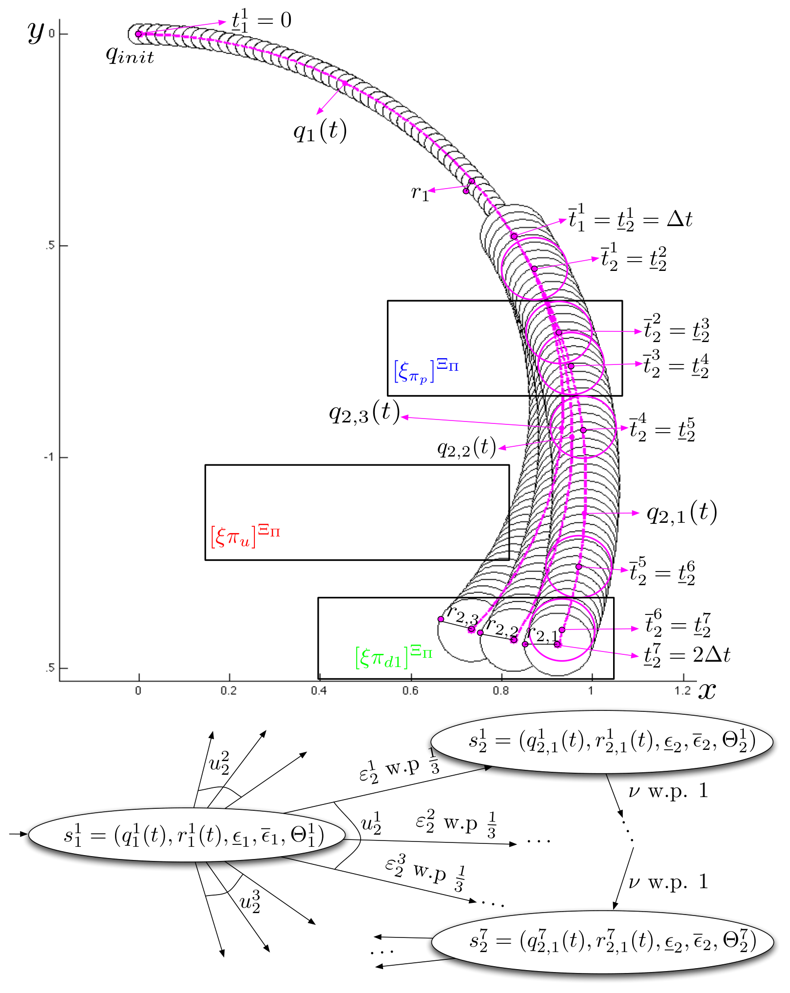
Next, we denote $u_{1}u_{2}\ldots u_{K}$, in which $u_{k}\in U$ gives a control input at stage $k$, as a finite sequence of control inputs of length $K$. Let $\Sigma_{K}$ denote the set of all such sequences. For the initial state $q_{init}$ and $\Sigma_{K}$, we define the reachability graph $G_{K}(q_{init})$ (see [LaV06] for a related definition), which encodes the set of all state trajectories originating from $q_{init}$ that can be obtained, with a positive probability, by applying sequences of control inputs from $\Sigma_{K}$ according to QS given by Eqn. (5) (an example is given in Fig. 2).

As explained before, in order to answer whether some state trajectory satisfies PCTL formula $\phi$ (Eqn. (3)), it is sufficient to know its projection in $\mathbb{R}^{2}$. Therefore, we focus only on the position uncertainty.

The position uncertainty of the vehicle when its nominal position is $(x,y)\in\mathbb{R}^{2}$ is modeled as a disc centered at $(x,y)$ with radius $r\in\mathbb{R}$, where $r$ denotes the uncertainty: $D((x,y),r)=\{(x^{\prime},y^{\prime})\in\mathbb{R}^{2}|||(x,y),(x^{\prime},y^{\prime})||\leq r\},$ where $||\cdot||$ denotes the Euclidian distance. The way we model the uncertainty along $q(t)\in G_{K}(q_{init})$ is given in [CB12]. Briefly, first, we obtain uncertainty at state $q_{k}$, denoted $r_{k}$, by using a worst case scenario assumption: if $u_{k}+\epsilon_{k}\in W_{d}$ is the applied control input for QS, the corresponding applied control input at stage $k$ for the original system was $u_{k}-\underline{\epsilon_{k}}$ or $u_{k}+\overline{\epsilon}_{k}$, where $\epsilon_{k}\in[\underline{\epsilon_{k}},\overline{\epsilon_{k}}]$. Then, we define $r:[0,K\Delta t]\rightarrow\mathbb{R}$ as an approximated uncertainty trajectory and we set $r(t)=r_{k}$, $t\in[(k-1)\Delta t,k\Delta t]$, $k=1,\ldots,K$, i.e., we set the uncertainty along the state trajectory $q_{k}(t)$ equal to the maximum value of the uncertainty along $q_{k}(t)$, which is at state $q_{k}$ (for more details see Fig. 3).

A tree-structured MDP M that models the motion of the vehicle in the environment and the evolution of the position uncertainty is defined as a tuple $(S,s_{0},Act,A,P,\Xi_{\Pi},h)$ where:
$\bullet$ $S$ is the finite set of states. The meaning of the state is as follows: $(q(t),r(t),\underline{\epsilon},\overline{\epsilon},\Theta)\in S$ means that along the state trajectory $q(t)$, the uncertainty trajectory is $r(t)$; the noise interval is $[\underline{\epsilon},\overline{\epsilon}]\in\mathcal{E}$; and $\Theta\in 2^{\Xi_{\Pi}}$ is the set of satisfied propositions along the state trajectory $q(t)$ when $r(t)$ is the uncertainty trajectory (see Fig. 3 for an example).
$\bullet$ $s_{0}=(q_{init},0,0,0,\Theta_{init})\in S$ is the initial state, where $\Theta_{init}\in 2^{\Xi_{\Pi}}$ is the set of propositions satisfied at $q_{init}$.
$\bullet$ $Act=U\cup\nu$ is the set of actions ($\nu$ is a dummy action);
$\bullet$ $A:S\rightarrow 2^{Act}$ gives the enabled actions at each state;
$\bullet$ $P:S\times Act\times S\rightarrow[0,1]$ is a transition probability function;
$\bullet$ $\Xi_{\pi}$ is the set of propositions;
$\bullet$ $h:S\rightarrow 2^{\Xi_{\pi}}$ assigns proposition from $\Xi_{\Pi}$ to states $s\in S$ according to the following rule: given $s=(q(t),r(t),\underline{\epsilon},\overline{\epsilon},\Theta)\in S$, $\forall\xi\in\Xi_{\Pi}$, $\xi\in h(s)$ iff $\xi\in\Theta$.

We generate $S$ and $P$ while building $G_{K}(q_{init})$ starting from $q_{init}$. Given $q_{k}(t)=q_{k}(q_{k-1},u_{k}+\epsilon,t)\in G_{K}(q_{init})$, and the corresponding $r_{k}(t)$, $t\in[(k-1)\Delta t,k\Delta t]$, $k=1,\ldots,K$, first, we generate a sequence $(\Theta_{k}^{1},[\underline{t}_{k}^{1},\overline{t}_{k}^{1}]),\ldots,(\Theta_{k}^{l},[\underline{t}_{k}^{l},\overline{t}_{k}^{l}])$, $l\geq 1$, where $\Theta_{k}^{i}\in 2^{\Xi_{\Pi}}$ is the set of satisfied propositions along the state trajectory $q_{k}^{i}(t)=q_{k}(t^{\prime})$, when the corresponding uncertainty trajectory is $r_{k}^{i}(t)=r_{k}(t^{\prime})$, for $t^{\prime}\in[\underline{t}_{k}^{i},\overline{t}_{k}^{i}]\subseteq[(k-1)\Delta t,k\Delta t]$, $i=1,\ldots,l$, according to the following rules:
$\bullet$ Let $\underline{t}_{k}^{1}=(k-1)\Delta t$. Then, $D((x_{k}(\underline{t}_{k}^{1}),y_{k}(\underline{t}_{k}^{1})),r_{k}(\underline{t}_{k}^{1}))\subseteq[\Theta_{k}^{1}]$ and $\overline{t}_{k}^{1}=\max_{[\underline{t}_{k}^{1},k\Delta t]}\{t|D((x_{k}(t),y_{k}(t),r_{k}(t)\subseteq[\Theta_{k}^{1}]\}$.
$\bullet$ If $D((x_{k}(t),y_{k}(t),r_{k}(t))\subseteq[\Theta_{k}^{i}]$, $t\in[\underline{t}_{k}^{i},\overline{t}_{k}^{i}]$ and $\Theta_{k}^{i+1}\neq\Theta_{k}^{i}$, then:

1. 1.

   $\exists t\geq\overline{t}_{k}^{i}$ s.t. $D((x_{k}(t),y_{k}(t),r_{k}(t))\subseteq[\Theta_{k}^{i+1}]$ and

2. 2.

   $D((x_{k}(\tau),y_{k}(\tau),r_{k}(\tau))\nsubseteq[\xi]$, $\forall\tau\in[\overline{t}_{k}^{i},t]$, $\forall\xi\in\Xi_{\Pi}\setminus(\Theta_{k}^{i}\cup\Theta_{k}^{i+1})$.

3. 3.

   $\underline{t}_{k}^{i+1}=\overline{t}_{k}^{i}$ and $\overline{t}_{k}^{i+1}=\max_{[\underline{t}_{k}^{i+1},k\Delta t]}\{t|\\ D((x_{k}(t),y_{k}(t),r_{k}(t)\subseteq[\Theta_{k}^{i+1}]\}$.

Next, for each $(\Theta_{k}^{i},[\underline{t}_{k}^{i},\overline{t}_{k}^{i}])$, $i=1,\ldots,l$, we generate a state of the MDP $s_{k}^{i}=(q_{k}^{i}(t),r_{k}^{i}(t),\underline{\epsilon},\overline{\epsilon},\Theta^{k}_{i})$ such that $q_{k}^{i}(t)=q_{k}(t^{\prime})$ and $r_{k}^{i}(t)=r_{k}(t^{\prime})$, $t^{\prime}\in[\underline{t}_{k}^{i},\overline{t}_{k}^{i}]$ and $\underline{\epsilon}$ and $\overline{\epsilon}$ are such that $\epsilon\in[\underline{\epsilon},\overline{\epsilon}]\in\mathcal{E}$. Finally, the newly generated state $s_{k}^{i}$, $i=1,\ldots l$, $l\geq 1$, is added to $S$ and the transition probability function is updated, as follows:
$\bullet$ If $i<l$, $A(s_{k}^{i})=\nu$ and $P(s_{k}^{i},\nu,s_{k}^{i+1})=1$, and otherwise, i.e., if $i=l$, $A(s_{k}^{l})=U$ and $\forall u_{k+1}\in U$, $P(s_{k}^{l},u_{k+1},s_{k+1}^{1})=\frac{1}{n}$.

The former follows from the fact that $k\Delta$ is not reached and control input for the next stage needs not to be chosen. Under dummy action $\nu$, with probability $1$, the system makes a transition to the next state in the sequence satisfying a different set of propositions. The latter follows from the fact that $k\Delta t$ is reached and the control input for the next stage needs to be chosen. Given a control input $u_{k+1}\in U$ the applied control input will be $u_{k}+\epsilon\in W_{d}$, $\epsilon\in E$, with probability $\frac{1}{n}$, and given a new state trajectory $q_{k+1}(q_{k},u_{k+1}+\epsilon,t)$ (Eqn. (5)) the first corresponding state will be $s_{k+1}^{1}$ (see Fig. 3).
$\bullet$ If the termination time is reached, we set $A(s_{k}^{i})=\nu$ and $P(s_{k}^{i},\varphi,s_{k}^{i})=1$. Such state is called a $leaf$ state.

Proof: The proof follows from the construction of the MDP. Given a current state $s\in S$ and an action $a\in A(s)$, the conditional probability distribution of future states depends only on the current state $s$, not on the sequences of events that proceed it (see the rules stated above). Thus, Markov property holds. In addition, since $\sum_{\epsilon\in\mathcal{E}}p_{\omega}(\omega(u)=u+\epsilon)=1$, it follows that $P$ is a valid transition probability function. Finally, the fact that M is a tree-structured MDP follows from the following: for each $q_{k}(t)\in G_{K}({q_{init}})$, a unique sequence of states $s_{k}^{i}$, $i=1,\ldots,l$, $l\geq 1$ is generated. Each state in that sequence has exactly one incoming transition. Thus, according to Def. 1, $M$ is a tree-structured MDP. $\blacksquare$

The proposed PCTL control synthesis is an adaptation of the approach from [LAB12]. Specifically, we exploit the tree-like structure of $M$ and develop an efficient algorithm for generating a control policy for $M$ that maximizes the probability of satisfying a PCTL formula ${\bm{\phi}}$ (Eqn. (3)).

Given a tree-structured MDP $M=(S,s_{0},A,Act,P,\Xi_{\Pi},h)$ and a PCTL formula ${\bm{\phi}}:=\mathcal{P}_{max=?}[\mathcal{P}_{\geq p_{1}}[\varphi_{1}\mathcal{U}(\psi_{1}\wedge\mathcal{P}_{\geq p_{2}}[\varphi_{2}\mathcal{U}(\psi_{2}\wedge\ldots\wedge\mathcal{P}_{\geq p_{f}}[\varphi_{f}\mathcal{U}\psi_{f}])])]]$, we are interested in obtaining the control policy $\mu_{\bm{\phi}}$ that maximizes the probability of satisfying ${\bm{\phi}}$, as well as the corresponding probability value, denoted $V_{\bm{\phi}}$, where $V_{\bm{\phi}}:S\rightarrow[0,1]$. Specifically, for $s\in S$, $\mu_{\bm{\phi}}(s)\in A(s)$ is the action to be applied at $s$ and $V_{\bm{\phi}}(s)$ is the probability of satisfying ${\bm{\phi}}$ at $s$ under control policy $\mu_{\bm{\phi}}$. To solve this problem we propose the following approach:

Step 1: Solve ${\bm{\phi}_{f}}:=\mathcal{P}_{\geq p_{f}}[\varphi_{f}\mathcal{U}\psi_{f}]$, i.e., find the set of initial states $S_{{\bm{\phi}_{f}}}$ from which ${\bm{\phi}_{f}}$ is satisfied with probably greater than or equal to $p_{f}$ and determine the corresponding control policy $\mu_{\bm{\phi}_{f}}$. To solve this problem, first, let ${\bm{\phi}_{f}^{\prime}}:=\mathcal{P}_{\max=?}[\varphi_{f}\mathcal{U}\psi_{f}]$, and compute the maximizing probabilities $V_{\bm{\phi}^{\prime}_{f}}$. This can be done by dividing $S$ into three subsets $S_{\bm{\phi}_{f}^{\prime}}^{yes}$ (states satisfying ${\bm{\phi}_{f}^{\prime}}$ with probability $1$), $S_{\bm{\phi}_{f}^{\prime}}^{no}$ (states satisfying ${\bm{\phi}_{f}^{\prime}}$ with probability $0$), and $S_{\bm{\phi}_{f}^{\prime}}^{?}$ (the remaining states):

where $\text{Sat}(\psi_{f})$ and $\text{Sat}(\varphi_{f})$ are the set of states satisfying $\psi_{f}$ and $\varphi_{f}$, respectively. The computation of maximizing probabilities for the states in $S$ can be obtained as a unique solution of the following system:

and the control policy at each state is equal to the action that gives rise to this optimal solution, i.e., $\forall s\in S$, $\mu_{\bm{\phi}_{f}^{\prime}}(s)=\text{argmax}_{a\in A(s)}\{\sum_{s^{\prime}\in S}P(s,a,s^{\prime})V_{\bm{\phi}_{f}^{\prime}}(s^{\prime})\}$.

In general (i.e., for a non tree-structured MDPs containing cycles), solving Eqn. (6) requires solving a linear programming problem ([BK08, LAB12]). For a tree-structured MDPs the solution can be obtained in a simple fashion: from each leaf state of the MDP, move backwards, by visiting parent states until $s_{0}$ is reached; at each state in $S_{\bm{\phi}_{f}^{\prime}}^{?}$ perform maximization from Eqn. (6). The fact that $M$ contains no cycles is sufficient to see that the procedure stated above will result in maximizing probabilities.

The state formula ${\bm{\phi}_{f}}$ requires to reach a state in $\text{Sat}(\psi_{f})$ by going through states in $\text{Sat}(\varphi_{f})$ with probability greater than or equal to $p_{f}$. Thus, $\forall s\in S$ s.t. $V_{\bm{\phi}_{f}^{\prime}}(s)<p_{f}$ we set $V_{\bm{\phi}_{f}}(s)=0$, and otherwise, i.e., $\forall s\in S$ s.t. $V_{\bm{\phi}_{f}^{\prime}}(s)\geq p_{f}$ we set $V_{\bm{\phi}_{f}}(s)=V_{\bm{\phi}_{f}^{\prime}}(s)$. Finally, $\forall s\in S$, $\mu_{\bm{\phi}_{f}}(s)=\mu_{\bm{\phi}_{f}^{\prime}}(s)$ and the set of initial states is $S_{{\bm{\phi}_{f}}}=\{s\in S|V_{\bm{\phi}_{f}}(s)>0\}.$

Step 2: Solve ${\bm{\phi_{f-1}}}:=\mathcal{P}_{\geq p_{f-1}}[\varphi_{f}\mathcal{U}(\psi_{f-1}\wedge{\bm{\phi}_{f}})]$, i.e., find the set of initial states $S_{{\bm{\phi_{f-1}}}}$ from which ${\bm{\phi_{f-1}}}$ is satisfied with probability greater than or equal to $p_{f-1}$. To solve this problem, again, begin by solving ${\bm{\phi_{f-1}^{\prime}}}:=\mathcal{P}_{\max=?}[\varphi_{f-1}\mathcal{U}(\psi_{f-1}\wedge{\bm{\phi}_{f}})]$. Start by dividing $S$ into three subsets:

Note that, $S_{\bm{\phi}_{f-1}^{\prime}}^{yes}$ is the set of states satisfying $\psi_{f-1}$ intersected with $S_{{\bm{\phi}_{f}}}$. Next, perform the same procedure as in Step 1 for obtaining $V_{\bm{\phi}_{f-1}}$, $\mu_{\bm{\phi}_{f-1}}$ and $S_{{\bm{\phi_{f-1}}}}$.

References

- [BK08] C. Baier and J. P. Katoen. Principles of Model Checking. MIT Press, 2008.
- [BKV10] A. Bhatia, L.E. Kavraki, and M.Y. Vardi. Sampling-based Motion Planning with Temporal Gaoals. In International Conference on Robotics and Automation (ICRA) 2010, pages 2689–2696, 2010.
- [CB12] I. Cizelj and C. Belta. Probabilistically Safe Control of Noisy Dubins Vehicles. In IEEE Intelligent Robots and Systems (IROS) Conference, 2012, pages 2857 –2862, October 2012.
- [CGP99] E. Clarke, O. Grumberg, and D. A. Peled. Model Checking. The MIT Press, 1999.
- [DLB12] X. C. Ding, M. Lazar, and C. Belta. Receding Horizon Temporal Logic Control for Finite Deterministic Systems. In American Control Conference (ACC) 2012, June 2012.
- [Dub57] L. E. Dubins. On curves of minimal length with a constraint on average curvature, and with prescribed initial and terminal positions and tangents. American Journal of Mathematics, 79(3):497–516, 1957.
- [Fai11] G. Fainekos. Revising Temporal Logic Specifications for Motion Planning. In nternational Conference on Robotics and Automation (ICRA) 2011, pages 40–45, 2011.
- [FGKGP09] G. Fainekos, A. Girard, H. Kress-Gazit, and G.J. Pappas. Temporal Logic Motion Planning for Dynamic Robots. Automatica, 45(2):343–352, 2009.
- [GKP11] N. Ghita, M. Kloetzer, and O. Pastravanu. Probabilistic Car-Like Robot Path Planning from Temporal Logic Specifications. In International Conference on System Theory, Control, and Computing (ICSTCC), 2011, pages 1–6, 2011.
- [JKG12] B. Johnson and H. Kress-Gazit. Probabilistic Guarantees for High-Level Robot Behavior in the Presence of Sensor Error. Autonomous Robots, 33(3):309–321, 2012.
- [KB08a] M. Kloetzer and C. Belta. Dealing with Non-Determinism in Symbolic Control. In Hybrid Systems: Computation and Control (HSCC) 2008, pages 287–300, 2008.
- [KB08b] M. Kloetzer and C. Belta. A Fully Automated Framework for Control of Linear Systems from Temporal Logic Specifications. IEEE Transactions on Automatic Control, 53(1):287 –297, 2008.
- [KF08] S. Karaman and E. Frazzoli. Vehicle Routing Problem with Metric Temporal Logic Specifications. In Conference on Decision and Control (CDC) 2008, pages 3953 –3958, 2008.
- [KGFP07] H. Kress-Gazit, G. E. Fainekos, and G. J. Pappas. Where’s Waldo? Sensor-Based Temporal Logic Motion Planning. In International Conference on Robotics and Automation (ICRA) 2007, pages 3116–3121, 2007.
- [KNP04] M. Kwiatkowska, G. Norman, and D. Parker. Probabilistic symbolic model checking with PRISM: A hybrid approach. International Journal on Software Tools for Technology Transfer, 6(2):128–142, 2004.
- [LAB12] M. Lahijanian, S. B. Andersson, and C. Belta. Temporal Logic Motion Planning and Control With Probabilistic Satisfaction Guarantees. IEEE Transactions on Robotics, 28(2):396 –409, 2012.
- [LaV06] S. M. LaValle. Planning Algorithms. Cambridge University Press, Cambridge, U.K., 2006.
- [Maz04] M. Mazo. Robust Area Coverage using Hybrid Control. In TELEC’04, Santiago de Cuba, Cuba, 2004.
- [WTM09] T. Wongpiromsarn, U. Topcu, and R. M. Murray. Receding Horizon Temporal Logic Planning for Dynamical Systems. In Conference on Decision and Control (CDC) 2009, pages 5997 –6004, 2009.