Scalable Eventually Consistent Counters over Unreliable Networks

Paulo Sérgio Almeida Carlos Baquero Email: {psa,cbm}@di.uminho.pt Affiliation: HASLab, INESC Tec & Universidade do Minho

Abstract

Counters are an important abstraction in distributed computing, and play a central role in large scale geo-replicated systems, counting events such as web page impressions or social network “likes”. Classic distributed counters, strongly consistent, cannot be made both available and partition-tolerant, due to the CAP Theorem, being unsuitable to large scale scenarios. This paper defines Eventually Consistent Distributed Counters (ECDC) and presents an implementation of the concept, Handoff Counters, that is scalable and works over unreliable networks. By giving up the sequencer aspect of classic distributed counters, ECDC implementations can be made AP in the CAP design space, while retaining the essence of counting. Handoff Counters are the first CRDT (Conflict-free Replicated Data Type) based mechanism that overcomes the identity explosion problem in naive CRDTs, such as G-Counters (where state size is linear in the number of independent actors that ever incremented the counter), by managing identities towards avoiding global propagation and garbage collecting temporary entries. The approach used in Handoff Counters is not restricted to counters, being more generally applicable to other data types with associative and commutative operations.

1 Introduction

A counter is one of the most basic and important abstractions in computing. From the small-scale use of counter variables in building data-types, to large-scale distributed uses for counting events such as web page impressions, banner clicks or social network “likes”. Even in a centralized setting, the increment operation on a counter is problematic under concurrency, being one of the examples most used to illustrate the problems that arise if a load, add one and store are not atomic. In a distributed setting things are much worse, due to the absence of shared memory, possibly unreliable communication (message loss, reordering or duplication), network partitions or node failures.

If one has a strongly consistent distributed database with support for distributed transactions counters can be trivially obtained. Unfortunately, such databases are not appropriate for large-scale environments with wide-area replication, high latency and possible network partitions. A naive counter obtained through a “get, add one, and put” transaction will not scale performance-wise to a wide-area deployment with many thousands of clients.

The CAP theorem [4, 10] says that one cannot have Consistency, Availability, and Partition-tolerance together; one must choose at most two of these three properties. Therefore, to have an always-available service under the possibility of partitions (that in world-wide scenarios are bound to happen from time to time), distributed data stores such as Dynamo [7], Cassandra [18] and Riak [17] have been increasingly choosing to go with AP (availability and partition-tolerance) and give up strong consistency and general distributed transactions, in what has become known as the NoSQL movement.

With no support for strong consistency and distributed transactions, and an API mostly based on simple get and put operations, obtaining a “simple” counter becomes a problem. NoSQL data stores like Cassandra have been trying to offer counters natively with an increment operation in the API, something that has revealed a non-trivial problem, involving many ad hoc evolutions. The current state in Cassandra is well summarized by [12]: “The existing partitioned counters remain a source of frustration for most users almost two years after being introduced. The remaining problems are inherent in the design, not something that can be fixed given enough time/eyeballs.”

An approach towards obtaining provably correct eventually consistent implementations of data types such as counters are the so called CRDTs: Conflict-free Replicated Data Types [23]. The idea is that each node keeps a CRDT (a replica) that can be locally queried or operated upon, giving availability even under partitions, but providing only eventual consistency: queries can return stale values, but if “enough” messages go through, then all nodes will converge to the correct value. CRDT-based data types (the state-based ones) can be built to trivially tolerate unreliable communication. They are designed so that duplicates or non-FIFO communication are not a problem.

CRDTs are not, however, the silver bullet they are sometimes assumed to be. A problem that can easily arise in CRDTs is scalability. This problem is easy to explain: the CRDT approach envisions a CRDT per participating entity; in many CRDTs each entity needs to have a unique identity, and many CRDTs are made to work by keeping maps from participating entities ids to some value; the set of keys in these maps will keep growing along time, as more entities participate, preventing scalability.

This means that practical CRDT-based approaches to counters involving some server nodes and possibly many clients will exclude clients from the entities having CRDTs, having them server-side only. This will solve the scalability problem and allow unreliable communication between servers, but will not solve the fault-tolerance problem in the client-server interaction. This is because a basic problem with counters is that the increment operation is not idempotent; therefore, an increment request by a client (which itself does not keep a CRDT) cannot just be re-sent to the server in case there is no acknowledgment. This problem is well recognized by practitioners, as can be seen by, e.g., [19].

If one looks at theory of distributed counting, a substantial amount of work has been done, namely Software Combining Trees [29, 11], Counting Networks [1], Diffracting Trees [24] and Counting Pyramid [28] (and many variants of these, specially of counting networks). However, all these works address a strongly consistent definition of counter, as a data type that provides a single “fetch-and-increment” operation in the sense of [25]. Although an unquestionably powerful abstraction (e.g., to generate globally unique sequence numbers), it is indeed too powerful to be implemented while providing availability under unreliable communication with possible partitions. The focus of these works is scalability (mainly avoiding contention or bottlenecks) and not fault-tolerance. While some aspects like wait-freedom are addressed, to tolerate failures of processes, tolerance to message loss or component failure (e.g., a balancer in the case of counting networks) is not addressed. This means that the applicability of these mechanisms is mostly in tightly-coupled, low-latency, failure-free environments, such as multiprocessors, serving as scalable alternatives to lock-based counter implementations, as discussed in [15].

The remainder of this paper is organized as follows: Section 2 briefly revisits classic strongly consistent distributed counters, and explains why they are not suitable for large-scale AP scenarios. In Section 3 we propose a definition of Eventually Consistent Distributed Counters (ECDC), stating both safety and liveness conditions. Section 4 describes a naive eventually consistent CRDT-based counter, that is AP in unreliable networks, and explains its scalability problems; it also discusses in more detail the problems that arise if these CRDTs are restricted to server-side. In Section 5 we present Handoff Counters, our new CRDT-based mechanism that implements eventually consistent counters that is simultaneously reliable, available and partition-tolerant under unreliable networks, and scalable in the number of entities (both active and already terminated). Section 6 contains formal correctness proofs for the mechanism. In Section 7 we address some practical implementation issues. In Section 8 we discuss how the handoff mechanism proposed can be applied to more general scenarios, beyond simple counters, to commutative monoids having an associative and commutative operation, and conclude in Section 10.

2 Classic Distributed Counters

In most papers about distributed counters, e.g., [1, 24, 28], a counter is an abstract data type that provides a fetch-and-increment operation (increment for short), which returns the counter value and increments it. The basic correctness criteria is usually: a counter in a quiescent state (when no operation is in progress) after $n$ increments have been issued will have returned all values from $0$ to $n-1$ with no value missing or returned twice. I.e., when reaching a quiescent state, all operations so far must have behaved as if they have occurred in some sequential order, what is known as quiescent consistency [1]. Some counter mechanisms, e.g., [28], enforce the stronger linearizability [16] condition, which ensures that, whenever a first increment returns before a second one is issued, the first returns a lower value than the second.

Even forgetting the stronger variants that enforce linearizability, classic distributed counters providing quiescent consistency are too strongly consistent if one is aiming for availability and partition tolerance. For classic distributed counters we have the following result for deterministic algorithms, with a trivial proof, which is nothing more than an instantiation of the CAP theorem:

Proposition 2.1.

A quiescently consistent fetch-and-increment counter cannot be both available and partition tolerant.

Proof.

Suppose a network with two nodes $u$ and $v$ , and a run $A$ where they are partitioned. Assume an increment is issued at node $u$ at time $t_{1}$ and no other operations are in progress. As the counter is available and partition tolerant, it will eventually return at some later time $t_{2}$ . Because the system is in a quiescent state after $t_{2}$ , this increment must have returned $0$ . Suppose an increment is then issued at node $v$ at some later time $t_{3}>t_{2}$ . For the same reasons, this increment will eventually return, the system becomes quiescent again, and the returned value must, therefore, be $1$ . But as no messages got through between $u$ and $v$ , this run is indistinguishable by $v$ from a run $B$ in which $u$ does not exist and only a single increment is issued by $v$ . In run $B$ , $v$ will, therefore, behave the same as in run $A$ and return the same value $1$ , which contradicts the requirement for run $B$ that a single increment in the whole run should have returned $0$ after reaching quiescence. ∎

This simply formalizes the intuition that it is not possible to generate globally unique numbers forming a sequence in a distributed fashion without communication between the nodes involved.

3 Eventually Consistent Distributed Counters

Given the too strongly consistent nature of classic distributed counters, to achieve availability and partition tolerance a weaker variant of distributed counters needs to be devised. In this section we define such a variant, that we call eventually consistent distributed counters (ECDC).

Classic counters offer a two-in-one combination of two different features: 1) keeping track of how many increments have been issued; 2) returning globally unique values. While undoubtedly powerful, this second feature is the problematic one if aiming for AP.

For many practical uses of counters (in fact what is being offered in NoSQL data stores like Cassandra and Riak) one can get away with not having the second feature, and having a counter as a data type that can be used to count events, by way of an increment operation, which does not return anything, and an independent fetch operation, which returns the value of the counter. This splitting makes clear that one is not aiming for obtaining globally unique values (fetch can return the same value several times), and one can start talking about possibly returning stale values. Having two independent operations, one to mutate and the other to report, as opposed to a single atomic fetch-and-increment, corresponds also to the more mundane conception of a counter, and to what is required in a vast number of large scale practical uses, where many participants increment a counter while others (typically less, usually different) ask for reports.

It will be possible to obtain available and partition tolerant eventually consistent counters, by allowing fetch to return something other than the more up-to-date value. Nevertheless, we need concrete correctness criteria for ECDC. We have devised three conditions. Informally:

•

A fetch cannot return a value greater than the number of increments issued so far.
•

At a given node, a fetch should return at least the sum of the value returned by the previous fetch (or 0 if no such fetch was issued) plus the number of increments issued by this node between these two fetches.
•

All increments issued up to a given time will be reported eventually at a later time (when the network has allowed enough messages to go through).

The first two criteria can be thought of as safety conditions. The first, not over-counting, is the more obvious one (and also occurs in classic distributed counters, as implied by their definition). The second is a local condition on session guarantees [26], analogous to having read-your-writes and monotonic-read, common criteria in eventual consistency [27]. The third is a liveness condition, which states that eventually, if network communication allows, all updates are propagated and end up being reported. It implies namely that if increments stop being issued, eventually fetch will report the correct counter value, i.e., the number of increments. We will now clarify the system model, and subsequently formalize the above correctness criteria for ECDC.

3.1 System Model

Consider a distributed system with nodes containing local memory, with no shared memory between them. Any node can send messages to any other node. The network is asynchronous, there being no global clock, no bound on the time it takes for a message to arrive, nor bounds on relative processing speeds. The network is unreliable: messages can be lost, duplicated or reordered (but are not corrupted). Some messages will, however, eventually get through: if a node sends infinitely many messages to another node, infinitely many of these will be delivered. In particular, this means that there can be arbitrarily long partitions, but these will eventually heal.

Nodes have access to stable storage; nodes can crash but eventually will recover with the content of the stable storage as at the time of the crash. Each node has access to a globally unique identifier.

As we never require that data type operations block waiting for other operations or for message reception, they are modeled as single atomic actions. (In I/O Automata [20] parlance, we will use a single action as opposed to a pair $\mathop{\hbox{$\mathsf{opStart}$}}\nolimits$ (input action), and $\mathop{\hbox{$\mathsf{opEnd}$}}\nolimits(r)$ (output action) “returning” $r$ ). This allows us to use $\mathop{\hbox{$\mathsf{op}$}}\nolimits_{i}^{t}$ to mean that operation op was performed by node $i$ at time $t$ , and in the case of fetch also for the result of that operation. The actions we use are $\mathop{\hbox{$\mathsf{fetch}$}}\nolimits_{i}$ and $\mathop{\hbox{$\mathsf{incr}$}}\nolimits_{i}$ for the data type operations, and $\mathop{\hbox{$\mathsf{send}$}}\nolimits_{i,j}(m)$ and $\mathop{\hbox{$\mathsf{receive}$}}\nolimits_{i,j}(m)$ for message exchange.

3.2 Formal Correctness Criteria for ECDC

An eventually consistent distributed counter is a distributed abstract data type where each node can perform operations $\mathop{\hbox{$\mathsf{fetch}$}}\nolimits$ (returning an integer) and $\mathop{\hbox{$\mathsf{incr}$}}\nolimits$ (short for increment), such that the following conditions hold (where $\left|\ \right|$ denotes set cardinality and $\_$ the unbound variable, matching any node identifier; also, for presentation purposes, we assume an implicit $\mathop{\hbox{$\mathsf{fetch}$}}\nolimits_{\_}^{0}=0$ at time 0 by all nodes). For any node $i$ , and times $t,t_{1},t_{2}$ , with $t_{1}<t_{2}$ :

Fetch bounded by increments:

\mathop{\hbox{$\mathsf{fetch}$}}\nolimits_{i}^{t}\leq\left|\{\mathop{\hbox{$\mathsf{incr}$}}\nolimits_{\_}^{t^{\prime}}|t^{\prime}<t\}\right|,

Local monotonicity:

\mathop{\hbox{$\mathsf{fetch}$}}\nolimits_{i}^{t_{2}}-\mathop{\hbox{$\mathsf{fetch}$}}\nolimits_{i}^{t_{1}}\geq\left|\{\mathop{\hbox{$\mathsf{incr}$}}\nolimits_{i}^{t^{\prime}}|t_{1}<t^{\prime}<t_{2}\}\right|,

Eventual accounting:

\exists t^{\prime}\geq t.\forall j.\mathop{\hbox{$\mathsf{fetch}$}}\nolimits_{j}^{t^{\prime}}\geq\left|\{\mathop{\hbox{$\mathsf{incr}$}}\nolimits_{\_}^{t^{\prime\prime}}|t^{\prime\prime}<t\}\right|.

These criteria, specific to counters, can be transposed to more general consistency criteria, namely they imply the analogous for counters of:

Eventual Consistency: From [27] “[It] guarantees that if no new updates are made to the object, eventually all accesses will return the last updated value.”. Eventual accounting is stronger than eventual consistency: it does not require increments to stop, but clearly leads to eventual consistency if increments do stop. All CRDTs include this consistency criteria [23].
Read-your-writes: From [26] “[It] ensures that the effects of any Writes made within a session are visible to Reads within that session.”. The analogous of this property, substituting increments for writes, is implied by local monotonicity: in a session where a process issues increments to a given node, at least the effect of those increments is seen by further fetches by that process.
Monotonic-reads: Defined in [26] and using the formulation in [27] “If a process has seen a particular value for the object, any subsequent accesses will never return any previous values.”. This property is also obtained by local monotonicity.

4 Naive CRDT-based Counters

A state-based CRDT amounts to a replica that can be locally queried or updated; it directly provides availability and partition tolerance, as all client-visible data type operations are performed locally, with no need for communication. Information is propagated asynchronously, by sending the local state to other nodes (e.g., using some form of gossip [8]); the receiving node performs a merge between the local and the received CRDT. CRDTs are designed so that: their abstract state forms a join semilattice (a partially ordered set for which there is a defined least upper bound for any two elements, see, e.g., [6]); the merge operation amounts to performing a mathematical join of the correspondent abstract states, deriving their least upper bound; every data type operation is an inflation that moves the state to a larger value (i.e., $\forall x.f(x)\geq x$ ). This means that merges can be performed using arbitrary communication patterns: join is associative, commutative and idempotent; duplicates are, therefore, not a problem and in doubt of message loss, a message can be resent and possibly re-merged; old messages received out-of-order are also not a problem. CRDTs solve, therefore, the problem of unreliable communication for data types that conform to their design.

The CRDT concept can be used to trivially obtain an ECDC. The local state will amount to a version-vector [21]: a map of node ids to non-negative integers. When a node wants to perform an increment, it increments the entry corresponding to its unique identifier (or adds an entry mapped to one if the id is not mapped). The fetch is obtained by adding all integers in the map. The merge operation also corresponds to reconciliation of version-vectors: maps are merged by performing a pointwise maximum (each key becomes mapped to the maximum of the corresponding values, assuming absent keys are implicitly mapped to 0).

It is easy to see that these version-vector based counters respect the criteria for ECDC. The fetch results from adding values that result from increments performed, being bounded by the number of increments; local increments are immediately accounted; as increments by different nodes are performed in disjoint entries, if each CRDT is propagated and merged to every other one, all will converge to a CRDT that stores the exact number of increments performed by each node in the corresponding map entry; therefore, all increments are eventually accounted.

4.1 The Scalability Problem of Client-side CRDTs

Counters implemented as version-vectors, although meeting all criteria for ECDC over unreliable networks, suffer from serious scalability problems. Consider a network in which many nodes (clients) perform operations, while others (servers) allow information propagation and keep durable storage after client nodes have ceased from participating.

The pure CRDT approach assumes that all participating entities have a CRDT. In this case, each participating node (both clients and servers) will introduce its id in the map. Over time the map will grow to unreasonable sizes, making both the storage space and communication costs (of transmitting the map to be merged on the other node) unbearable. The worst aspect is that the size does not depend only on the currently participating clients: it keeps growing, accumulating all ids from past clients that have already stopped participating. This means that naive client based CRDTs are not scalable and not usable in some relevant practical cases.

4.2 The Availability Problem of Server-side CRDTs

Due to the above scalability problem, current version-vector based counters (e.g., in Cassandra or Riak) do not use the pure CRDT approach, but use CRDTs server-side only. This means that only a relatively small number of nodes (the servers) hold CRDTs, while clients use remote invocations to ask a server to perform the operation. Server-side CRDTs allow unreliable communication between servers, including partitions (e.g., between data-centers). However, the problem of unreliable communication between client and server remains.

As the increment operation is not idempotent, it cannot be simply reissued if there is doubt whether it was successful. In practice, this leads to the use of remote invocations over connection-oriented protocols (e.g., TCP [5]) that provide reliable communication. This only partially solves the problem: a sequence of acknowledged increments is known to have been applied exactly-once, but if the last increment is not acknowledged and the connection timeouts, this last increment is not known to have been successfully applied, but cannot be reissued using a new connection, to the same or a different server, as it could lead to over-counting.

Attempts to circumvent this reliability problem through a general data-type-agnostic communication layer bring back scalability and/or availability problems. If an infinite duration connection incarnation is maintained for each client, where no operation can fail due to a timeout, this will imply stable server state to manage each client connection, leading to state explosion in servers, as clients cannot be forgotten. This because there is no protocol that gives reliable message transfer within an infinite incarnation for general unbounded capacity (e.g., wide-area networks) non-FIFO lossy networks that does not need stable storage between crashes [2, 9]. This problem can be overcome by never failing due to a timeout, but allowing connections to be closed if there are no pending requests and the connection close handshake is performed successfully (e.g., before a partition occurs). With a three-way handshake an oblivious protocol is possible [3], with no need to retain connection specific information between incarnations, but only a single unbounded counter for the whole server.

With this last approach, the size of stable server state is not a problem in practice, but the reliability problem is overcome at the cost of availability: given a partition, a pending request will never fail due to a time-out, but the client that has issued a request to a given server will be forced to wait unboundedly for the result from that server, without being able to give up waiting and continue the operation using a different server.

These problems can be summarized as: the use of a general purpose communication mechanism to send non-idempotent requests can provide reliability at the cost of availability. Our data-type specific mechanism overcomes this problem by allowing client-side CRDTs which are scalable.

5 Handoff Counters

In this section we present a novel CRDT based counter mechanism, which we call Handoff Counters, that meets the ECDC criteria, works in unreliable networks and, as opposed to simple version vector CRDT counters, is scalable. The mechanism allows arbitrary numbers of nodes to participate and adopts the CRDTs everywhere philosophy, without distinguishing clients and servers, allowing an operation (fetch or increment) to be issued at any node.

It addresses the scalability issues (namely the id explosion in maps) by: assigning a tier number (a non negative integer) to each node; promoting an hierarchical structure, where only a small number of nodes are classified as tier 0; having “permanent” version vector entries only in (and for) tier 0 nodes, therefore, with a small number of entries; having a handoff mechanism which allows a tier $n+1$ “client” to handoff values to some tier $n$ “server” (or to any smaller tier node, in general); making the entries corresponding to “client” ids be garbage-collected when the handoff is complete. Figure 1 illustrates a simple configuration, with end-client nodes connecting to tier 1 nodes in their regional datacenters.

Example 5.1.

Even though no formal client/server distinction is made, a typical deployment scenario would be having, e.g., two (for redundancy) tier 0 nodes per data-center, devoted to inter-datacenter communication, a substantial, possibly variable, number of tier 1 server nodes per datacenter, and a very large number of tier 2 nodes in each datacenter. The datastore infrastructure would be made up of tier 0 and 1 nodes, while tier 2 nodes would be the end-clients (application server threads handling end-client connections or code running at the end-clients) connecting to tier 1 nodes in a datacenter. More tiers can be added in extreme cases, but this setup will be enough for most purposes: e.g., considering 5 datacenters, 50 tier 1 nodes per datacenter, each serving 1000 concurrent tier 2 clients, will allow 250000 concurrent clients; in this case the “permanent” version vectors will have 10 entries.

Refer to caption — Figure 1: A simple configuration with three tiers and two datacenters.

The mechanism involves three aspects: the handoff, which migrates accounted values towards smaller tiers, making all increments eventually be accounted in tier 0 nodes; classic version vector dissemination and merging between tier 0 nodes; top-down aggregation from tier 0 to bottom-tier nodes, to provide a best-effort monotonic estimate of the counter value.

Most complexity of the mechanism is related to achieving the handoff without violating correctness under any circumstances over unreliable networks, while allowing garbage-collection in typical runs. Other design aspects were considered, in addition to strictly achieving ECDC, namely:

•

an end-client (maximum tier node) is typically transient; it should be able to know if locally issued increments have already been handed-off, so that it can stop the interaction and terminate;
•

there should be no notion of session or affinity; a tier $n+1$ node $u$ that started exchanging messages with a tier $n$ node $v$ , should be able to switch to another tier $n$ node $w$ at any time, e.g., if no message arrives and $u$ suspects that $v$ has crashed or there is a network partition between $u$ and $v$ , but $u$ is an end-client that wants to be sure its locally accounted increments have been handed-off to some server before terminating.

5.1 Network Topology

Handoff counters can be used with many different network topologies. The simplest one is to assume a fully connected graph, where any node can send messages to any other node. In general, handoff counters can work with less connectivity. The assumptions that we make about network topology for the remainder of the paper are:

•

Each link is bidirectional.
•

The network restricted to tier 0 nodes is a connected sub-network.
•

For each node $u$ , there is a path from $u$ to a tier 0 node along a strictly descending chain of tiers.
•

If a tier node $u$ is linked to two smaller tier nodes $v$ and $w$ , then there is also a link between $v$ and $w$ .

These assumptions allow version vector dissemination in tier 0 nodes, while also allowing a client $u$ to start by exchanging messages with a server $v$ and later switching to a server $w$ if $v$ becomes unresponsive. These assumptions are met by Example 5.1 and by the Figure 1 topology, where inter-datacenter communication is performed by tier 0 nodes, and where communication between tier 1 nodes or between tier $n+1$ and tier $n$ nodes needs only be attempted within each datacenter. It should be emphasized that these assumptions reflect only what communications are attempted, and can be thought of as the rules for forming a communication overlay; any of these links may be down for some time, even possibly incurring in temporary network partitions.

5.2 Distributed Algorithm

A benefit of adopting the CRDT approach is not needing a complex distributed algorithm – the complexity is transferred to the CRDT. To achieve correctness, basically any form of gossip can be used, where each node keeps sending its state instance to randomly picked neighbors, and each node upon receiving an instance merges it with the local one. To address efficiency, concerns like the choice of neighbors to communicate will need attention; we address such concerns in Section 7.

To describe both the mechanism and its correctness proofs we consider Algorithm 1 to be used, with operations defined in Figures 4 and 5. In this algorithm, each node $i$ has a local replica $C_{i}$ , which is an instance of the Handoff Counter CRDT. A CRDT replica is initialized using the globally unique node id and the node tier. The local operations $\mathop{\hbox{$\mathsf{fetch}$}}\nolimits_{i}$ and $\mathop{\hbox{$\mathsf{incr}$}}\nolimits_{i}$ are delegated to the corresponding CRDT ones. Each node periodically picks a random neighbor $j$ and sends it the local instance. Upon receiving an instance $C_{j}$ through a link $(j,i)$ , it is merged with the local one, through the CRDT merge operation. The algorithm is quite trivial, all effort being delegated to the Handoff Counter data type, namely through its $\mathop{\hbox{$\mathsf{init}$}}\nolimits$ , $\mathop{\hbox{$\mathsf{fetch}$}}\nolimits$ , $\mathop{\hbox{$\mathsf{incr}$}}\nolimits$ and $\mathop{\hbox{$\mathsf{merge}$}}\nolimits$ operations.

Regarding fault tolerance, the state $C_{i}$ is assumed to be stored in stable storage, and assigning to it is assumed to be an atomic operation. This means that temporary variables used in computing a data-type operation do not need to be in stable storage, and an operation can crash at any point before completing, in which case $C_{i}$ will remain unchanged. The functional style used in defining the CRDT and algorithm emphasizes this aspect.

1 constants:

i

, globally unique node id

t_{i}

, node

i

tier

n_{i}

, set of neighbors

5 state:

C_{i}

, handoff counter data type; initially,

C_{i}=\mathop{\hbox{$\mathsf{init}$}}\nolimits(i,t_{i})

7 on

\mathop{\hbox{$\mathsf{fetch}$}}\nolimits_{i}

8 return

\mathop{\hbox{$\mathsf{fetch}$}}\nolimits(C_{i})

9 on

\mathop{\hbox{$\mathsf{incr}$}}\nolimits_{i}

C_{i}:=\mathop{\hbox{$\mathsf{incr}$}}\nolimits(C_{i})

11 on

\mathop{\hbox{$\mathsf{receive}$}}\nolimits_{j,i}(C_{j})

C_{i}:=\mathop{\hbox{$\mathsf{merge}$}}\nolimits(C_{i},C_{j})

13 periodically

14 let

j=\mathop{\hbox{$\mathsf{random}$}}\nolimits(n_{i})

\mathop{\hbox{$\mathsf{send}$}}\nolimits_{i,j}(C_{i})

Algorithm 1 Distributed algorithm for a generic node

i

5.3 Handoff Counter Data Type

Unfortunately, the Handoff Counter data type is not so trivial. On one hand, a server which is receiving counter values from a client should be able to garbage collect client specific entries in its state; on the other hand, neither duplicate or old messages should lead to over-counting, nor lost messages lead to under-counting. Towards this, a handoff counter has state that allows a 4-way handshake in which some accounted value (a number of increments) is moved reliably from one node to the other. To understand the essence of the mechanism, the steps when a node $i$ is handing-off some value to a node $j$ , when no messages are lost, are the following, as exemplified in Figure 2:

1.

Node $i$ sends its $C_{i}$ to node $j$ ; node $j$ does $C^{\prime}_{j}:=\mathop{\hbox{$\mathsf{merge}$}}\nolimits(C_{j},C_{i})$ ; the resulting $C^{\prime}_{j}$ has a slot created for node $i$ ;
2.

Node $j$ sends $C^{\prime}_{j}$ to $i$ ; node $i$ performs $C^{\prime}_{i}:=\mathop{\hbox{$\mathsf{merge}$}}\nolimits(C_{i},C^{\prime}_{j})$ ; the resulting $C^{\prime}_{i}$ has a token specifically created for that slot, into which the locally accounted value has been moved;
3.

Node $i$ sends $C^{\prime}_{i}$ to node $j$ ; node $j$ does a $C^{\prime\prime}_{j}:=\mathop{\hbox{$\mathsf{merge}$}}\nolimits(C^{\prime}_{j},C^{\prime}_{i})$ ; this merge, seeing the token matching the slot, acquires the accounted value in the token and removes the slot from the resulting $C^{\prime\prime}_{j}$ ;
4.

Node $j$ sends $C^{\prime\prime}_{j}$ to $i$ ; node $i$ performs $C^{\prime\prime}_{i}:=\mathop{\hbox{$\mathsf{merge}$}}\nolimits(C^{\prime}_{i},C^{\prime\prime}_{j})$ ; seeing that the slot is gone from $C^{\prime\prime}_{j}$ , it removes the token from the resulting $C^{\prime\prime}_{i}$ .

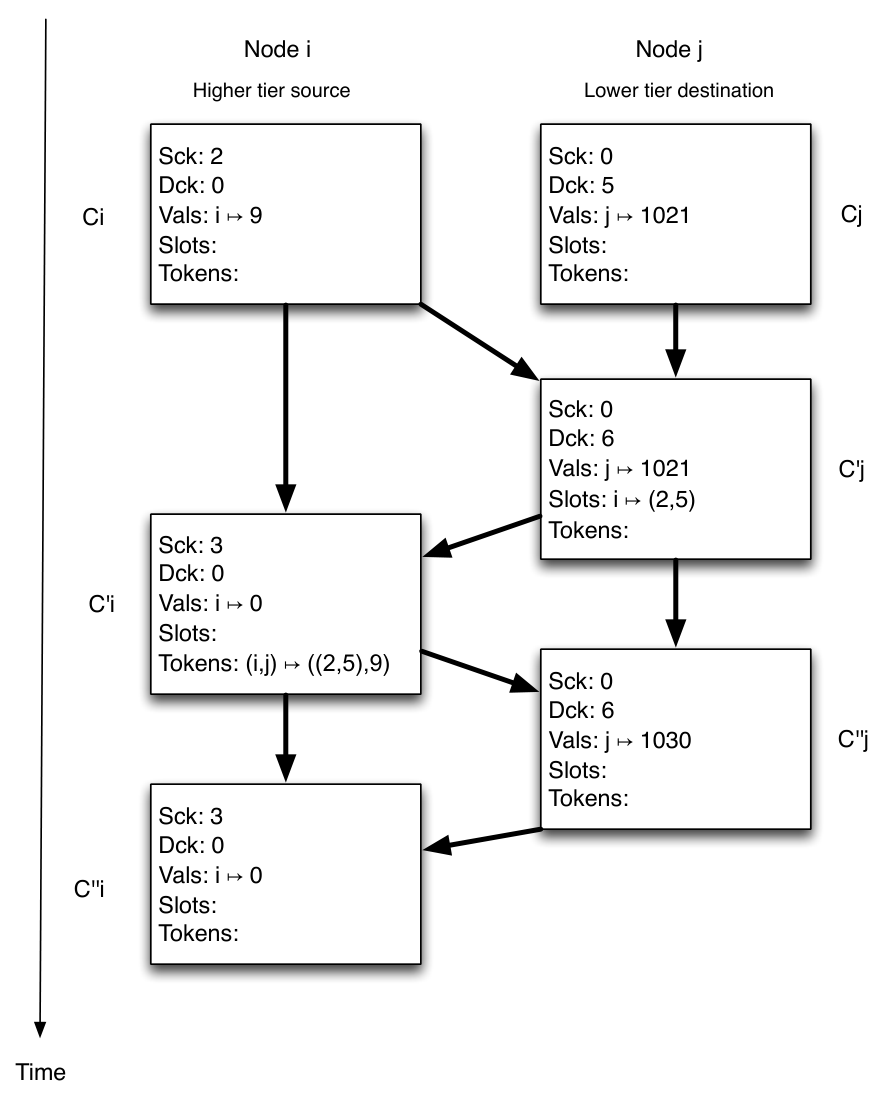
The end result of such an exchange is that an accounted value has been moved from node $i$ to node $j$ , and neither $i$ has a $j$ specific entry in its state $C^{\prime\prime}_{i}$ , nor $j$ has a $i$ specific entry in $C^{\prime\prime}_{j}$ . Temporary entries (slots and tokens) were garbage collected.

It should be noted that, although a given handoff takes 4 steps, when a pair of nodes keep exchanging messages continuously, handoffs are pipelined: steps 1 and 3 are overlapped, as well as steps 2 and 4. When a message from a node $i$ arrives at a smaller tier node $j$ , it typically carries a token, which is acquired, filling the current slot at $j$ , and a new slot is created; when the “reply” from $j$ arrives at $i$ , it makes $i$ garbage collect the current token, and a new token is created. This means that in the normal no-loss scenario, each round-trip moves an accounted value (some number of increments) from $i$ to $j$ .

The mechanism must, however, ensure correctness no matter what communication patterns may occur. Several properties are assured, namely:

•

A given slot cannot be created more than once; even if it was created, later removed and later a duplicate message arrives;
•

A token is created specifically for a given slot, and does not match any other slot;
•

A given token cannot be created more than once; even if it was created, later removed and later a duplicate message having the corresponding slot arrives.

Towards this, the CRDT keeps a pair of logical clocks, source clock and destination clock, that are used when a node plays the role of source of handoff and destination of handoff, respectively. A slot or token is identified by the quadruple: source id, destination id, source clock, destination clock. When creating a slot the destination clock is incremented; when creating a token for a given slot, the source clock is checked and incremented. This assures that neither a given slot nor a given token can be created more than once.

Figure 2 shows an execution that moves a count of 9 from node $i$ to node $j$ , illustrating the evolution, after each merge, of the subset of fields in the state that are more closely related to the handoff procedure.

The reason for two logical clocks per node (one would suffice for safety) is to allow a middle tier node to play both roles (source and destination), allowing the counter used for handoffs the node has started (as source) to remain unchanged so that the handoff may complete, even if the node is a busy server and is itself being the destination of handoffs. With a single clock there would be the danger that during the round-trip to a smaller tier node, messages from clients arrive, increasing the clock when creating a slot, and making the handoff attempt to fail (as no token would be created) and need to be repeated; under heavy load progress could be compromised.

Each handoff counter keeps a map $\mathop{\hbox{$\mathsf{vals}$}}\nolimits$ with an entry which is only incremented or added-to locally; in the case of tier 0 nodes there are also entries regarding other tier 0 nodes. In other words, each node keeps a structure similar to a version vector, mapping node ids to integers, which has only the self entry in the case of non tier 0 nodes, and also other tier 0 nodes entries in the case of tier 0 nodes.

Towards ensuring local monotonicity in reporting, while allowing values to move between nodes, each handoff counter has two integer fields, $\mathop{\hbox{$\mathsf{val}$}}\nolimits$ and $\mathop{\hbox{$\mathsf{below}$}}\nolimits$ , always updated in a non-decreasing way. Field $\mathop{\hbox{$\mathsf{val}$}}\nolimits$ keeps the maximum counter value that can be safely reported according to local knowledge. Field $\mathop{\hbox{$\mathsf{below}$}}\nolimits$ keeps a lower bound of values accounted in strictly smaller tiers; namely, it summarizes knowledge about tier 0 version vectors, avoiding the need for their dissemination to other tiers. The state of a handoff counter is then a record with the fields as in Figure 3.

$\mathop{\hbox{$\mathsf{id}$}}\nolimits$ :: node id;
$\mathop{\hbox{$\mathsf{tier}$}}\nolimits$ :: node tier;
$\mathop{\hbox{$\mathsf{val}$}}\nolimits$ :: maximum counter value that can be safely reported given local knowledge;
$\mathop{\hbox{$\mathsf{below}$}}\nolimits$ :: lower bound of values accounted in smaller tiers;
$\mathop{\hbox{$\mathsf{vals}$}}\nolimits$ :: map from ids to integers; with a single self entry if tier other than 0;
$\mathop{\hbox{$\mathsf{sck}$}}\nolimits$ :: source clock – logical clock incremented when creating tokens;
$\mathop{\hbox{$\mathsf{dck}$}}\nolimits$ :: destination clock – logical clock incremented when creating slots;
$\mathop{\hbox{$\mathsf{slots}$}}\nolimits$ :: map from source ids to pairs $(sck,dck$ ) of logical clocks;
$\mathop{\hbox{$\mathsf{tokens}$}}\nolimits$ :: map from pairs $(i,j)$ to pairs $((sck,dck),n)$ containing a pair of logical clocks and an integer;

Figure 3: Handoff Counter data type state (record fields)

The entries that keep tokens, slots and vals have been optimized, using maps as opposed to sets, namely to obtain a fast lookup in the case of slots. This is relevant as there may exist a considerable number of slots, depending on the number of concurrent clients, while there are typically very few tokens (just one in the more normal case). Such is possible due to the following:

•

Each node $j$ needs to keep at most one slot for any given node $i$ . Therefore, a slot $(i,j,sck,dck)$ is kept as an entry mapping $i$ to pairs $(sck,dck)$ in the slot map at $j$ .
•

For each pair of nodes $i$ and $j$ , there is only the need to keep at most one token of the form $((i,j,sck,dck),n)$ . However, such token may be kept at nodes other than $i$ . Tokens are stored in maps from pairs $(i,j)$ to pairs $((sck,dck),n)$ .

The Handoff Counter data type is shown in Figure 4. The $\mathop{\hbox{$\mathsf{init}$}}\nolimits$ operation creates a new CRDT instance (replica) for the counter; it takes as parameters the node id and tier number; it should be invoked only once for each globally unique id. Operation $\mathop{\hbox{$\mathsf{fetch}$}}\nolimits$ simply returns the $\mathop{\hbox{$\mathsf{val}$}}\nolimits$ field, which caches the higher counter value known so far. Operation $\mathop{\hbox{$\mathsf{incr}$}}\nolimits$ increments both the self entry in the “version vector” (i.e., $\mathop{\hbox{$\mathsf{vals}$}}\nolimits_{i}(i)$ ) and the cached value in $\mathop{\hbox{$\mathsf{val}$}}\nolimits$ . For the purposes of conciseness and clarity, in a definition of an operation $\mathop{\hbox{$\mathsf{op}$}}\nolimits(C_{i})\stackrel{{\scriptstyle.}}{{=}}\ldots$ , the fields of $C_{i}$ can be accessed in the form $\mathop{\hbox{$\mathsf{field}$}}\nolimits_{i}$ , e.g., $\mathop{\hbox{$\mathsf{tokens}$}}\nolimits_{i}$ , and $C_{i}$ denotes a record with field $\mathop{\hbox{$\mathsf{id}$}}\nolimits$ containing $i$ ; i.e., $C_{i}\stackrel{{\scriptstyle.}}{{=}}\{\mathop{\hbox{$\mathsf{id}$}}\nolimits=i,\mathop{\hbox{$\mathsf{tier}$}}\nolimits=\mathop{\hbox{$\mathsf{tier}$}}\nolimits_{i},\ldots\}$ .

$\displaystyle\mathop{\hbox{$\mathsf{init}$}}\nolimits(i,t)$	$\displaystyle\stackrel{{\scriptstyle.}}{{=}}$	$\displaystyle\{\mathop{\hbox{$\mathsf{id}$}}\nolimits=i,\mathop{\hbox{$\mathsf{tier}$}}\nolimits=t,\mathop{\hbox{$\mathsf{val}$}}\nolimits=0,\mathop{\hbox{$\mathsf{below}$}}\nolimits=0,\mathop{\hbox{$\mathsf{sck}$}}\nolimits=0,\mathop{\hbox{$\mathsf{dck}$}}\nolimits=0,$
		$\displaystyle\hphantom{\lx@text@lbrace}\mathop{\hbox{$\mathsf{slots}$}}\nolimits=\{\},\mathop{\hbox{$\mathsf{tokens}$}}\nolimits=\{\},\mathop{\hbox{$\mathsf{vals}$}}\nolimits=\{i\mapsto 0\}\}$
$\displaystyle\mathop{\hbox{$\mathsf{fetch}$}}\nolimits(C_{i})$	$\displaystyle\stackrel{{\scriptstyle.}}{{=}}$	$\displaystyle\mathop{\hbox{$\mathsf{val}$}}\nolimits_{i}$
$\displaystyle\mathop{\hbox{$\mathsf{incr}$}}\nolimits(C_{i})$	$\displaystyle\stackrel{{\scriptstyle.}}{{=}}$	$\displaystyle C_{i}\{\mathop{\hbox{$\mathsf{val}$}}\nolimits=\mathop{\hbox{$\mathsf{val}$}}\nolimits_{i}+1,\mathop{\hbox{$\mathsf{vals}$}}\nolimits=\mathop{\hbox{$\mathsf{vals}$}}\nolimits_{i}\{i\mapsto\mathop{\hbox{$\mathsf{vals}$}}\nolimits_{i}(i)+1\}\}$
$\displaystyle\mathop{\hbox{$\mathsf{merge}$}}\nolimits(C_{i},C_{j})$	$\displaystyle\stackrel{{\scriptstyle.}}{{=}}$	$\displaystyle\mathop{\hbox{$\mathsf{cachetokens}$}}\nolimits(\mathop{\hbox{$\mathsf{createtoken}$}}\nolimits(\mathop{\hbox{$\mathsf{discardtokens}$}}\nolimits(\mathop{\hbox{$\mathsf{aggregate}$}}\nolimits($
		$\displaystyle\mathop{\hbox{$\mathsf{mergevectors}$}}\nolimits(\mathop{\hbox{$\mathsf{createslot}$}}\nolimits(\mathop{\hbox{$\mathsf{discardslot}$}}\nolimits(\mathop{\hbox{$\mathsf{fillslots}$}}\nolimits(C_{i},C_{j}),C_{j}),$
		$\displaystyle C_{j}),C_{j}),C_{j}),C_{j}),C_{j}),C_{j})$

Figure 4: Handoff Counter data type operations

The CRDT $\mathop{\hbox{$\mathsf{merge}$}}\nolimits$ operation is by far the most complex one. It can be written as the composition of 8 transformations that are successively applied, each taking the result of the previous transformation and the received instance as parameters. Each of these transformations takes care of a different aspect of merging the two instances into a new one; they are presented in Figure 5, where the following notation is used.

Notation

We use mostly standard notation for sets and maps/relations. A map is a set of $(k,v)$ pairs (a relation), where each $k$ is associated with a single $v$ ; to emphasize the functional relationship we also use $k\mapsto v$ for entries in a map. We use $M\{\ldots\}$ for map update; $M\{x\mapsto 3\}$ maps $x$ to $3$ and behaves like $M$ otherwise. For records we use similar notations but with $=$ instead of $\mapsto$ , to emphasize a fixed set of keys. We use $\mathop{\lhd\mkern-14.0mu-}$ for domain subtraction; $S\mathop{\lhd\mkern-14.0mu-}M$ is the map obtained by removing from $M$ all pairs $(k,v)$ with $k\in S$ . We use set comprehension of the forms $\{x\in S|P(x)\}$ or $\{f(x)|x\in S|P(x)\}$ , or list comprehensions, using square brackets instead. The domain of a relation $R$ is denoted by $\mathop{\hbox{$\mathsf{dom}$}}\nolimits(R)$ , while $\mathop{\hbox{$\mathsf{fst}$}}\nolimits(T)$ and $\mathop{\hbox{$\mathsf{snd}$}}\nolimits(T)$ denote the first and second component, respectively, of a tuple $T$ . We use $\cup^{f}(m,m^{\prime})$ to represent joining maps while applying $f$ to the values corresponding to common keys, i.e., $\cup^{f}(m,m^{\prime})=\{(k,v)\in m|k\notin\mathop{\hbox{$\mathsf{dom}$}}\nolimits(m^{\prime})\}\cup\{(k,v)\in m^{\prime}|k\notin\mathop{\hbox{$\mathsf{dom}$}}\nolimits(m)\}\cup\{(k,f(m(k),m^{\prime}(k)))|k\in\mathop{\hbox{$\mathsf{dom}$}}\nolimits(m)\cap\mathop{\hbox{$\mathsf{dom}$}}\nolimits(m^{\prime})\}$ . To define a function or predicate by cases, we use $\mathrel{\hbox{$\mathbf{if}$}}X\mathrel{\hbox{$\mathbf{then}$}} Y\mathrel{\hbox{$\mathbf{else}$}} Z$ to mean “ $Y$ if $X$ is true, $Z$ otherwise”.

$\displaystyle\mathop{\hbox{$\mathsf{fillslots}$}}\nolimits(C_{i},C_{j})$	$\displaystyle\stackrel{{\scriptstyle.}}{{=}}$	$\displaystyle C_{i}\{\mathop{\hbox{$\mathsf{vals}$}}\nolimits=\mathop{\hbox{$\mathsf{vals}$}}\nolimits_{i}\{i\mapsto\mathop{\hbox{$\mathsf{vals}$}}\nolimits_{i}(i)+\sum[n\|(\_,n)\in S]\},$
		$\displaystyle\hphantom{C_i\lx@text@lbrace}\mathop{\hbox{$\mathsf{slots}$}}\nolimits=\mathop{\hbox{$\mathsf{dom}$}}\nolimits(S)\mathop{\lhd\mkern-14.0mu-}\mathop{\hbox{$\mathsf{slots}$}}\nolimits_{i}\}$
		$\displaystyle\mathrel{\hbox{$\mathbf{where}$}}S\stackrel{{\scriptstyle.}}{{=}}\{(src,n)\|((src,dst),(ck,n))\in\mathop{\hbox{$\mathsf{tokens}$}}\nolimits_{j}\|$
		$\displaystyle\hphantom{\mathrel{\hbox{$\mathbf{where}$}} S \stackrel{{\scriptstyle.}}{{=}}\lx@text@lbrace (src, n) \| {}}dst=i\mathrel{\wedge}(src,ck)\in\mathop{\hbox{$\mathsf{slots}$}}\nolimits_{i}\}$
$\displaystyle\mathop{\hbox{$\mathsf{discardslot}$}}\nolimits(C_{i},C_{j})$	$\displaystyle\stackrel{{\scriptstyle.}}{{=}}$	$\displaystyle\mathrel{\hbox{$\mathbf{if}$}}j\in\mathop{\hbox{$\mathsf{dom}$}}\nolimits(\mathop{\hbox{$\mathsf{slots}$}}\nolimits_{i})\mathrel{\wedge}\mathop{\hbox{$\mathsf{sck}$}}\nolimits_{j}>\mathop{\hbox{$\mathsf{fst}$}}\nolimits(\mathop{\hbox{$\mathsf{slots}$}}\nolimits_{i}(j))$
		$\displaystyle\mathrel{\hbox{$\mathbf{then}$}}C_{i}\{\mathop{\hbox{$\mathsf{slots}$}}\nolimits=\{j\}\mathop{\lhd\mkern-14.0mu-}\mathop{\hbox{$\mathsf{slots}$}}\nolimits_{i}\}$
		$\displaystyle\mathrel{\hbox{$\mathbf{else}$}}C_{i}$
$\displaystyle\mathop{\hbox{$\mathsf{createslot}$}}\nolimits(C_{i},C_{j})$	$\displaystyle\stackrel{{\scriptstyle.}}{{=}}$	$\displaystyle\mathrel{\hbox{$\mathbf{if}$}}\mathop{\hbox{$\mathsf{tier}$}}\nolimits_{i}<\mathop{\hbox{$\mathsf{tier}$}}\nolimits_{j}\mathrel{\wedge}\mathop{\hbox{$\mathsf{vals}$}}\nolimits_{j}(j)>0\mathrel{\wedge}j\notin\mathop{\hbox{$\mathsf{dom}$}}\nolimits(\mathop{\hbox{$\mathsf{slots}$}}\nolimits_{i})$
		$\displaystyle\mathrel{\hbox{$\mathbf{then}$}}C_{i}\{\mathop{\hbox{$\mathsf{slots}$}}\nolimits=\mathop{\hbox{$\mathsf{slots}$}}\nolimits_{i}\{j\mapsto(\mathop{\hbox{$\mathsf{sck}$}}\nolimits_{j},\mathop{\hbox{$\mathsf{dck}$}}\nolimits_{i})\},\mathop{\hbox{$\mathsf{dck}$}}\nolimits=\mathop{\hbox{$\mathsf{dck}$}}\nolimits_{i}+1\}$
		$\displaystyle\mathrel{\hbox{$\mathbf{else}$}}C_{i}$
$\displaystyle\mathop{\hbox{$\mathsf{mergevectors}$}}\nolimits(C_{i},C_{j})$	$\displaystyle\stackrel{{\scriptstyle.}}{{=}}$	$\displaystyle\begin{array}[t]{@{}l@{\ }l}\mathrel{\hbox{$\mathbf{if}$}}\mathop{\hbox{$\mathsf{tier}$}}\nolimits_{i}=\mathop{\hbox{$\mathsf{tier}$}}\nolimits_{j}=0&\mathrel{\hbox{$\mathbf{then}$}}C_{i}\{\mathop{\hbox{$\mathsf{vals}$}}\nolimits=\cup^{\max}(\mathop{\hbox{$\mathsf{vals}$}}\nolimits_{i},\mathop{\hbox{$\mathsf{vals}$}}\nolimits_{j})\}\\ &\mathrel{\hbox{$\mathbf{else}$}}C_{i}\end{array}$
$\displaystyle\mathop{\hbox{$\mathsf{aggregate}$}}\nolimits(C_{i},C_{j})$	$\displaystyle\stackrel{{\scriptstyle.}}{{=}}$	$\displaystyle C_{i}\{\mathop{\hbox{$\mathsf{below}$}}\nolimits=b,\mathop{\hbox{$\mathsf{val}$}}\nolimits=v\}$
		$\displaystyle\mathrel{\hbox{$\mathbf{where}$}}b\stackrel{{\scriptstyle.}}{{=}}\begin{array}[t]{@{}l}\mathrel{\hbox{$\mathbf{if}$}}\mathop{\hbox{$\mathsf{tier}$}}\nolimits_{i}=\mathop{\hbox{$\mathsf{tier}$}}\nolimits_{j}\mathrel{\hbox{$\mathbf{then}$}}\max(\mathop{\hbox{$\mathsf{below}$}}\nolimits_{i},\mathop{\hbox{$\mathsf{below}$}}\nolimits_{j})\\ \mathrel{\hbox{$\mathbf{else}$}}\ \mathrel{\hbox{$\mathbf{if}$}}\mathop{\hbox{$\mathsf{tier}$}}\nolimits_{i}>\mathop{\hbox{$\mathsf{tier}$}}\nolimits_{j}\mathrel{\hbox{$\mathbf{then}$}}\max(\mathop{\hbox{$\mathsf{below}$}}\nolimits_{i},\mathop{\hbox{$\mathsf{val}$}}\nolimits_{j})\\ \mathrel{\hbox{$\mathbf{else}$}}\mathop{\hbox{$\mathsf{below}$}}\nolimits_{i}\end{array}$
		$\displaystyle\hphantom{\mathrel{\hbox{$\mathbf{where}$}}{}}v\stackrel{{\scriptstyle.}}{{=}}\begin{array}[t]{@{}l}\mathrel{\hbox{$\mathbf{if}$}}\mathop{\hbox{$\mathsf{tier}$}}\nolimits_{i}=0\mathrel{\hbox{$\mathbf{then}$}}\sum[n\|(\_,n)\in\mathop{\hbox{$\mathsf{vals}$}}\nolimits_{i}]\\ \mathrel{\hbox{$\mathbf{else}$}}\ \mathrel{\hbox{$\mathbf{if}$}}\mathop{\hbox{$\mathsf{tier}$}}\nolimits_{i}=\mathop{\hbox{$\mathsf{tier}$}}\nolimits_{j}\mathrel{\hbox{$\mathbf{then}$}}\max(\mathop{\hbox{$\mathsf{val}$}}\nolimits_{i},\mathop{\hbox{$\mathsf{val}$}}\nolimits_{j},b+\mathop{\hbox{$\mathsf{vals}$}}\nolimits_{i}(i)+\mathop{\hbox{$\mathsf{vals}$}}\nolimits_{j}(j))\\ \mathrel{\hbox{$\mathbf{else}$}}\max(\mathop{\hbox{$\mathsf{val}$}}\nolimits_{i},b+\mathop{\hbox{$\mathsf{vals}$}}\nolimits_{i}(i))\end{array}$
$\displaystyle\mathop{\hbox{$\mathsf{discardtokens}$}}\nolimits(C_{i},C_{j})$	$\displaystyle\stackrel{{\scriptstyle.}}{{=}}$	$\displaystyle C_{i}\{\mathop{\hbox{$\mathsf{tokens}$}}\nolimits=\{(k,v)\in\mathop{\hbox{$\mathsf{tokens}$}}\nolimits_{i}\|\neg P(k,v)\}$
		$\displaystyle\mathrel{\hbox{$\mathbf{where}$}}P((src,dst),((\_,dck),\_))\stackrel{{\scriptstyle.}}{{=}}(dst=j)\mathrel{\wedge}$
		$\displaystyle\qquad\qquad\begin{array}[]{l@{\ }l}\mathrel{\hbox{$\mathbf{if}$}}src\in\mathop{\hbox{$\mathsf{dom}$}}\nolimits(\mathop{\hbox{$\mathsf{slots}$}}\nolimits_{j})&\mathrel{\hbox{$\mathbf{then}$}}\mathop{\hbox{$\mathsf{snd}$}}\nolimits(\mathop{\hbox{$\mathsf{slots}$}}\nolimits_{j}(src))>dck\\ &\mathrel{\hbox{$\mathbf{else}$}}\mathop{\hbox{$\mathsf{dck}$}}\nolimits_{j}>dck\end{array}$
$\displaystyle\mathop{\hbox{$\mathsf{createtoken}$}}\nolimits(C_{i},C_{j})$	$\displaystyle\stackrel{{\scriptstyle.}}{{=}}$	$\displaystyle\mathrel{\hbox{$\mathbf{if}$}}i\in\mathop{\hbox{$\mathsf{dom}$}}\nolimits(\mathop{\hbox{$\mathsf{slots}$}}\nolimits_{j})\mathrel{\wedge}\mathop{\hbox{$\mathsf{fst}$}}\nolimits(\mathop{\hbox{$\mathsf{slots}$}}\nolimits_{j}(i))=\mathop{\hbox{$\mathsf{sck}$}}\nolimits_{i}$
		$\displaystyle\mathrel{\hbox{$\mathbf{then}$}}\begin{array}[t]{@{}l@{}l}C_{i}\{&\mathop{\hbox{$\mathsf{tokens}$}}\nolimits=\mathop{\hbox{$\mathsf{tokens}$}}\nolimits_{i}\{(i,j)\mapsto(\mathop{\hbox{$\mathsf{slots}$}}\nolimits_{j}(i),\mathop{\hbox{$\mathsf{vals}$}}\nolimits_{i}(i))\},\\ &\mathop{\hbox{$\mathsf{vals}$}}\nolimits=\mathop{\hbox{$\mathsf{vals}$}}\nolimits_{i}\{i\mapsto 0\},\\ &\mathop{\hbox{$\mathsf{sck}$}}\nolimits=\mathop{\hbox{$\mathsf{sck}$}}\nolimits_{i}+1\}\end{array}$
		$\displaystyle\mathrel{\hbox{$\mathbf{else}$}}C_{i}$
$\displaystyle\mathop{\hbox{$\mathsf{cachetokens}$}}\nolimits(C_{i},C_{j})$	$\displaystyle\stackrel{{\scriptstyle.}}{{=}}$	$\displaystyle\mathrel{\hbox{$\mathbf{if}$}}\mathop{\hbox{$\mathsf{tier}$}}\nolimits_{i}<\mathop{\hbox{$\mathsf{tier}$}}\nolimits_{j}$
		$\displaystyle\mathrel{\hbox{$\mathbf{then}$}}C_{i}\{\mathop{\hbox{$\mathsf{tokens}$}}\nolimits=\cup^{f}(\mathop{\hbox{$\mathsf{tokens}$}}\nolimits_{i},t)\}$
		$\displaystyle\hphantom{\mathrel{\hbox{$\mathbf{then}$}}}\mathrel{\hbox{$\mathbf{where}$}}t\stackrel{{\scriptstyle.}}{{=}}\{((src,dst),v)\in\mathop{\hbox{$\mathsf{tokens}$}}\nolimits_{j}\|src=j\mathrel{\wedge}dst\neq i\},$
		$\displaystyle\hphantom{\mathrel{\hbox{$\mathbf{then}$}}\mathrel{\hbox{$\mathbf{where}$}}{}}f((ck,n),(ck^{\prime},n^{\prime}))\stackrel{{\scriptstyle.}}{{=}}\begin{array}[t]{l@{\ }l}\mathrel{\hbox{$\mathbf{if}$}}\mathop{\hbox{$\mathsf{fst}$}}\nolimits(ck)\geq\mathop{\hbox{$\mathsf{fst}$}}\nolimits(ck^{\prime})&\mathrel{\hbox{$\mathbf{then}$}}(ck,n)\\ &\mathrel{\hbox{$\mathbf{else}$}}(ck^{\prime},n^{\prime})\end{array}$
		$\displaystyle\mathrel{\hbox{$\mathbf{else}$}}C_{i}$

Figure 5: Handoff Counter auxiliary transformations in

\mathop{\hbox{$\mathsf{merge}$}}\nolimits

We now describe informally each of these transformations used in $\mathop{\hbox{$\mathsf{merge}$}}\nolimits$ . We leave the formal proof of correctness for the next section.

$\mathop{\hbox{$\mathsf{fillslots}$}}\nolimits(C_{i},C_{j})$

Fills all possible slots in $C_{i}$ for which there are matching tokens in $C_{j}$ , removing them from $\mathop{\hbox{$\mathsf{slots}$}}\nolimits_{i}$ and adding the counter values in the tokens to the self version vector entry $\mathop{\hbox{$\mathsf{vals}$}}\nolimits_{i}(i)$ . We call this transfer of a counter value in a token to the $\mathop{\hbox{$\mathsf{vals}$}}\nolimits$ entry of the destination node acquiring the token and the corresponding slot removal filling the slot.

$\mathop{\hbox{$\mathsf{discardslot}$}}\nolimits(C_{i},C_{j})$

Discards a slot, if any, in $C_{i}$ for source $j$ , that cannot ever be possibly filled by a matching token, because $C_{j}$ assures no such token will ever be generated. For such a slot that still remains in $C_{i}$ (and, therefore, has not been filled by a matching token in $C_{j}$ by the just applied $\mathop{\hbox{$\mathsf{fillslots}$}}\nolimits$ ) this is the case if the source clock at $C_{j}$ is greater than the corresponding value in the slot.

$\mathop{\hbox{$\mathsf{createslot}$}}\nolimits(C_{i},C_{j})$

Creates a slot in $C_{i}$ for a higher tier source node $j$ , if $C_{j}$ has some non-zero value to handoff and there is no slot for $j$ at $C_{i}$ . If a slot is created, the local destination clock is stored in it and increased, preventing duplicate creation of the same slot in case of duplicate messages. A slot merely opens the possibility of node $j$ creating a corresponding token; not all slots will have corresponding tokens, some will be discarded or replaced by newer slots. In fact, the local knowledge in $C_{i}$ after discarding $j$ specific information makes it impossible to avoid creating a slot upon a slow or duplicate message; this is not a problem as such slots will never match any token, being eventually discarded upon further communication.

$\mathop{\hbox{$\mathsf{mergevectors}$}}\nolimits(C_{i},C_{j})$

Merges the corresponding version vector entries, doing a pointwise maximum for common ids. This is only done when merging two tier 0 replicas.

$\mathop{\hbox{$\mathsf{aggregate}$}}\nolimits(C_{i},C_{j})$

Performs a vertical aggregation step (from smaller to higher tiers up to the current one), that updates the $\mathop{\hbox{$\mathsf{below}$}}\nolimits$ and $\mathop{\hbox{$\mathsf{val}$}}\nolimits$ fields according to the knowledge provided by $C_{j}$ . This can never decrease their current values. The effect is to propagate values accounted in tier 0 version vectors, while adding knowledge provided by intermediate nodes, up to $C_{i}$ and $C_{j}$ .

$\mathop{\hbox{$\mathsf{discardtokens}$}}\nolimits(C_{i},C_{j})$

Discards from $C_{i}$ the tokens that have already been acquired by $C_{j}$ ; this is the case for tokens with id $(src,j,\_,dck)$ if either there is a slot $(src,j,\_,dck^{\prime})$ at $C_{j}$ with $dck^{\prime}>dck$ or if there is no slot $(src,j,\_,\_)$ at $C_{j}$ and $\mathop{\hbox{$\mathsf{dck}$}}\nolimits_{j}>dck$ . Here $src$ is normally, but not necessarily, equal to $i$ , as $C_{i}$ can cache tokens from another source than $i$ .

$\mathop{\hbox{$\mathsf{createtoken}$}}\nolimits(C_{i},C_{j})$

Creates a token, to which the currently accounted value in $\mathop{\hbox{$\mathsf{vals}$}}\nolimits_{i}(i)$ is moved, if there is a slot for $i$ in $C_{j}$ having a source clock equal to the current one at $C_{i}$ . If a token is created, the local source clock is increased, preventing duplicate creation of the same token in case of duplicate messages.

$\mathop{\hbox{$\mathsf{cachetokens}$}}\nolimits(C_{i},C_{j})$

Keeps a copy of tokens generated at a higher tier node $j$ meant to some other destination $k$ . For each pair source-destination, older tokens (that must have already been acquired) are replaced by newer ones. Caching tokens provides availability under faults, as it allows a client $j$ in the middle of a handoff to $k$ , to delegate to $i$ the responsibility of finishing the handoff, in case $j$ wants to terminate but either $k$ has crashed and is recovering or the link between $j$ and $k$ is currently down. Only tokens that have been generated at node $j$ are cached (other tokens currently cached at $j$ are not considered) so that alternate handoff routes are provided, while preventing the flooding and the large sets of tokens that would result from a transitive dissemination of tokens to other nodes.

5.4 Implementation and Experimental Validation

The development of Handoff Counters was made in tandem with a prototype implementation and checked by a testing infrastructure that allows for randomized runs over given topologies. These runs exercised the solution robustness, in particular by replaying old messages out of order, and allowed to detect and correct several corner cases, enabling the correction of subtle bugs that existed in tentative versions of the mechanism.

Although testing does not ensure correctness, the current implementation has successfully passed randomized traces with up to one hundred million steps, both in giving the correct result and also in garbage collecting temporary entries, making it a complement to a manual formal proof (which is prone to human errors).

An experimentally robust solution was thus a prelude to the formal correctness proof in the following section, and added an independent assessment to the overall approach. The implementation and testing infrastructure, written in Clojure, is publicly available in GitHub (https://github.com/pssalmeida/clj-crdt), and serves as a complement to this article.

6 Correctness

Lemma 6.1.

Any slot $(s,d,sck,dck)$ can be created at most once.

Proof.

Each node uses its own id as $d$ in the slot; therefore, no two nodes can create the same slot. In each node, a slot is only created when applying $\mathop{\hbox{$\mathsf{createslot}$}}\nolimits$ , which also increments $\mathop{\hbox{$\mathsf{dck}$}}\nolimits$ upon storing it in the slot; therefore, a subsequent $\mathop{\hbox{$\mathsf{createslot}$}}\nolimits$ in the same node cannot create the same slot. ∎

Lemma 6.2.

Any token with id $(s,d,sck,dck)$ can be created at most once.

Proof.

Each node uses its own id as $s$ when creating the token; therefore, no two nodes can create the same token. In each node $\mathop{\hbox{$\mathsf{createtoken}$}}\nolimits$ also increments $\mathop{\hbox{$\mathsf{sck}$}}\nolimits$ upon storing it in the token; therefore, a subsequent $\mathop{\hbox{$\mathsf{createtoken}$}}\nolimits$ in the same node cannot create the same token. ∎

Lemma 6.3.

Any token with id $(s,d,sck,dck)$ can be acquired at most once.

Proof.

Such token can only be acquired in node $d$ having a corresponding slot $(s,d,sck,dck)$ while performing the $\mathop{\hbox{$\mathsf{fillslots}$}}\nolimits$ function, which removes this slot from the resulting state, preventing a subsequent acquisition of the same token, as due to Lemma 6.1 this slot cannot be recreated. ∎

Proposition 6.1.

Given a token $T$ with id $(s,d,sck,dck)$ : (i) $T$ will not be removed from any node before it has been acquired; (ii) a corresponding slot $S$ will exist in node $d$ between the time when $T$ is created and the time when $T$ is acquired.

Proof.

By induction on the trace of the actions performed by the system, using (i) and (ii) together in the induction hypothesis. The only relevant action is $\mathop{\hbox{$\mathsf{receive}$}}\nolimits_{j,i}(C_{j})$ of a message previously sent by a node $j$ to a node $i$ , with the corresponding merge being applied to the state of $i$ . Given the asynchronous system model allowing message duplicates, we must assume that $C_{j}$ can be the state of $j$ at any point in the past, due to some $\mathop{\hbox{$\mathsf{send}$}}\nolimits_{j,i}$ action that resulted in a message arbitrarily delayed and/or duplicated.

Regarding (i), a token $T$ with id $(s,d,sck,dck)$ can only be removed either: (1) In $\mathop{\hbox{$\mathsf{discardtokens}$}}\nolimits$ when merging with a state $C$ from $d$ , having either a slot $(s,d,\_,dck^{\prime})$ with $dck^{\prime}>dck$ , or with no slot for $s$ and the destination clock in $C$ greater than $dck$ ; either way, given that slots for destination $d$ are created with increasing destination clock values, it implies that $C$ corresponds to a time after slot $S$ was created. By the induction hypothesis, $S$ would have existed until $T$ was acquired, and as $S$ is absent from $C$ , this implies that $T$ was already acquired. (2) Or $T$ could be removed by the $\mathop{\hbox{$\mathsf{tokens}$}}\nolimits$ map entry for $(s,d)$ being overwritten in $\mathop{\hbox{$\mathsf{createtoken}$}}\nolimits$ ; this last case is not possible because: tokens are created using the current source clock, which is then incremented; for a token with id $(s,d,\mathop{\hbox{$\mathsf{sck}$}}\nolimits_{s},\_)$ to be created, a received counter state $C$ from $d$ must contain a slot $(s,d,sck^{\prime},\_)$ with $sck^{\prime}=\mathop{\hbox{$\mathsf{sck}$}}\nolimits_{s}$ . This means that $d$ would have previously received $T$ from $s$ and from the induction hypothesis, $d$ would have had a corresponding slot and would have already acquired $T$ filling the slot. When $C$ arrived at $s$ , $T$ would be discarded by $\mathop{\hbox{$\mathsf{discardtokens}$}}\nolimits$ before invoking $\mathop{\hbox{$\mathsf{createtoken}$}}\nolimits$ , i.e., as in the first case above.

Regarding (ii), $T$ is created, in $\mathop{\hbox{$\mathsf{createtoken}$}}\nolimits$ , only if a corresponding slot has been created at some previous time in node $d$ ; this slot can only be removed either: in $\mathop{\hbox{$\mathsf{fillslots}$}}\nolimits$ , when $T$ is acquired; or in $\mathop{\hbox{$\mathsf{discardslot}$}}\nolimits$ , when merging with a counter $C$ from node $s$ whose source clock is greater than $sck$ , implying a state in $s$ after $T$ has been created. But in this case this slot at node $d$ cannot reach the $\mathop{\hbox{$\mathsf{discardslot}$}}\nolimits$ function as, by the induction hypothesis, $T$ would be present in $C$ and would have been acquired by $\mathop{\hbox{$\mathsf{fillslots}$}}\nolimits$ , filling the slot, just before invoking $\mathop{\hbox{$\mathsf{discardslot}$}}\nolimits$ . ∎

Lemma 6.4.

Any token with id $(s,d,sck,dck)$ will be eventually acquired.

Proof.

Such token, created at node $s$ , must have resulted from direct message exchanges between $s$ and a smaller tier node $d$ . From Proposition 6.1, this token will remain at $s$ and a corresponding slot will exist at $d$ until the token is acquired. As $s$ will keep sending its $C_{s}$ to its neighbors, therefore to $d$ , and from the system model assumptions (Section 3.1) messages eventually get through, if the token has not yet been acquired (e.g., by communication between $d$ and some other node caching the token), $C_{s}$ containing the token will eventually arrive at $d$ , which will acquire it. ∎

Definition 6.1 (Enabled token).

A token $((s,d,sck,dck),n)$ is called enabled if there exists a corresponding slot $(s,d,sck,dck)$ at node $d$ . The set of enabled tokens in a configuration (set of replicas) $C$ is denoted $E_{C}$ .

Whether a token is enabled is a global property, not decidable by nodes holding the token with local information. From Proposition 6.1, a token $T$ is enabled when created; it remains enabled until it is acquired, when the corresponding slot is filled. We also remark that $E_{C}$ is the set (as opposed to multiset) of enabled tokens; the presence of duplicates of some token $T$ created at one node and cached at some other node(s) is irrelevant.

Lemma 6.5.

Fields $\mathop{\hbox{$\mathsf{below}$}}\nolimits$ and $\mathop{\hbox{$\mathsf{val}$}}\nolimits$ are non-decreasing.

Proof.

By induction on the trace of the actions performed by the system. These fields only change by an $\mathop{\hbox{$\mathsf{incr}$}}\nolimits_{i}$ at node $i$ , which increments $\mathop{\hbox{$\mathsf{val}$}}\nolimits_{i}$ , or when doing a merge when receiving a message, in $\mathop{\hbox{$\mathsf{aggregate}$}}\nolimits$ , which either updates $\mathop{\hbox{$\mathsf{below}$}}\nolimits$ and $\mathop{\hbox{$\mathsf{val}$}}\nolimits$ using a maximum involving the respective current value, or stores in $\mathop{\hbox{$\mathsf{val}$}}\nolimits_{i}$ the sum of $\mathop{\hbox{$\mathsf{vals}$}}\nolimits_{i}$ entries, if $i$ is a tier 0 node, which is also non-decreasing, as $\mathop{\hbox{$\mathsf{vals}$}}\nolimits_{i}$ for tier 0 nodes contain a set of entries always from tier 0 nodes, only updated by a pointwise maximum (as tier 0 nodes never create tokens). ∎

Definition 6.2 (Cumulative Tier Value).

In a configuration $C$ , the cumulative tier value for tier $k$ , written $\mathop{\hbox{$\mathsf{CTV}$}}\nolimits_{C}(k)$ , is the sum, for all nodes with tier up to $k$ , of the self component of the $\mathop{\hbox{$\mathsf{vals}$}}\nolimits$ field plus the tokens created by these nodes that are still enabled, i.e.:

	$\displaystyle\mathop{\hbox{$\mathsf{CTV}$}}\nolimits_{C}(k)$	$\displaystyle\stackrel{{\scriptstyle.}}{{=}}$	$\displaystyle\sum[\mathop{\hbox{$\mathsf{vals}$}}\nolimits_{i}(i)\|C_{i}\in C\|\mathop{\hbox{$\mathsf{tier}$}}\nolimits_{i}\leq k]+{}$
			$\displaystyle\sum[n\|((i,\_,\_,\_),n)\in E_{C}\|\mathop{\hbox{$\mathsf{tier}$}}\nolimits_{i}\leq k].$

Lemma 6.6.

For each $k$ , $\mathop{\hbox{$\mathsf{CTV}$}}\nolimits_{C}(k)$ is non-decreasing, i.e., for any transition between configurations $C$ and $C^{\prime}$ , $\mathop{\hbox{$\mathsf{CTV}$}}\nolimits_{C}(k)\leq\mathop{\hbox{$\mathsf{CTV}$}}\nolimits_{C^{\prime}}(k)$ .

Proof.

For any node $i$ , the only time $\mathop{\hbox{$\mathsf{vals}$}}\nolimits_{i}(i)$ can decrease is when a token is created, enabled, and the value is moved to the token; in this case $\mathop{\hbox{$\mathsf{CTV}$}}\nolimits_{C^{\prime}}(k)$ remains unchanged for all $k$ . When a token holding value $n$ ceases to be enabled (being acquired), $n$ is added to the $\mathop{\hbox{$\mathsf{vals}$}}\nolimits_{j}(j)$ field for some smaller tier node $j$ ; this makes $\mathop{\hbox{$\mathsf{CTV}$}}\nolimits_{C^{\prime}}(k)$ either unchanged or greater. ∎

Lemma 6.7.

$\mathop{\hbox{$\mathsf{CTV}$}}\nolimits_{C}(k)$ is monotonic over $k$ , i.e., $k_{1}\leq k_{2}\Rightarrow\mathop{\hbox{$\mathsf{CTV}$}}\nolimits_{C}(k_{1})\leq\mathop{\hbox{$\mathsf{CTV}$}}\nolimits_{C}(k_{2})$ .

Proof.

Trivial from the $\mathop{\hbox{$\mathsf{CTV}$}}\nolimits$ definition. ∎

Proposition 6.2.

For any counter replica $C_{i}$ in a configuration $C$ : (i) $\mathop{\hbox{$\mathsf{below}$}}\nolimits_{i}\leq\mathop{\hbox{$\mathsf{CTV}$}}\nolimits_{C}(\mathop{\hbox{$\mathsf{tier}$}}\nolimits_{i}-1)$ ; (ii) $\mathop{\hbox{$\mathsf{val}$}}\nolimits_{i}\leq\mathop{\hbox{$\mathsf{CTV}$}}\nolimits_{C}(\mathop{\hbox{$\mathsf{tier}$}}\nolimits_{i})$ .

Proof.

By induction on the trace of the actions performed by the system, using (i) and (ii) together in the induction hypothesis. Given that $\mathop{\hbox{$\mathsf{CTV}$}}\nolimits_{C}(k)$ is non-decreasing (by Lemma 6.6), so are the right-hand sides of the inequalities, and the only relevant actions are those that update either $\mathop{\hbox{$\mathsf{below}$}}\nolimits_{i}$ or $\mathop{\hbox{$\mathsf{val}$}}\nolimits_{i}$ : (1) An increment $\mathop{\hbox{$\mathsf{incr}$}}\nolimits_{i}$ at node $i$ , resulting in an increment of both $\mathop{\hbox{$\mathsf{val}$}}\nolimits_{i}$ and $\mathop{\hbox{$\mathsf{vals}$}}\nolimits_{i}(i)$ , in which case the inequality remains true. (2) A $\mathop{\hbox{$\mathsf{receive}$}}\nolimits_{j,i}(M)$ of a message previously sent by a node $j$ to node $i$ , with the corresponding merge being applied to the state of $i$ , and the fields being updated by $\mathop{\hbox{$\mathsf{aggregate}$}}\nolimits$ . Regarding $\mathop{\hbox{$\mathsf{below}$}}\nolimits_{i}$ , there are three cases: it remains unchanged, it can be possibly set to $\mathop{\hbox{$\mathsf{below}$}}\nolimits_{j}$ if $\mathop{\hbox{$\mathsf{tier}$}}\nolimits_{j}=\mathop{\hbox{$\mathsf{tier}$}}\nolimits_{i}$ , or it can be possibly set to $\mathop{\hbox{$\mathsf{val}$}}\nolimits_{j}$ if $\mathop{\hbox{$\mathsf{tier}$}}\nolimits_{j}<\mathop{\hbox{$\mathsf{tier}$}}\nolimits_{i}$ ; in each case the induction hypothesis is preserved because $\mathop{\hbox{$\mathsf{CTV}$}}\nolimits_{C}$ is non-decreasing ( $M$ can be any message from node $j$ , arbitrarily from the past) and in the last case also due to the monotonicity of $\mathop{\hbox{$\mathsf{CTV}$}}\nolimits_{C}(k)$ over $k$ (by Lemma 6.7). Regarding $\mathop{\hbox{$\mathsf{val}$}}\nolimits_{i}$ , either it is set to the sum of the $\mathop{\hbox{$\mathsf{vals}$}}\nolimits_{i}$ values, if $\mathop{\hbox{$\mathsf{tier}$}}\nolimits_{i}=0$ , which does not exceed $\mathop{\hbox{$\mathsf{CTV}$}}\nolimits_{C}(0)$ due to the pointwise maximum updating of $\mathop{\hbox{$\mathsf{vals}$}}\nolimits$ fields for tier 0 nodes; or it either remains unchanged, is set to $\mathop{\hbox{$\mathsf{val}$}}\nolimits_{j}$ only if $\mathop{\hbox{$\mathsf{tier}$}}\nolimits_{i}=\mathop{\hbox{$\mathsf{tier}$}}\nolimits_{j}$ , or is set to the sum of the values (computed for the next configuration) of $\mathop{\hbox{$\mathsf{below}$}}\nolimits_{i}$ with $\mathop{\hbox{$\mathsf{vals}$}}\nolimits_{i}(i)$ and also $\mathop{\hbox{$\mathsf{vals}$}}\nolimits_{j}(j)$ when $\mathop{\hbox{$\mathsf{tier}$}}\nolimits_{i}=\mathop{\hbox{$\mathsf{tier}$}}\nolimits_{j}$ ; in each case the induction hypothesis is preserved. ∎

Proposition 6.3.

The number of increments globally issued up to any time $t$ , say $I^{t}$ , is equal to the sum of the values held in the set of enabled tokens and of the self entries in the $\mathop{\hbox{$\mathsf{vals}$}}\nolimits$ field of all nodes; i.e., for a network having maximum tier $T$ , given a configuration $C^{t}$ at time $t$ , we have $I^{t}=\mathop{\hbox{$\mathsf{CTV}$}}\nolimits_{C^{t}}(T)$ .

Proof.

By induction on the trace of the actions performed by the system. The relevant actions are an increment at some node $i$ , which results in an increment of the $i$ component of the $\mathop{\hbox{$\mathsf{vals}$}}\nolimits$ field of node $i$ ; or a $\mathop{\hbox{$\mathsf{receive}$}}\nolimits_{j,i}(C_{j})$ of a message previously sent by a node $j$ to a node $i$ , with the corresponding merge being applied to the state of $i$ , leading possibly to: the filling of one or more slots, each slot $S$ corresponding to a token $(S,n)$ , which adds $n$ to $\mathop{\hbox{$\mathsf{vals}$}}\nolimits_{i}(i)$ and removes slot $S$ from $i$ , which makes the token no longer enabled, leaving the sum unchanged; discarding a slot, which cannot, however, correspond to an enabled token, as from Proposition 6.1 a slot will exist until the corresponding token is acquired; merging $\mathop{\hbox{$\mathsf{vals}$}}\nolimits$ pointwise for two tier 0 nodes, which does not change the self component $vals_{i}(i)$ of any node $i$ ; discarding tokens, which cannot be enabled because, by Proposition 6.1, tokens are only removed from any node after being acquired; the creation of an enabled token $(\_,n)$ , at node $i$ , holding the value $n=\mathop{\hbox{$\mathsf{vals}$}}\nolimits_{i}(i)$ and resetting $\mathop{\hbox{$\mathsf{vals}$}}\nolimits_{i}(i)$ to 0, leaving the sum unchanged; caching an existing token, which does not change the set of tokens in the system. ∎

Proposition 6.4.

Any execution of Handoff Counters ensures ECDC fetch bounded by increments.

Proof.

In any configuration $C$ , a $\mathop{\hbox{$\mathsf{fetch}$}}\nolimits_{i}$ at replica $C_{i}$ simply returns $\mathop{\hbox{$\mathsf{val}$}}\nolimits_{i}$ . From Proposition 6.2, this value does not exceed $\mathop{\hbox{$\mathsf{CTV}$}}\nolimits_{C}(\mathop{\hbox{$\mathsf{tier}$}}\nolimits_{i})$ , which, from the monotonicity of $\mathop{\hbox{$\mathsf{CTV}$}}\nolimits_{C}(k)$ (Lemma 6.7) and Proposition 6.3, does not exceed the number of globally issued increments. ∎

Proposition 6.5.

Any execution of Handoff Counters ensures ECDC local monotonicity.

Proof.

Operation $\mathop{\hbox{$\mathsf{fetch}$}}\nolimits_{i}$ simply returns $\mathop{\hbox{$\mathsf{val}$}}\nolimits_{i}$ , which is non-decreasing (Lemma 6.5) and which is always incremented upon a local $incr_{i}$ ; therefore, for any node $i$ the difference between $\mathop{\hbox{$\mathsf{fetch}$}}\nolimits_{i}$ at two points in time will be at least the number of increments issued at node $i$ in that time interval. ∎

Proposition 6.6.

Any execution of Handoff Counters ensures ECDC eventual accounting.

Proof.

Let $T$ be the maximum node tier in the network, and $N$ the set of nodes. From Proposition 6.3, the number of increments $I^{t}$ globally issued up to any time $t$ , for a configuration $C^{t}$ , is equal to $\mathop{\hbox{$\mathsf{CTV}$}}\nolimits_{C^{t}}(T)$ . From Lemma 6.4, by some later time $t^{\prime}>t$ , all tokens from tier $T$ enabled at time $t$ will have been acquired by smaller tier nodes (if $T>0$ ), and also because $\mathsf{CTV}$ is non-decreasing, it follows that $I^{t}\leq\mathop{\hbox{$\mathsf{CTV}$}}\nolimits_{C^{t^{\prime}}}(T^{\prime})$ , for some $T^{\prime}<T$ . Repeating this reasoning along a finite chain $T>T^{\prime}>\cdots>0$ , by some later time $t^{\prime\prime}$ we have $I^{t}\leq\mathop{\hbox{$\mathsf{CTV}$}}\nolimits_{C^{t^{\prime\prime}}}(0)=\sum[\mathop{\hbox{$\mathsf{vals}$}}\nolimits_{i}^{t^{\prime\prime}}(i)|C_{i}^{t^{\prime\prime}}\in C^{t^{\prime\prime}}|\mathop{\hbox{$\mathsf{tier}$}}\nolimits_{i}=0]$ , this last equality holds because there are no tokens created at tier 0; given the network topology assumptions of tier 0 connectedness, eventually at some later time $t^{\prime\prime\prime}$ , all $\mathop{\hbox{$\mathsf{vals}$}}\nolimits$ entries in all tier 0 nodes will be pointwise greater than the corresponding self entry at time $t^{\prime\prime}$ , i.e., $\mathop{\hbox{$\mathsf{vals}$}}\nolimits_{i}^{t^{\prime\prime\prime}}(j)\geq\mathop{\hbox{$\mathsf{vals}$}}\nolimits_{j}^{t^{\prime\prime}}(j)$ for all tier 0 nodes $i$ and $j$ . Given the topology assumptions of the existence, for each node $i$ , of a path along a strictly descending chain of tiers $\mathop{\hbox{$\mathsf{tier}$}}\nolimits_{i}>\cdots>0$ , eventually, by the $\mathop{\hbox{$\mathsf{aggregate}$}}\nolimits$ that is performed when merging a received counter, repeated along the reverse of this path, at some later time the $\mathop{\hbox{$\mathsf{val}$}}\nolimits_{i}$ field for each node $i$ in the network will have a value not less than the sum above, and therefore, not less than the number of increments $I^{t}$ globally issued up to time $t$ , which will be returned in the $\mathop{\hbox{$\mathsf{fetch}$}}\nolimits_{i}$ operation. ∎

Theorem 6.1.

Handoff Counters implement Eventually Consistent Distributed Counters.

Proof.

Combine Propositions 6.4, 6.5, and 6.6. ∎

7 Practical Considerations and Enhancements

Handoff Counters were presented as a general CRDT, that works under a simple gossip control algorithm “send counter to all neighbors and merge received counters”. Here we discuss practical issues and outline some enhancements such as more selective communication, how to amortize the cost of durable writes while ensuring correctness, how to avoid sending the full CRDT state for busy servers with many concurrent clients, and the issue of client retirement. A formal treatment of these issues is deferred to further work.

7.1 Topology and Message Exchanges

We have described a mechanism which is arbitrarily scalable, through the use of any suitable number of tiers. In Example 5.1 we have described a 3 tier scenario (tiers 0 for permanent nodes, tier 1 for serving nodes, appropriate to the number of end-clients, and tier 2 for end-clients).

In practice, the most common deployment will probably consist of only tier 0 and 1 nodes (tier 0 for the data-store and tier 1 for the end-clients). This is because a high scale scenario typically involves not only many clients, but also many counters, with requests spread over those many counters. Having a couple of tier 0 nodes per data-center per counter will cover most common usages.

For presentation purposes, the distributed algorithm consisted simply of a general gossip, where each node keeps sending its counter CRDT to each neighbor. In practice, in the role of client, a node will simply choose one smaller tier neighbor as server, to use in the message exchange, to maximize the effectiveness of the handoff. Not only this avoids extra token caching by other nodes and subsequent extra work in removing them after they have been acquired, but also avoids the possible creation of slots that will have no chance of being filled and will have to be discarded. Only when a client suspects that the chosen server is down or there is a network partition should another node be chosen as server, to continue the exchange.

7.2 Fault Tolerance

The mechanism correctness assumes durable storage, and that the CRDT resulting from each operation is successfully stored durably. We leave it as orthogonal to our mechanism the way each node achieves local durability and local node fault tolerance (e.g., through the use of storage redundancy, like using a RAID, or by running a consensus protocol over a small number of tightly connected machines emulating a single node).

A practical issue that arises in each replica is that, to avoid unbearable loss of performance, the actual write to durable storage (e.g., using POSIX’s fsync) should not be made after each operation over the CRDT. But if the write to durable storage is delayed and messages continue to be exchanged, a node crash will violate the correctness assumptions, as the local in-memory CRDT value which could already have been received and merged by other nodes will be lost.

To overcome this problem, a maximum frequency of durable writes can be defined. Between durable writes, all CRDTs received from other nodes can be merged to the transient in-memory CRDT, but no “replies” are sent; instead, their node ids are collected in a transient set. After the durable write, messages containing the written CRDT are sent to those nodes in the collected set of ids, while new messages received are applied to the transient in-memory CRDT and node ids are again collected into a new set, until the next durable write.

This means that all messages sent correspond to a durably stored CRDT; if the node crashes the transient state (CRDT and set of node ids) is lost, but this is equivalent to the messages received since the last durable write having been lost. As the mechanism supports arbitrary message loss, correctness will not be compromised. This solution amortizes the cost of a durable write over many received requests, essential for a heavily loaded server. Under little load, durable writes can be made immediately and a reply message sent.

The maximum frequency of writes can be tuned (e.g., using some value between 100 and 1000 times per second) according to both storage device characteristics and network latency. As an example, if clients of a given node are spread geographically and there is considerable latency (e.g., 50ms), waiting some time (e.g., 5 ms) to collect and merge messages from several clients before writing to durable storage and replying should not cause a noticeable impact.

7.3 Restricting Transmitted State through Views

The algorithm as described adopts the standard CRDT philosophy, in which the full CRDT state is sent in a message to be merged at the destination node. For Handoff Counters we can explore the way merge works, to avoid sending the full CRDT state, and instead only sending the state which is relevant for the destination node. This strategy assumes that messages are sent to specific nodes (as opposed to, e.g., being broadcast) and that the sender knows the node id and tier of the message destination. It also assumes that server nodes that a given client uses for handoff are all of the same tier. This assumption is reasonable, and met by the examples discussed, where clients of tier $n+1$ handoff to nodes of tier $n$ .

The insight is that when a node $i$ is sending $C_{i}$ to a greater tier node $j$ , in what regards the $\mathop{\hbox{$\mathsf{slots}$}}\nolimits$ field, only the entry for node $j$ is relevant when the merge is applied at $j$ ; the other entries are ignored when $\mathop{\hbox{$\mathsf{merge}$}}\nolimits(C_{j},C_{i})$ is performed at $j$ , and can be omitted from the CRDT to be sent. When $i$ is sending to a smaller tier node $j$ , no slot from $C_{i}$ is relevant for the merge at $j$ and so, no slots need to be sent. Only when communicating with a node $j$ of the same tier must the full $\mathop{\hbox{$\mathsf{slots}$}}\nolimits_{i}$ map be sent, as $j$ may be caching tokens from some greater tier client, with $i$ as destination.

Using the insight above, instead of doing a $\mathop{\hbox{$\mathsf{send}$}}\nolimits_{i,j}(C_{i})$ , node $i$ can make use of a function $\mathop{\hbox{$\mathsf{view}$}}\nolimits$ to restrict the state to the information relevant to node $j$ , and do a $\mathop{\hbox{$\mathsf{send}$}}\nolimits_{i,j}(\mathop{\hbox{$\mathsf{view}$}}\nolimits(C_{i},j))$ . This function can be defined as:

$\displaystyle\mathop{\hbox{$\mathsf{view}$}}\nolimits(C_{i},j)$	$\displaystyle\stackrel{{\scriptstyle.}}{{=}}$	$\displaystyle\mathrel{\hbox{$\mathbf{if}$}}\mathop{\hbox{$\mathsf{tier}$}}\nolimits_{i}<\mathop{\hbox{$\mathsf{tier}$}}\nolimits_{j}\mathrel{\hbox{$\mathbf{then}$}}C_{i}\{\mathop{\hbox{$\mathsf{slots}$}}\nolimits=\{(k,s)\in\mathop{\hbox{$\mathsf{slots}$}}\nolimits_{i}\|k=j\}\}$
		$\displaystyle\mathrel{\hbox{$\mathbf{else}$}}\ \mathrel{\hbox{$\mathbf{if}$}}\mathop{\hbox{$\mathsf{tier}$}}\nolimits_{i}>\mathop{\hbox{$\mathsf{tier}$}}\nolimits_{j}\mathrel{\hbox{$\mathbf{then}$}}C_{i}\{\mathop{\hbox{$\mathsf{slots}$}}\nolimits=\{\}\}$
		$\displaystyle\mathrel{\hbox{$\mathbf{else}$}}C_{i}.$

Even though this only involves the $\mathop{\hbox{$\mathsf{slots}$}}\nolimits$ field, this component will constitute the largest part of the counter state in a busy server with many concurrent clients, as it can have one slot per client. This optimization will allow sending only a small message to each client, and also avoid sending slots to smaller tier nodes (e.g., when a tier 1 node communicates with tier 0).

7.4 Client Retirement

Given that each node accounts locally issued increments until they are handed off, when an end-client has stopped issuing increments and wants to retire, it should continue exchanging messages until it is certain that those increments will be accounted elsewhere (in smaller tier nodes).

The normal way of doing so is to keep exchanging messages with the chosen server, until the $\mathop{\hbox{$\mathsf{vals}$}}\nolimits$ self component is zero and the $\mathop{\hbox{$\mathsf{tokens}$}}\nolimits$ map is empty. This can, however, mean waiting until a partition heals, if there is a token for a partitioned server. The token caching mechanism allows the client to start a message exchange with an alternate server, which will cache the token, to be delivered later to the destination.

While an end-client $i$ wishes to remain active, even if some node $k$ has already cached a token from $i$ to server $j$ , client $i$ cannot discard the token unless it communicates with $j$ after $j$ has acquired it; otherwise, it could cause an incorrect slot discarding at $j$ . But in the retirement scenario, if $\mathop{\hbox{$\mathsf{vals}$}}\nolimits_{i}(i)$ self component is zero, and $i$ has learned that all its tokens are already cached at other nodes (by having seen them in messages received from those nodes), $i$ can stop sending messages and retire definitely. As no more messages are sent, no incorrect slot removal will occur, and as all tokens from $i$ are cached elsewhere they will be eventually acquired, implying a correct eventual accounting of all increments issued at $i$ .

Another issue regarding client retirement is slot garbage collection. The mechanism was designed to always ensure correctness, and to allow temporary entries (slots and tokens) to be removed in typical runs. As such, slots must be kept until there is no possibility of them being filled. The mechanism was designed so that a server can remain partitioned an arbitrary amount of time after which a message arrives containing a token. This raises the possibility that: a client $C$ sends a message to a server $S_{1}$ , a slot is created at $S_{1}$ , a partition occurs just before a corresponding token is created at $C$ , the client starts exchanging messages to another server $S_{2}$ and successfully hands off the local value to $S_{2}$ and retires; in this scenario, the slot at $S_{1}$ will never be garbage collected, as $C$ is no longer alive to communicate with $S_{1}$ . (Under our system model $C$ is not expected to retire for ever, and all partitions eventually heal, but dealing with client retirement is a relevant practical extension.)

In this example, even though correctness was not compromised, each such occurrence will lead to irreversible state increase which, even if incomparable in magnitude to the scenario of naive CRDTs with client ids always polluting the state, is nevertheless undesirable. This motivates a complementary mechanism to improve slot garbage collection: if a client starts using more than one server, it keeps the set of server ids used; when it wishes to retire the intention is communicated to the server, together with the set of server ids, until the retirement is complete; a server which receives such intention keeps a copy of the last token by that client (in a separate data-structure, independently of whether the server caches or acquires the token), and starts an algorithm which disseminates the token to the set of servers used by the client and removes it after all have acknowledged the receipt. The insight is that when one of these servers sees the token, it can remove any slot for that client with an older source clock. For this, it is essential that this information is piggy-backed in the normal messages between servers carrying the CRDT, and processed after the normal merge, so that a server that has a slot corresponding to an enabled token for that client, that may be cached in another server will see the token and fill the corresponding slot, before attempting slot garbage collection by this complementary mechanism.

8 Beyond Counters

We have up to now addressed distributed counters, given their wide applicability and importance. Using counters was also useful for presentation purposes, as something concrete and widely known. The resulting mechanism and lessons learned are, however, applicable far beyond simple counters.

What we have devised is a mechanism which allows some value to be handed off reliably over unreliable networks, through multiple paths to allow availability in the face of temporary node failures or network partitions. Values are moved from one place to another by “zeroing” the origin and later “adding” to the destination. Reporting is made by aggregating in two dimensions: “adding” values and taking the “maximum” of values. The value accounted at each node is updated by a commutative and associative operation which “inflates” the value. This prompts a generalization from simple counters over non-negative integers to more general domains.

The handoff counter CRDT can be generalized to any commutative monoid $M$ (an algebraic structure with an associative and commutative binary operation ( $\oplus$ ) and an identity element ( $\mathbf{0}$ )) which is also a join-semilattice (a set with a partial order ( $\sqsubseteq$ ) for which there is a least upper bound ( $x\sqcup y$ ) for any two elements $x$ and $y$ ) with a least element ( $\bot$ ), as long as it also satisfies:

	$\displaystyle\bot$	$\displaystyle=$	$\displaystyle\mathbf{0}$
	$\displaystyle x\sqcup y$	$\displaystyle\sqsubseteq$	$\displaystyle x\oplus y$

The CRDT state and definition of merge remain unchanged, except:

•

Fields $\mathop{\hbox{$\mathsf{val}$}}\nolimits$ , $\mathop{\hbox{$\mathsf{below}$}}\nolimits$ , range of $\mathop{\hbox{$\mathsf{vals}$}}\nolimits$ entries and token payload now store elements of $M$ instead of simple integers;
•

Those fields are initialized to $\mathbf{0}$ in the initialization of the CRDT; $\mathbf{0}$ is also used for resetting the self $\mathop{\hbox{$\mathsf{vals}$}}\nolimits_{i}(i)$ entry in $\mathop{\hbox{$\mathsf{createtoken}$}}\nolimits$ ;
•

The sum operation ( $+$ ) over elements of the above fields is replaced by the $\oplus$ operation;
•

The $\max$ operation used in $\mathop{\hbox{$\mathsf{mergevectors}$}}\nolimits$ and $\mathop{\hbox{$\mathsf{aggregate}$}}\nolimits$ is replaced by the $\sqcup$ operation;

In terms of client-visible mutation operations, instead of $\mathop{\hbox{$\mathsf{incr}$}}\nolimits$ , any set of operations that are associative and commutative and that can be described as inflations over elements of $M$ (i.e., such that $x\sqsubseteq f(x)$ ) can be made available.

In terms of reporting operations, instead of $\mathop{\hbox{$\mathsf{fetch}$}}\nolimits$ , the data type can make available functions that can be defined over elements of $M$ (that result from the aggregation made resorting to $\oplus$ and $\sqcup$ ).

8.1 Example: Map of Counters

Sometimes more than a single counter is needed. Instead of having a group of Handoff Counter CRDTs, a new CRDT can be devised, that holds a group of counters together, made available as a map from counter id to value. This will allow amortizing the cost of the CRDT state over the group of counters, instead of having per-counter overhead.

The CRDT for the map-of-counters can then be defined by making elements of $M$ be maps from ids to integers and defining:

$\displaystyle\mathbf{0}$	$\displaystyle\stackrel{{\scriptstyle.}}{{=}}$	$\displaystyle\{\}$
$\displaystyle x\oplus y$	$\displaystyle\stackrel{{\scriptstyle.}}{{=}}$	$\displaystyle\cup^{+}(x,y)$
$\displaystyle x\sqcup y$	$\displaystyle\stackrel{{\scriptstyle.}}{{=}}$	$\displaystyle\cup^{\max}(x,y)$

and by making available:

	$\displaystyle\mathop{\hbox{$\mathsf{fetch}$}}\nolimits(C_{i},c)$	$\displaystyle\stackrel{{\scriptstyle.}}{{=}}$	$\displaystyle\mathop{\hbox{$\mathsf{val}$}}\nolimits_{i}(c)$
	$\displaystyle\mathop{\hbox{$\mathsf{incr}$}}\nolimits(C_{i},c)$	$\displaystyle\stackrel{{\scriptstyle.}}{{=}}$	$\displaystyle C_{i}\{\mathop{\hbox{$\mathsf{val}$}}\nolimits=\cup^{+}(\mathop{\hbox{$\mathsf{val}$}}\nolimits_{i},\{c\mapsto 1\}),\mathop{\hbox{$\mathsf{vals}$}}\nolimits=\mathop{\hbox{$\mathsf{vals}$}}\nolimits_{i}\{i\mapsto\cup^{+}(\mathop{\hbox{$\mathsf{vals}$}}\nolimits_{i}(i),\{c\mapsto 1\})\}\}$

8.2 Example: PN-Counter

A PN-Counter [22] can be both incremented and decremented. It can be implemented as a special case of the previous example, with two entries in the map: the $\mathop{\hbox{$\mathsf{p}$}}\nolimits$ entry, counting increments, and the $\mathop{\hbox{$\mathsf{n}$}}\nolimits$ entry, counting decrements. The fetch operation returns the difference between these values:

$\displaystyle\mathop{\hbox{$\mathsf{fetch}$}}\nolimits(C_{i})$	$\displaystyle\stackrel{{\scriptstyle.}}{{=}}$	$\displaystyle\mathop{\hbox{$\mathsf{fetch}$}}\nolimits(C_{i},\mathop{\hbox{$\mathsf{p}$}}\nolimits)-\mathop{\hbox{$\mathsf{fetch}$}}\nolimits(C_{i},\mathop{\hbox{$\mathsf{n}$}}\nolimits)$
$\displaystyle\mathop{\hbox{$\mathsf{incr}$}}\nolimits(C_{i})$	$\displaystyle\stackrel{{\scriptstyle.}}{{=}}$	$\displaystyle\mathop{\hbox{$\mathsf{incr}$}}\nolimits(C_{i},\mathop{\hbox{$\mathsf{p}$}}\nolimits)$
$\displaystyle\mathop{\hbox{$\mathsf{decr}$}}\nolimits(C_{i})$	$\displaystyle\stackrel{{\scriptstyle.}}{{=}}$	$\displaystyle\mathop{\hbox{$\mathsf{incr}$}}\nolimits(C_{i},\mathop{\hbox{$\mathsf{n}$}}\nolimits)$

9 Discussion

The standard approach to achieving reliability and availability in distributed systems is to use a replicated service and distributed transactions, with a fault tolerant distributed commit protocol, that works if some majority of nodes are working (and not partitioned), e.g., Paxos Commit [13]. This standard approach attacks several problems in the same framework: network failures, temporary node failures and permanent node failures. By doing so, it incurs a performance cost, due to the need to communicate with several nodes, even when no failures occur. Our approach does not impose such cost: when no failures occur, a node playing the role of client only communicates with just one server.

Regarding availability, our approach (even after assuring that increments were handed off to some server, so that a client can retire) is also better, as in case of server crash or link failure, it is enough that a single alternative server is available and reachable, as opposed to a majority of servers.

A significant characteristic of our approach is that it focuses on addressing network failures and temporary node failures, while not addressing permanent node failures, leaving them as an orthogonal issue to be attacked locally, e.g., through storage redundancy at each node. By not conflating temporary and permanent node failures, our approach does not impose on the distributed execution the cost of tolerating the latter.

Our approach can be seen to fit in the general philosophy described in [14] when aiming for “almost-infinite scaling”: in avoiding large-scale distributed transactions and only assuming atomic updates to local durable state; in not requiring exactly-once messaging and having to cope with duplicates; in using uniquely identified entities; in remembering messages as state; in having entities manage “per-partner state”. Our approach can be seen as applying that philosophy in designing a scalable distributed data type.

But the CRDT approach that we adopt goes further: since messages are unified with state, which evolves monotonically with time, the required message guarantees are even weaker than the at-least-once as assumed in the paper above. Messages with what has become an old version of the state need not be re-transmitted, as the current state includes all relevant information, subsuming the old state, so it suffices to keep transmitting the current state to enable progress (assuming that some messages will eventually get through).

10 Conclusion

We have addressed the problem of achieving very large scale counters over unreliable networks. In such scenarios providing strong consistency criteria precludes availability in general and, even if there are no network partitions, will impact performance. We have, therefore, defined what we called ECDC – Eventually Consistent Distributed Counters, that provide the essence of counting (not losing increments or over-counting), while giving up the sequencer aspect of the stronger classic distributed counters.

While ECDC can be naively implemented using the CRDT approach, such implementation is not scalable, as it suffers from what is being perceived to be the major problem with CRDT approaches: the state pollution with node id related entries. This pollution involves not only current concurrent nodes, but also all already retired nodes.

We have presented a solution to ECDC, called Handoff Counters, that adopts the CRDT philosophy, making the “protocol” state be a part of the CRDT state. This allows a clear distinction between what is the durable state to be preserved after a crash, and what are temporary variables used in the computation. It also allows a correction assessment to focus on CRDT state and the merge operation, while allowing a simple distributed gossip algorithm to be used over an unreliable network (with arbitrary message loss, reordering or duplication).

Contrary to a naive CRDT based ECDC, our solution achieves scalability in two ways. First, node id related entries have a local nature, and are not propagated to the whole distributed system: we can have many thousands of participating nodes and only a few level 0 entries. Second, even not guaranteeing it in the general case, it allows garbage collection of entries for nodes that participate in the computation and then retire, in normal runs, while assuring correctness in arbitrary communication patterns. (We have also sketched an enhancement towards improving garbage collection upon retirement, which we leave for future work.) These two aspects make our approach usable for large scale scenarios, contrary to naive CRDT based counters using client-based ids, and avoiding the availability or reliability problems when using server-based CRDTs and remote invocation.

Moreover, our approach to overcoming the id explosion problem in CRDTs is not restricted to counters. As we have discussed, it is more generally applicable to other data types involving associative and commutative operations.

References

[1] James Aspnes, Maurice Herlihy, and Nir Shavit. Counting networks. J. ACM, 41(5):1020–1048, September 1994.
[2] H. Attiya, S. Dolev, and J.L. Welch. Connection management without retaining information. In System Sciences, 1995. Proceedings of the Twenty-Eighth Hawaii International Conference on, volume 2, pages 622 –631 vol.2, jan 1995.
[3] Hagit Attiya and Rinat Rappoport. The level of handshake required for establishing a connection. In Gerard Tel and Paul Vitányi, editors, Distributed Algorithms, volume 857 of Lecture Notes in Computer Science, pages 179–193. Springer Berlin Heidelberg, 1994.
[4] Eric A. Brewer. Towards robust distributed systems (abstract). In Proceedings of the nineteenth annual ACM symposium on Principles of distributed computing, PODC ’00, pages 7–, New York, NY, USA, 2000. ACM.
[5] V. Cerf and R. Kahn. A protocol for packet network intercommunication. Communications, IEEE Transactions on, 22(5):637 – 648, may 1974.
[6] B.A. Davey and H.A. Priestley. Introduction to lattices and order. Cambridge university press, 2002.
[7] Giuseppe DeCandia, Deniz Hastorun, Madan Jampani, Gunavardhan Kakulapati, Avinash Lakshman, Alex Pilchin, Swaminathan Sivasubramanian, Peter Vosshall, and Werner Vogels. Dynamo: amazon’s highly available key-value store. In Proceedings of twenty-first ACM SIGOPS symposium on Operating systems principles, SOSP ’07, pages 205–220, New York, NY, USA, 2007. ACM.
[8] Alan Demers, Dan Greene, Carl Hauser, Wes Irish, John Larson, Scott Shenker, Howard Sturgis, Dan Swinehart, and Doug Terry. Epidemic algorithms for replicated database maintenance. In Proceedings of the sixth annual ACM Symposium on Principles of distributed computing, PODC ’87, pages 1–12, New York, NY, USA, 1987. ACM.
[9] Alan Fekete, Nancy Lynch, Yishay Mansour, and John Spinelli. The impossibility of implementing reliable communication in the face of crashes. J. ACM, 40(5):1087–1107, November 1993.
[10] Seth Gilbert and Nancy Lynch. Brewer’s conjecture and the feasibility of consistent, available, partition-tolerant web services. SIGACT News, 33(2):51–59, June 2002.
[11] James R. Goodman, Mary K. Vernon, and Philip J. Woest. Efficient synchronization primitives for large-scale cache-coherent multiprocessors. In Proceedings of the third international conference on Architectural support for programming languages and operating systems, ASPLOS-III, pages 64–75, New York, NY, USA, 1989. ACM.
[12] Arya Goudarzi. Cassandra-4775: Counters 2.0. https://issues.apache.org/jira/browse/CASSANDRA-4775, 2012.
[13] Jim Gray and Leslie Lamport. Consensus on transaction commit. ACM Trans. Database Syst., 31(1):133–160, March 2006.
[14] Pat Helland. Life beyond distributed transactions: an apostate’s opinion. In CIDR, pages 132–141. www.cidrdb.org, 2007.
[15] Maurice Herlihy, Beng-Hong Lim, and Nir Shavit. Scalable concurrent counting. ACM Trans. Comput. Syst., 13(4):343–364, November 1995.
[16] Maurice P. Herlihy and Jeannette M. Wing. Linearizability: a correctness condition for concurrent objects. ACM Trans. Program. Lang. Syst., 12(3):463–492, July 1990.
[17] Rusty Klophaus. Riak core: building distributed applications without shared state. In ACM SIGPLAN Commercial Users of Functional Programming, CUFP ’10, pages 14:1–14:1, New York, NY, USA, 2010. ACM.
[18] Avinash Lakshman and Prashant Malik. Cassandra: a decentralized structured storage system. SIGOPS Oper. Syst. Rev., 44(2):35–40, April 2010.
[19] Sylvain Lebresne. Cassandra-2495: Add a proper retry mechanism for counters in case of failed request. https://issues.apache.org/jira/browse/CASSANDRA-2495, 2011.
[20] Nancy A. Lynch and Mark R. Tuttle. Hierarchical correctness proofs for distributed algorithms. In Proceedings of the sixth annual ACM Symposium on Principles of distributed computing, PODC ’87, pages 137–151, New York, NY, USA, 1987. ACM.
[21] Jr. Parker, D.S., G.J. Popek, G. Rudisin, A. Stoughton, B.J. Walker, E. Walton, J.M. Chow, D. Edwards, S. Kiser, and C. Kline. Detection of mutual inconsistency in distributed systems. Software Engineering, IEEE Transactions on, SE-9(3):240 – 247, may 1983.
[22] Marc Shapiro, Nuno Preguiça, Carlos Baquero, and Marek Zawirski. A comprehensive study of Convergent and Commutative Replicated Data Types. Rapport de recherche 7506, Institut Nat. de la Recherche en Informatique et Automatique (INRIA), Rocquencourt, France, January 2011.
[23] Marc Shapiro, Nuno Preguiça, Carlos Baquero, and Marek Zawirski. Conflict-free replicated data types. In Proceedings of the 13th international conference on Stabilization, safety, and security of distributed systems, SSS’11, pages 386–400, Berlin, Heidelberg, 2011. Springer-Verlag.
[24] Nir Shavit and Asaph Zemach. Diffracting trees. ACM Trans. Comput. Syst., 14(4):385–428, November 1996.
[25] Harold S. Stone. Database applications of the fetch-and-add instruction. IEEE Trans. Comput., 33(7):604–612, July 1984.
[26] Douglas B. Terry, Alan J. Demers, Karin Petersen, Mike Spreitzer, Marvin Theimer, and Brent W. Welch. Session guarantees for weakly consistent replicated data. In Proceedings of the Third International Conference on Parallel and Distributed Information Systems, PDIS ’94, pages 140–149, Washington, DC, USA, 1994. IEEE Computer Society.
[27] Werner Vogels. Eventually consistent. Commun. ACM, 52(1):40–44, January 2009.
[28] Rogert Wattenhofer and Peter Widmayer. The counting pyramid: an adaptive distributed counting scheme. J. Parallel Distrib. Comput., 64(4):449–460, April 2004.
[29] Pen-Chung Yew, Nian-Feng Tzeng, and D.H. Lawrie. Distributing hot-spot addressing in large-scale multiprocessors. IEEE Transactions on Computers, 36(4):388–395, 1987.

Scalable Eventually Consistent Counters over Unreliable Networks

Abstract

1 Introduction

2 Classic Distributed Counters

Proposition 2.1.

Proof.

3 Eventually Consistent Distributed Counters

3.1 System Model

3.2 Formal Correctness Criteria for ECDC

Fetch bounded by increments:

Local monotonicity:

Eventual accounting:

4 Naive CRDT-based Counters

4.1 The Scalability Problem of Client-side CRDTs

4.2 The Availability Problem of Server-side CRDTs

5 Handoff Counters

Example 5.1.

5.1 Network Topology

5.2 Distributed Algorithm

5.3 Handoff Counter Data Type

Notation

𝖿𝗂𝗅𝗅𝗌𝗅𝗈𝗍𝗌(Ci,Cj)\mathop{\hbox{$\mathsf{fillslots}$}}\nolimits(C_{i},C_{j})

𝖽𝗂𝗌𝖼𝖺𝗋𝖽𝗌𝗅𝗈𝗍(Ci,Cj)\mathop{\hbox{$\mathsf{discardslot}$}}\nolimits(C_{i},C_{j})

𝖼𝗋𝖾𝖺𝗍𝖾𝗌𝗅𝗈𝗍(Ci,Cj)\mathop{\hbox{$\mathsf{createslot}$}}\nolimits(C_{i},C_{j})

𝗆𝖾𝗋𝗀𝖾𝗏𝖾𝖼𝗍𝗈𝗋𝗌(Ci,Cj)\mathop{\hbox{$\mathsf{mergevectors}$}}\nolimits(C_{i},C_{j})

𝖺𝗀𝗀𝗋𝖾𝗀𝖺𝗍𝖾(Ci,Cj)\mathop{\hbox{$\mathsf{aggregate}$}}\nolimits(C_{i},C_{j})

𝖽𝗂𝗌𝖼𝖺𝗋𝖽𝗍𝗈𝗄𝖾𝗇𝗌(Ci,Cj)\mathop{\hbox{$\mathsf{discardtokens}$}}\nolimits(C_{i},C_{j})

𝖼𝗋𝖾𝖺𝗍𝖾𝗍𝗈𝗄𝖾𝗇(Ci,Cj)\mathop{\hbox{$\mathsf{createtoken}$}}\nolimits(C_{i},C_{j})

𝖼𝖺𝖼𝗁𝖾𝗍𝗈𝗄𝖾𝗇𝗌(Ci,Cj)\mathop{\hbox{$\mathsf{cachetokens}$}}\nolimits(C_{i},C_{j})

5.4 Implementation and Experimental Validation

6 Correctness

Lemma 6.1.

Proof.

Lemma 6.2.

Proof.

Lemma 6.3.

Proof.

Proposition 6.1.

Proof.

Lemma 6.4.

Proof.

Definition 6.1 (Enabled token).

Lemma 6.5.

Proof.

Definition 6.2 (Cumulative Tier Value).

Lemma 6.6.

Proof.

Lemma 6.7.

Proof.

Proposition 6.2.

Proof.

Proposition 6.3.

Proof.

Proposition 6.4.

Proof.

Proposition 6.5.

Proof.

Proposition 6.6.

Proof.

Theorem 6.1.

Proof.

7 Practical Considerations and Enhancements

7.1 Topology and Message Exchanges

7.2 Fault Tolerance

7.3 Restricting Transmitted State through Views

7.4 Client Retirement

8 Beyond Counters

8.1 Example: Map of Counters

8.2 Example: PN-Counter

9 Discussion

10 Conclusion

References

$\mathop{\hbox{$\mathsf{fillslots}$}}\nolimits(C_{i},C_{j})$

$\mathop{\hbox{$\mathsf{discardslot}$}}\nolimits(C_{i},C_{j})$

$\mathop{\hbox{$\mathsf{createslot}$}}\nolimits(C_{i},C_{j})$

$\mathop{\hbox{$\mathsf{mergevectors}$}}\nolimits(C_{i},C_{j})$

$\mathop{\hbox{$\mathsf{aggregate}$}}\nolimits(C_{i},C_{j})$

$\mathop{\hbox{$\mathsf{discardtokens}$}}\nolimits(C_{i},C_{j})$

$\mathop{\hbox{$\mathsf{createtoken}$}}\nolimits(C_{i},C_{j})$

$\mathop{\hbox{$\mathsf{cachetokens}$}}\nolimits(C_{i},C_{j})$