跳到论文正文
W Papers独立论文阅读器 arXiv:1307.3170 论文正文 计算阅读时间 · 0%
引用这篇论文根据当前论文元数据生成,正式投稿前建议核对。


License: arXiv.org perpetual non-exclusive license
arXiv:1307.3170v3 [cond-mat.str-el] 11 Dec 2013

Perturbative non-Fermi liquids from dimensional regularization

Denis Dalidovich1 and Sung-Sik Lee1,2
1Perimeter Institute for Theoretical Physics,
31 Caroline St. N., Waterloo ON N2L 2Y5, Canada
2Department of Physics &\& Astronomy, McMaster University,
1280 Main St. W., Hamilton ON L8S 4M1, Canada
August 24, 2026
Abstract

We devise a dimensional regularization scheme for quantum field theories with Fermi surface to study scaling behaviour of non-Fermi liquid states in a controlled approximation. Starting from a Fermi surface in two space dimensions, the co-dimension of Fermi surface is extended to a general value while the dimension of Fermi surface is fixed. When Fermi surface is coupled with a critical boson centred at zero momentum, the interaction becomes marginal at a critical space dimension dc=5/2d_{c}=5/2. A deviation from the critical dimension is used as a small parameter for a systematic expansion. We apply this method to the theory where two patches of Fermi surface is coupled with a critical boson, and show that the Ising-nematic critical point is described by a stable non-Fermi liquid state slightly below the critical dimension. Critical exponents are computed up to the two-loop order.

I Introduction

It is of central importance in condensed matter physics to understand universal properties of phases using low energy effective theories. In critical states of quantum matter, effective theories take the form of quantum field theories which describe low energy degrees of freedom and their interactions. Although the most generic critical state of electrons in solids is metal, quantum field theories of metals are less well understood compared to relativistic field theories due to low symmetry and extensive gapless modes that need to be kept in low energy theories.

In Fermi liquid metals[1], quasiparticles provide a single-particle basis in which the low energy field theories can be diagonalized[2, 3]. In non-Fermi liquid states, there exist no such single-particle basis, and the low energy physics is described by genuine interacting quantum field theories. Non-Fermi liquid states can arise when Fermi surface is coupled with a gapless boson in many different physical contexts. A boson can be made gapless either by fine tuning of microscopic parameters entailing non-Fermi liquid state at a quantum critical point, or as a result of dynamical tuning, which gives rise to non-Fermi liquid phases within an extended region in the parameter space. The examples for the former case include heavy fermion compounds near magnetic quantum critical points[4, 5], quantum critical point for Mott transitions[6, 7], and the nematic quantum critical point [8, 9, 10, 11, 12, 13, 14, 15, 16, 17, 18, 19, 20, 21, 22, 23]. The ν=1/2\nu=1/2 quantum Hall state[24] and Bose metals which support fractionalized fermionic excitations along with an emergent gauge field[25, 26, 27, 28] are among the examples for the latter case.

From earlier works[29, 30, 31, 32], it was pointed out that the low energy properties of Fermi surface can be qualitatively modified by the coupling with gapless boson. In three space dimensions, logarithmic corrections arise due to the Yugawa coupling[29, 30, 33]. In two space dimensions, theories of non-Fermi liquids flow to strongly interacting fixed points at low energies. For chiral non-Fermi liquid states[34], where only one patch of Fermi surface is coupled with a critical boson, exact dynamical information can be extracted thanks to the chiral nature of the theory[35]. It is much harder to understand non-chiral theories which include two-patches of Fermi surface with opposite Fermi velocities. One strategy to make a progress in non-chiral theories is to deform the original theory into a perturbatively solvable regime in a continuous way.

There can be different and complimentary ways to obtain perturbative non-Fermi liquid states. One attempt is to introduce a large number of flavors[37, 36, 38]. This is arguably the most natural extension in the sense that extra flavors do not introduce qualitatively new element to the theory except that the flavor symmetry group is enlarged. However, it turns out that even the infinite flavor limit is not described by a mean-field theory due to a large residual quantum fluctuations of Fermi surface[34, 39]. One way to achieve a controlled expansion is to deform the dynamics of the theory, for example the dispersion of a critical boson, to suppress quantum fluctuations at low energies[40, 41]. One can also try to access two-dimensional non-Fermi liquid states by increasing the number of one-dimensional chains, where bosonization provides a controlled analytical tool[42]. Finally, one can modify the dimension of spacetime continuously to gain a controlled access to non-Fermi liquid states. In doing so, one can extend either the dimension of Fermi surface[43] or the co-dimension[44]. In this paper, we devise a dimensional regularization scheme where the co-dimension of Fermi surface is extended to obtain a perturbative non-Fermi liquid state which describes two patches of Fermi surface coupled with a critical boson. This scheme has an advantage that Fermi surface remains one-dimensional and has only one tangent vector. Because fermions in one region of the momentum space near the Fermi surface are primarily coupled with the boson whose momentum is tangential to the Fermi surface, fermions in different momentum patches (except for the ones in the exact opposite direction) are decoupled from each other in the low energy limit. Because of this, one can focus on local patches in the momentum space, which allows one to develop a systematic field theoretic renormalization group scheme. If the dimension of Fermi surface is extended, each patch has more than one tangent vectors. Since one can not ignore couplings between different patches, the whole Fermi surface has to be included in the low energy theory. Recently, a non-Fermi liquid state was studied through a Wilsonian renormalization group scheme in d=3−ϵd=3-\epsilon space dimensions with co-dimension of Fermi surface fixed to be one[45].

The paper is organized as follows. In Sec. II, we introduce a (2+1)(2+1)-dimensional theory which describes two patches of Fermi surface coupled with a critical boson. Depending on the way the boson is coupled with the patches, the theory describes either the Ising-nematic critical point or the quantum electrodynamics with a finite density. In this paper, we will focus on the Ising-nematic theory. We then generalize the theory to a (d+1)(d+1)-dimensional theory with general space dimension dd. For this, we first combine particle in one patch and hole in the opposite patch to construct a spinor with two components. In this representation, fermionic excitations near the Fermi surface in the original (2+1)(2+1)-dimensional theory can be formally viewed as (1+1)(1+1)-dimensional Dirac fermions with a continuous flavor that corresponds to the momentum along the Fermi surface. Then the Dirac fermion is extended to general dimensions, where the energy of fermion disperses linearly away from the gapless point in (d−1)(d-1) directions. Physically, this describes a one-dimensional Fermi line embedded in dd-dimensional momentum space. In d=3d=3 with S​U​(2)SU(2) flavor (spin) group, this theory describes a pp-wave spin-triplet superconducting state which supports a line node. The Yugawa coupling between fermion and boson becomes marginal at the critical dimension, dc=5/2d_{c}=5/2, and non-Fermi liquid states arise in d<5/2d<5/2. Using ϵ=5/2−d\epsilon=5/2-d as an expansion parameter, one can access the non-Fermi liquid state perturbatively. The following section is devoted to the RG analysis of the theory based on the dimensional regularization scheme. In Sec. III. A, the minimal local action is constructed. In Sec. III. B, the symmetry of the regularized theory is discussed. Because the extension to higher dimensions involves turning on flavor non-singlet superconducting order parameter, the regularized theory breaks the charge conservation and some of the flavor symmetry. In Sec. III. C, the renormalization group equation is derived using the minimal subtraction scheme. In Sec. III. D, we demonstrate that the expansion is controlled in the small ϵ\epsilon limit with fixed NN where NN is the number of fermion flavour. In Sec. III. E, we summarize the computation of the counter terms up to the two-loop level. Some three-loop results are also included. Based on the results, the dynamical critical exponents and the anomalous dimensions are computed in Sec. III. F. While the interaction modifies the dynamics of fermion in a non-trivial way, the boson does not receive a non-trivial quantum correction up to the three-loop diagrams that we checked. In Sec. IV, the scaling forms of the thermodynamic quantities and 2​kF2k_{F} scattering processes are obtained. We finish with a summary and some outlook in Sec. V. Details on the computation of Feynman diagrams can be found in the appendices.

II Model
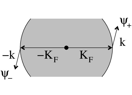
Refer to caption
Figure 1: The right-moving and left-moving modes near the Fermi surface can be combined into a two-component Dirac fermion.

We consider a theory where two patches of Fermi surface are coupled with one critical boson in (2+1)(2+1)-dimensions,

S\displaystyle S =\displaystyle= ∑s=±∑j=1N∫d3​k(2​π)3ψs,j†(k)[ik0+sk1+k22]ψs,j(k)\displaystyle\sum_{s=\pm}\sum_{j=1}^{N}\int\frac{d^{3}k}{(2\pi)^{3}}\psi_{s,j}^{\dagger}(k)\Bigl[ik_{0}+sk_{1}+k_{2}^{2}\Bigr]\psi_{s,j}(k) (1)
+\displaystyle+ 12​∫d3​k(2​π)3​[k02+k12+k22]​ϕ​(−k)​ϕ​(k)\displaystyle\frac{1}{2}\int\frac{d^{3}k}{(2\pi)^{3}}\left[k_{0}^{2}+k_{1}^{2}+k_{2}^{2}\right]\phi(-k)\phi(k)
+\displaystyle+ eN∑s=±∑j=1N∫d3​k​d3​q(2​π)6λsϕ(q)ψs,j†(k+q)ψs,j(k).\displaystyle\frac{e}{\sqrt{N}}\sum_{s=\pm}\sum_{j=1}^{N}\int\frac{d^{3}kd^{3}q}{(2\pi)^{6}}~\lambda_{s}~\phi(q)~\psi^{\dagger}_{s,j}(k+q)\psi_{s,j}(k).

Here ψ+,j\psi_{+,j} (ψ−,j\psi_{-,j}) is the right (left) moving fermion with flavor j=1,2,..,Nj=1,2,..,N whose Fermi velocity along the k1k_{1} direction is positive (negative). The momenta are rescaled in such a way that the absolute value of Fermi velocity and curvature of the Fermi surface are equal to one. ϕ\phi is a real critical boson, and ee is the fermion-boson coupling. Although the velocity of boson is in general different from that of fermion, the dynamics of boson is dominated by particle-hole excitations of fermion at low energies. As a result, the bare velocity of boson, which is also set to be one in the action, does not matter for the low energy effective theory. λs\lambda_{s} controls the way the fermions are coupled with the boson. The case with λ+=λ−=1\lambda_{+}=\lambda_{-}=1 describes the Ising-nematic critical point. The coupling with λ+=−λ−=1\lambda_{+}=-\lambda_{-}=1 describes the quantum electrodynamics at a finite density, where ϕ\phi corresponds to the transverse component of the U(1) gauge field. The action in Eq. (1) admits a self-contained renormalization group analysis[39].

In the following, we will focus on the Ising-nematic critical point. Quantum phase transitions to nematic states with broken point group symmetry[46] have been observed in cuprate superconductors[47, 48, 49, 50], ruthenades[51], and pnictides[52, 53, 54, 55]. The Ising-nematic order parameter is represented by a real scalar boson which undergoes strong quantum fluctuations at the quantum critical point.

Because the energy of fermion disperses only in one direction near the Fermi surface, the (2+1)(2+1)-dimensional fermion can be viewed as (1+1)(1+1)-dimensional Dirac fermions, where the momentum along the Fermi surface is interpreted as a continuous flavor. To make this more precise, the right and left moving fermions are combined into one spinor (see Fig. 1),

Ψj​(k)=(ψ+,j​(k)ψ−,j†​(−k)).\displaystyle\Psi_{j}(k)=\left(\begin{array}[]{c}\psi_{+,j}(k)\\ \psi_{-,j}^{\dagger}(-k)\end{array}\right).

In this representation, the action in Eq. (1) becomes

S\displaystyle S =\displaystyle= ∑j∫d3​k(2​π)3​Ψ¯j​(k)​[i​k0​γ0+i⁡(k1+k22)​γ1]​Ψj​(k)\displaystyle\sum_{j}\int\frac{d^{3}k}{(2\pi)^{3}}\bar{\Psi}_{j}(k)\Bigl[ik_{0}\gamma_{0}+i(k_{1}+k_{2}^{2})\gamma_{1}\Bigr]\Psi_{j}(k) (5)
+\displaystyle+ 12​∫d3​k(2​π)3​[k02+k12+k22]​ϕ​(−k)​ϕ​(k)\displaystyle\frac{1}{2}\int\frac{d^{3}k}{(2\pi)^{3}}\left[k_{0}^{2}+k_{1}^{2}+k_{2}^{2}\right]\phi(-k)\phi(k)
+\displaystyle+ eN​∑j∫d3​k​d​q(2​π)6​ϕ​(q)​Ψ¯j​(k+q)​W​Ψj​(k),\displaystyle\frac{e}{\sqrt{N}}\sum_{j}\int\frac{d^{3}kdq}{(2\pi)^{6}}\phi(q)\bar{\Psi}_{j}(k+q)W\Psi_{j}(k),

where γ0=σy\gamma_{0}=\sigma_{y}, γ1=σx\gamma_{1}=\sigma_{x} are the gamma matrices for the two component spinor, and Ψ¯≡Ψ†​γ0\bar{\Psi}\equiv\Psi^{\dagger}\gamma_{0}. W=i​γ1W=i\gamma_{1} (W=γ0W=\gamma_{0}) for the Ising-nematic system (quantum electrodynamics). For the rest of the paper, we will focus on the Ising-nematic case. The fermionic kinetic term is indeed identical to that of the (1+1)(1+1)-dimensional Dirac fermion where the location of Dirac point depends on k2k_{2}.

Refer to caption
Figure 2: (a) The one-dimensional Fermi surface embedded in the dd-dimensional momentum space. (b) For each kdk_{d}, there is a Fermi point at (k1,k2,…,kd−2,kd−1)=(0,0,..,0,−d−1kd2)(k_{1},k_{2},...,k_{d-2},k_{d-1})=(0,0,..,0,-\sqrt{d-1}k_{d}^{2}) which is denoted as a (red) dot. Around the Fermi point, the energy disperses linearly like a two-component Dirac fermion in (d−1)(d-1)-dimensional space.

Now we promote the theory to general dimensions. The action that describes Fermi surface with a general co-dimension is written as

S\displaystyle S =\displaystyle= ∑j∫dd+1​k(2​π)d+1​Ψ¯j​(k)​[i​𝚪⋅𝐊+i​γd−1​δk]​Ψj​(k)\displaystyle\sum_{j}\int\frac{d^{d+1}k}{(2\pi)^{d+1}}\bar{\Psi}_{j}(k)\Bigl[i{\mathbf{\Gamma}}\cdot{\mathbf{K}}+i\gamma_{d-1}\delta_{k}\Bigr]\Psi_{j}(k) (6)
+\displaystyle+ 12​∫dd+1​k(2​π)d+1​[|𝐊|2+kd−12+kd2]​ϕ​(−k)​ϕ​(k)\displaystyle\frac{1}{2}\int\frac{d^{d+1}k}{(2\pi)^{d+1}}\left[|{\mathbf{K}}|^{2}+k_{d-1}^{2}+k_{d}^{2}\right]\phi(-k)\phi(k)
+\displaystyle+ i​eN​d−1​∑j∫dd+1​k​dd+1​q(2​π)2​d+2​ϕ​(q)​Ψ¯j​(k+q)​γd−1​Ψj​(k).\displaystyle\frac{ie}{\sqrt{N}}\sqrt{d-1}\sum_{j}\int\frac{d^{d+1}kd^{d+1}q}{(2\pi)^{2d+2}}\phi(q)\bar{\Psi}_{j}(k+q)\gamma_{d-1}\Psi_{j}(k).

Here 𝐊≡(k0,k1,…,kd−2){\mathbf{K}}\equiv(k_{0},k_{1},\ldots,k_{d-2}) represents frequency and (d−2)(d-2) components of the full (d+1)(d+1)-dimensional energy-momentum vector, (k0,k1,…,kd)(k_{0},k_{1},...,k_{d}). k1,..,kd−2k_{1},..,k_{d-2} are the newly added directions which are transverse to the Fermi surface. δk=kd−1+d−1​kd2\delta_{k}=k_{d-1}+\sqrt{d-1}k_{d}^{2} is the energy dispersion of the fermion within the original two-dimensional momentum space. The gamma matrices associated with 𝐊{\mathbf{K}} are written as 𝚪≡(γ0,γ1,…,γd−2){\mathbf{\Gamma}}\equiv(\gamma_{0},\gamma_{1},\ldots,\gamma_{d-2}). Since the actual space dimension of interest lies between 22 and 33, the number of spinor components is fixed to be two. We will use the representation where γ0=σy\gamma_{0}=\sigma_{y} and γd−1=σx\gamma_{d-1}=\sigma_{x} are fixed in general dimensions.

The spinor has the energy dispersion with two bands,

Ek=±∑i=1(d−2)ki2+δk2.\displaystyle E_{k}=\pm\sqrt{\sum_{i=1}^{(d-2)}k_{i}^{2}+\delta_{k}^{2}}. (7)

The energy vanishes if

ki\displaystyle k_{i} =\displaystyle= 0,for​i=1,…,d−2\displaystyle 0,\qquad\mbox{for}\,\,\,i=1,\ldots,d-2\,
kd−1\displaystyle{k}_{d-1} =\displaystyle= −d−1​kd2.\displaystyle-\sqrt{d-1}k_{d}^{2}. (8)

Therefore the Fermi surface is a one-dimensional manifold embedded in the dd-dimensional momentum space as is shown in Fig. 2.

Refer to caption
Figure 3: Fermi lines in three dimensional momentum space can be obtained by turning on pp-wave superconducting order parameter that gaps out the cylindrical Fermi surface except for the line node denoted by the thick (red) line.

Before we delve into the RG analysis in an abstract dimension dd, we consider a concrete physical realization of the theory in d=3d=3 with N=2N=2, where two flavors represent spin 1/21/2 degree of freedom. In the basis where γ0=σy\gamma_{0}=\sigma_{y}, γ1=σz\gamma_{1}=\sigma_{z}, γ2=σx\gamma_{2}=\sigma_{x}, the quadratic action for the fermions becomes

S\displaystyle S =\displaystyle= ∫d4​k(2​π)3{∑s=±∑j=↑,↓ψs,j†(k)(ik0+sk2+2k32)ψs,j(k)\displaystyle\int\frac{d^{4}k}{(2\pi)^{3}}\Bigg\{\sum_{s=\pm}\sum_{j=\uparrow,\downarrow}\psi_{s,j}^{\dagger}(k)\left(ik_{0}+sk_{2}+\sqrt{2}k_{3}^{2}\right)\psi_{s,j}(k) (9)
−k1(ψ+,↑†(k)ψ−,↑†(−k)+ψ+,↓†(k)ψ−,↓†(−k)+h.c.)}.\displaystyle-k_{1}\left(\psi_{+,\uparrow}^{\dagger}(k)\psi_{-,\uparrow}^{\dagger}(-k)+\psi_{+,\downarrow}^{\dagger}(k)\psi_{-,\downarrow}^{\dagger}(-k)+h.c.\right)\Bigg\}.

The last term represents a pairing which can be written as

i⁡(ψ+,↑†​(k),ψ+,↓†​(k))​(𝐝⁡(k)⋅𝝈)​σy​(ψ−,↑†​(−k)ψ−,↓†​(−k))+h.c.\displaystyle i\Bigl(\psi_{+,\uparrow}^{\dagger}(k),\psi_{+,\downarrow}^{\dagger}(k)\Bigr)\Bigl({\mathbf{d}}(k)\cdot\boldsymbol{\sigma}\Bigr)\sigma_{y}\left(\begin{array}[]{c}\psi_{-,\uparrow}^{\dagger}(-k)\\ \psi_{-,\downarrow}^{\dagger}(-k)\end{array}\right)+h.c.

with 𝐝⁡(k)=i​k1​y^{\mathbf{d}}(k)=ik_{1}\hat{y}. It is noted that 𝐝⁡(k){\mathbf{d}}(k) transforms as a vector under S​U​(2)SU(2) spin rotations. Therefore this describes a pp-wave spin triplet superconducting state. Without the pairing term, one has the cylindrical Fermi surface with co-dimension one at ±k2+2​k32=0\pm k_{2}+\sqrt{2}k_{3}^{2}=0. The pairing gaps out the Fermi surface except for the line node at k1=0k_{1}=0. This is illustrated in Fig. 3. The triplet pairing breaks the U⁡(1)U(1) symmetry associated with the fermion number conservation to Z2Z_{2} and the S​U​(2)SU(2) spin rotational symmetry to U⁡(1)U(1). The theories in general dimensions continuously interpolate the Fermi surface in two dimensions to the triplet superconducting state in three dimensions. In terms of symmetry, the theory in d=2d=2 is a special point with an enhanced symmetry.

III Renormalization Group

III.1 Minimal Action

To start with a renormalization group analysis, we first focus on the quadratic action in Eq. (6). The leading terms in the quadratic action are invariant under the scale transformation,

𝐊\displaystyle{\mathbf{K}} =\displaystyle= 𝐊′b,\displaystyle\frac{{\mathbf{K}}^{\prime}}{b}, (13)
kd−1\displaystyle k_{d-1} =\displaystyle= kd−1′b,\displaystyle\frac{k_{d-1}^{\prime}}{b}, (14)
kd\displaystyle k_{d} =\displaystyle= kd′b,\displaystyle\frac{k_{d}^{\prime}}{\sqrt{b}}, (15)
Ψ⁡(k)\displaystyle\Psi(k) =\displaystyle= bd2+34​Ψ′​(k′),\displaystyle b^{\frac{d}{2}+\frac{3}{4}}\Psi^{\prime}(k^{\prime}), (16)
ϕ⁡(k)\displaystyle\phi(k) =\displaystyle= bd2+34​ϕ′​(k′).\displaystyle b^{\frac{d}{2}+\frac{3}{4}}\phi^{\prime}(k^{\prime}). (17)

Under the scaling with b>1b>1, the fermion-boson coupling scales as

e′=b12​(52−d)​e.e^{\prime}=b^{\frac{1}{2}(\frac{5}{2}-d)}e. (18)

The coupling ee is irrelevant for d>dcr=5/2d>d_{{\rm cr}}=5/2, and is relevant for d<5/2d<5/2. This allows one to access an interacting non-Fermi liquid state perturbatively in d=5/2−ϵd=5/2-\epsilon using ϵ\epsilon as a small parameter.

We note that |𝐊|2​ϕ∗​(k)​ϕ​(k)|{\mathbf{K}}|^{2}\phi^{*}(k)\phi(k) and kd−12​ϕ∗​(k)​ϕ​(k)k_{d-1}^{2}\phi^{*}(k)\phi(k) are irrelevant in the low energy limit. Only kd2​ϕ∗​(k)​ϕ​(k)k_{d}^{2}\phi^{*}(k)\phi(k) is kept in the quadratic action of the boson. The frequency dependent self energy of the boson will be dynamically generated by particle-hole fluctuations. Therefore, the minimal local action is given by

S\displaystyle S =\displaystyle= ∑j∫dd+1​k(2​π)d+1​Ψ¯j​(k)​[i​𝚪⋅𝐊+i​γd−1​δk]​Ψj​(k)\displaystyle\sum_{j}\int\frac{d^{d+1}k}{(2\pi)^{d+1}}\bar{\Psi}_{j}(k)\Bigl[i{\mathbf{\Gamma}}\cdot{\mathbf{K}}+i\gamma_{d-1}\delta_{k}\Bigr]\Psi_{j}(k) (19)
+\displaystyle+ 12​∫dd+1​k(2​π)d+1​kd2​ϕ​(−k)​ϕ​(k)\displaystyle\frac{1}{2}\int\frac{d^{d+1}k}{(2\pi)^{d+1}}~~k_{d}^{2}\phi(-k)\phi(k)
+\displaystyle+ i​e​μϵ/2N​d−1​∑j∫dd+1​k​dd+1​q(2​π)2​d+2​ϕ​(q)​Ψ¯j​(k+q)​γd−1​Ψj​(k),\displaystyle\frac{ie\mu^{\epsilon/2}}{\sqrt{N}}\sqrt{d-1}\sum_{j}\int\frac{d^{d+1}kd^{d+1}q}{(2\pi)^{2d+2}}\phi(q)\bar{\Psi}_{j}(k+q)\gamma_{d-1}\Psi_{j}(k),

where a mass scale μ\mu is introduced to make the coupling constant dimensionless. Short-ranged four fermion interactions and the ϕ4\phi^{4} term for the boson are not included in the minimal action because they are irrelevant near d=5/2d=5/2. There is no further BCS instability that gaps out the line nodes near d=5/2d=5/2 because the density of state vanishes at Fermi energy.

For d>5/2d>5/2, the interaction is irrelevant and the low energy physics is governed by the scaling in Eqs. (13)-(17) with the dynamical critical exponent z=1z=1. For d<5/2d<5/2, the scaling will be modified such that the interaction plays the dominant role. In order to see this, one can choose an alternative scaling,

𝐊\displaystyle{\mathbf{K}} =\displaystyle= 𝐊′bz,\displaystyle\frac{{\mathbf{K}}^{\prime}}{b^{z}}, (20)
kd−1\displaystyle k_{d-1} =\displaystyle= kd−1′b,\displaystyle\frac{k_{d-1}^{\prime}}{b}, (21)
kd\displaystyle k_{d} =\displaystyle= kd′b,\displaystyle\frac{k_{d}^{\prime}}{\sqrt{b}}, (22)
Ψ⁡(k)\displaystyle\Psi(k) =\displaystyle= b(d−1)​z2+54​Ψ′​(k′),\displaystyle b^{\frac{(d-1)z}{2}+\frac{5}{4}}\Psi^{\prime}(k^{\prime}), (23)
ϕ⁡(k)\displaystyle\phi(k) =\displaystyle= b(d−1)​z2+54​ϕ′​(k′).\displaystyle b^{\frac{(d-1)z}{2}+\frac{5}{4}}\phi^{\prime}(k^{\prime}). (24)

The condition that the interaction is kept marginal at the expense of making the first quadratic term in Eq. (19) irrelevant uniquely fixes the dynamical critical exponent to be z=33−2​ϵz=\frac{3}{3-2\epsilon} at the tree level. As will be shown later, this is indeed what we obtain from a full-fledged computation modulo a correction coming from the anomalous dimension of the boson field.

III.2 Symmetry

In this section, we discuss about the symmetry of the action in Eq. (19). The (2+1)(2+1)-dimensional theory in Eq. (5) has two classical U⁡(N)U(N) symmetries given by

UA​(N):Ψi\displaystyle U_{A}(N):\Psi_{i} →\displaystyle\rightarrow [ei​θα​Tα]i​j​Ψj,\displaystyle[e^{i\theta_{\alpha}T^{\alpha}}]_{ij}\Psi_{j}, (25)
UB​(N):Ψi\displaystyle U_{B}(N):\Psi_{i} →\displaystyle\rightarrow [ei​σz​φα​Tα]i​j​Ψj,\displaystyle[e^{i\sigma_{z}\varphi_{\alpha}T^{\alpha}}]_{ij}\Psi_{j}, (26)

where TαT^{\alpha} with α=1,2,..,N2\alpha=1,2,..,N^{2} represent N×NN\times N Hermitian matrices. UA​(N)U_{A}(N) and UB​(N)U_{B}(N) respectively correspond to the global and axial symmetry groups of the underlying (1+1)(1+1)-dimensional theory when k2k_{2} is interpreted as an internal flavor. The generators of the two U⁡(N)U(N) groups are given by

jA​0α\displaystyle j_{A0}^{\alpha} =\displaystyle= ψ+,i†​Ti​jα​ψ+,j−ψ−,i†​(Tα)i​jT​ψ−,j,\displaystyle\psi_{+,i}^{\dagger}T_{ij}^{\alpha}\psi_{+,j}-\psi_{-,i}^{\dagger}(T^{\alpha})^{T}_{ij}\psi_{-,j}, (27)
jB​0α\displaystyle j_{B0}^{\alpha} =\displaystyle= ψ+,i†​Ti​jα​ψ+,j+ψ−,i†​(Tα)i​jT​ψ−,j,\displaystyle\psi_{+,i}^{\dagger}T^{\alpha}_{ij}\psi_{+,j}+\psi_{-,i}^{\dagger}(T^{\alpha})^{T}_{ij}\psi_{-,j}, (28)

where (Tα)T(T^{\alpha})^{T} denotes the transpose of TαT^{\alpha}. In general dimensions, only the UA​(N)U_{A}(N) symmetry is kept. The axial UB​(N)U_{B}(N) symmetry is absent in d>2d>2 because fermions with opposite chiralities are mixed. The inability to keep both symmetries is related to the chiral anomaly in (1+1)(1+1) dimensions.

The theory in general dimensions retain the Ward identity and the sliding symmetry of the (2+1)(2+1)-dimensional theory[39]. In the Ising-nematic case, the boson couples to the (d−1)(d-1)-th component of the UA​(1)U_{A}(1) current. This implies the Ward identity

Γ⁡(k,0)\displaystyle\Gamma(k,0) =\displaystyle= ∂G−1​(k)∂kd−1,\displaystyle\frac{\partial G^{-1}(k)}{\partial k_{d-1}}, (29)

where Γ⁡(k,q)\Gamma(k,q) is the fermion-boson vertex function, and G⁡(k)G(k) is the fermion propagator. The theory also has the sliding symmetry along the Fermi surface given by

Ψ⁡(𝐊,kd−1,kd)\displaystyle\Psi({\mathbf{K}},k_{d-1},k_{d}) →\displaystyle\rightarrow Ψ⁡(𝐊,kd−1−d−1​(2​θ​kd+θ2),kd+θ),\displaystyle\Psi({\mathbf{K}},k_{d-1}-\sqrt{d-1}(2\theta k_{d}+\theta^{2}),k_{d}+\theta),
ϕ⁡(𝐐,qd−1,qd)\displaystyle\phi({\mathbf{Q}},q_{d-1},q_{d}) →\displaystyle\rightarrow ϕ⁡(𝐐,qd−1−2​d−1​θ​qd,qd).\displaystyle\phi({\mathbf{Q}},q_{d-1}-2\sqrt{d-1}\theta q_{d},q_{d}). (30)

As a result, the fermion propagator depends on kd−1k_{d-1} and kdk_{d} only through δk\delta_{k}, and the boson propagator is independent of qd−1q_{d-1},

G⁡(𝐊,kd−1,kd)\displaystyle G({\mathbf{K}},k_{d-1},k_{d}) =\displaystyle= G⁡(𝐊,δk),\displaystyle G({\mathbf{K}},\delta_{k}),
D⁡(𝐐,qd−1,qd)\displaystyle D({\mathbf{Q}},q_{d-1},q_{d}) =\displaystyle= D⁡(𝐐,qd).\displaystyle D({\mathbf{Q}},q_{d}). (31)

Finally, the action respects the (d−1)(d-1)-dimensional rotational symmetry in the space of 𝐊{\mathbf{K}} and the time-reversal symmetry.

III.3 Renormalization Group Equation

Refer to caption
Figure 4: The one-loop boson self-energy.

We use the field theoretical renormalization group approach to study the scaling behaviour of the theory in d<5/2d<5/2, using ϵ=52−d\epsilon=\frac{5}{2}-d as a perturbative parameter. At each order in the loop expansion, we add counter terms to cancel divergent terms in 1/ϵ1/\epsilon using the minimal subtraction scheme. The bare propagator for fermions is given by

G0​(k)=1i​𝚪⋅𝐊+γd−1​δk𝐊2+δk2.G_{0}(k)=\frac{1}{i}\,\frac{{\mathbf{\Gamma}}\cdot{\mathbf{K}}+\gamma_{d-1}\delta_{k}}{{\mathbf{K}}^{2}+\delta_{k}^{2}}. (32)

Since the bare kinetic term of boson depends only on kdk_{d}, one has to include the lowest order quantum correction to ensure IR and UV finiteness. Therefore, we use the dressed propagator for boson which includes the one-loop self-energy as is shown in Fig. 4,

D1​(k)=1kd2−Π1​(k)=1kd2+βd​e2​μϵ​|𝐊|d−1|kd|,D_{1}(k)=\frac{1}{k_{d}^{2}-\Pi_{1}(k)}=\frac{1}{k_{d}^{2}+\beta_{d}e^{2}\mu^{\epsilon}\frac{|{\mathbf{K}}|^{d-1}}{|k_{d}|}}, (33)

where

βd=d−1​Γ2​(d/2)2d​π(d−1)/2​|cos⁡(π​d/2)|​Γ​(d−12)​Γ​(d).\beta_{d}=\frac{\sqrt{d-1}\Gamma^{2}(d/2)}{2^{d}\pi^{(d-1)/2}\,|\cos(\pi d/2)|\,\Gamma(\frac{d-1}{2})\Gamma(d)}. (34)

We use the sign convention where the self energy subtract the bare action in the dressed propagator as D⁡(k)=1D1−1​(k)−Π⁡(k)D(k)=\frac{1}{D_{1}^{-1}(k)-\Pi(k)}, G⁡(k)=1G0−1​(k)−Σ⁡(k)G(k)=\frac{1}{G_{0}^{-1}(k)-\Sigma(k)}, where Π⁡(k)\Pi(k) and Σ⁡(k)\Sigma(k) are the self energies of boson and fermion respectively. The one-loop boson self-energy Π1​(k)\Pi_{1}(k) is finite for 2≤d<32\leq d<3. At d=5/2d=5/2, it has the same scaling dimension as kd2k_{d}^{2} as expected. For computation of Π1​(k)\Pi_{1}(k), see Appendix A.1.

We note that the inclusion of the one-loop boson self energy in the zero-th order quantum effective action is nothing but a rearrangement in the perturbative expansion of a local theory. This is because the non-local self energy is dynamically generated from the local action. The fact that the one-loop boson self energy has to be included from the beginning has some consequences. First, the ‘loop-expansion’ we are going to use is defined modulo the inclusion of the one-loop self energy of boson. For examples, the diagrams in Fig. 5 are regarded as one-loop diagrams although the boson propagators in the diagrams already include the RPA sum of boson self energy. Second, the dynamics of boson has a intrinsic crossover scale at kd∼e2/3​|𝐊|(d−1)/3k_{d}\sim e^{2/3}|{\mathbf{K}}|^{(d-1)/3} which goes to zero in the weak coupling limit. Because of this, the actual parameter that controls the loop expansion is not ee as will be discussed in Sec. III D in more detail.

The counter terms take the same form as the original local action,

SC​T\displaystyle S_{CT} =\displaystyle= ∑j∫dd+1​k(2​π)d+1​Ψ¯j​(k)​[i​A1​𝚪⋅𝐊+i​A2​γd−1​δk]​Ψj​(k)\displaystyle\sum_{j}\int\frac{d^{d+1}k}{(2\pi)^{d+1}}\bar{\Psi}_{j}(k)\Bigl[iA_{1}{\mathbf{\Gamma}}\cdot{\mathbf{K}}+iA_{2}\gamma_{d-1}\delta_{k}\Bigr]\Psi_{j}(k) (35)
+\displaystyle+ A32​∫dd+1​k(2​π)d+1​kd2​ϕ​(−k)​ϕ​(k)\displaystyle\frac{A_{3}}{2}\int\frac{d^{d+1}k}{(2\pi)^{d+1}}~~k_{d}^{2}\phi(-k)\phi(k)
+\displaystyle+ A4​i​e​μϵ/2N​d−1​∑j∫dd+1​k​dd+1​q(2​π)2​d+2​ϕ​(q)​Ψ¯j​(k+q)​γd−1​Ψj​(k),\displaystyle A_{4}\frac{ie\mu^{\epsilon/2}}{\sqrt{N}}\sqrt{d-1}\sum_{j}\int\frac{d^{d+1}kd^{d+1}q}{(2\pi)^{2d+2}}\phi(q)\bar{\Psi}_{j}(k+q)\gamma_{d-1}\Psi_{j}(k),

where

An=∑k=1∞Zn,k​(e)ϵk.A_{n}=\sum_{k=1}^{\infty}\frac{Z_{n,k}(e)}{\epsilon^{k}}. (36)

In the mass independent minimal subtraction scheme, the coefficients Zn,k​(e)Z_{n,k}(e) depend only on the coupling. AnA_{n} and Zn,kZ_{n,k} can be further expanded in the number of loops. We use An(L)A_{n}^{(L)} and Zn,k(L)Z_{n,k}^{(L)} to denote LL-loop contributions modulo the one-loop self energy of boson which is already included in Eq. (33). Note that the (d−1)(d-1)-dimensional rotational invariance in the space perpendicular to the Fermi surface guarantees that Γi​Ki\Gamma_{i}K_{i} are renormalized in the same way for 0≤i≤(d−2)0\leq i\leq(d-2). Similarly, the sliding symmetry along the Fermi surface guarantees that the form of δk\delta_{k} is preserved. However, A1A_{1} and A2A_{2} are in general different due to a lack of the full rotational symmetry in the (d+1)(d+1)-dimensional spacetime. This will leads to a non-trivial dynamical critical exponent as will be shown later. The Ward identity in Eq. (29) forces A4=A2A_{4}=A_{2}.

Adding the counter terms to the original action, we obtain the renormalized action which gives the finite quantum effective action,

Sr​e​n\displaystyle S_{ren} =\displaystyle= ∑j∫dd+1​kB(2​π)d+1​Ψ¯B​j​(kB)​[i​𝚪⋅𝐊B+i​γd−1​δkB]​ΨB​j​(kB)\displaystyle\sum_{j}\int\frac{d^{d+1}k_{B}}{(2\pi)^{d+1}}\bar{\Psi}_{Bj}(k_{B})\Bigl[i{\mathbf{\Gamma}}\cdot{\mathbf{K}}_{B}+i\gamma_{d-1}\delta_{k_{B}}\Bigr]\Psi_{Bj}(k_{B}) (37)
+\displaystyle+ 12​∫dd+1​kB(2​π)d+1​kB​d2​ϕB​(−kB)​ϕB​(kB)\displaystyle\frac{1}{2}\int\frac{d^{d+1}k_{B}}{(2\pi)^{d+1}}~k_{Bd}^{2}\phi_{B}(-k_{B})\phi_{B}(k_{B})
+\displaystyle+ i​eBN​d−1​∑j∫dd+1​kB​dd+1​qB(2​π)2​d+2​ϕB​(qB)​Ψ¯B​j​(kB+qB)​γd−1​ΨB​j​(kB),\displaystyle\frac{ie_{B}}{\sqrt{N}}\sqrt{d-1}\sum_{j}\int\frac{d^{d+1}k_{B}d^{d+1}q_{B}}{(2\pi)^{2d+2}}\phi_{B}(q_{B})\bar{\Psi}_{Bj}(k_{B}+q_{B})\gamma_{d-1}\Psi_{Bj}(k_{B}),

where

𝐊\displaystyle{\mathbf{K}} =\displaystyle= Z2Z1​𝐊B,\displaystyle\frac{Z_{2}}{Z_{1}}{\mathbf{K}}_{B},
kd−1\displaystyle k_{d-1} =\displaystyle= kB,d−1,\displaystyle k_{B,d-1},
kd\displaystyle k_{d} =\displaystyle= kB,d,\displaystyle k_{B,d},
Ψ⁡(k)\displaystyle\Psi(k) =\displaystyle= ZΨ−1/2ΨB(kB),\displaystyle Z_{\Psi}^{-1/2}\Psi_{B}(k_{B}),
ϕ⁡(k)\displaystyle\phi(k) =\displaystyle= Zϕ−1/2ϕB(kB),\displaystyle Z_{\phi}^{-1/2}\phi_{B}(k_{B}),
eB\displaystyle e_{B} =\displaystyle= Z3−1/2(Z2Z1)(d−1)/2μϵ/2e\displaystyle Z_{3}^{-1/2}\left(\frac{Z_{2}}{Z_{1}}\right)^{(d-1)/2}\mu^{\epsilon/2}e (38)

with Zn=1+AnZ_{n}=1+A_{n}, ZΨ=Z2​(Z2Z1)(d−1)Z_{\Psi}=Z_{2}\left(\frac{Z_{2}}{Z_{1}}\right)^{(d-1)} and Zϕ=Z3​(Z2Z1)(d−1)Z_{\phi}=Z_{3}\left(\frac{Z_{2}}{Z_{1}}\right)^{(d-1)}. In Eq. (37), there is a freedom to change the renormalizations of the fields and the renormalization of momentum without affecting the action. Here we fix the freedom by requiring that δkB=δk\delta_{k_{B}}=\delta_{k}. This amounts to measuring scaling dimensions of all other quantities relative to that of δk\delta_{k}.

The finite renormalized Green’s function is defined by

⟨Ψ¯​(k1)..Ψ¯​(km)​Ψ​(km+1)..Ψ⁡(k2​m)​ϕ​(k2​m+1)..ϕ⁡(k2​m+n)⟩\displaystyle\Bigl<\bar{\Psi}(k_{1})..\bar{\Psi}(k_{m})~\Psi(k_{m+1})..\Psi(k_{2m})~\phi(k_{2m+1})..\phi(k_{2m+n})\Bigr>
=G(m,m,n)​({ki},e,μ)​δd+1​(∑i=1mki−∑j=m+12​m+nkj),\displaystyle=G^{(m,m,n)}(\{k_{i}\};e,\mu)~~\delta^{d+1}\left(\sum_{i=1}^{m}k_{i}-\sum_{j=m+1}^{2m+n}k_{j}\right), (39)

where the flavor and spacetime indices of fermions are suppressed. It is related to the bare Green’s function defined by

⟨Ψ¯B​(kB​1)..Ψ¯B​(kB​m)​ΨB​(kB​m+1)..ΨB​(kB​2​m)​ϕB​(kB​2​m+1)..ϕB​(kB​2​m+n)⟩\displaystyle\Bigl<\bar{\Psi}_{B}(k_{B1})..\bar{\Psi}_{B}(k_{Bm})~\Psi_{B}(k_{Bm+1})..\Psi_{B}(k_{B2m})~\phi_{B}(k_{B2m+1})..\phi_{B}(k_{B2m+n})\Bigr>
=GB(m,m,n)​({kB​i},eB)​δd+1​(∑i=1mkB​i−∑j=m+12​m+nkB​j),\displaystyle=G_{B}^{(m,m,n)}(\{k_{Bi}\};e_{B})~~\delta^{d+1}\left(\sum_{i=1}^{m}k_{Bi}-\sum_{j=m+1}^{2m+n}k_{Bj}\right), (40)

through the multiplicative renormalization,

G(m,m,n)​({ki},e,μ)=ZΨ−m​Zϕ−n2​(Z2Z1)d−1​GB(m,m,n)​({kB​i},eB).\displaystyle G^{(m,m,n)}(\{k_{i}\};e,\mu)=Z_{\Psi}^{-m}Z_{\phi}^{-\frac{n}{2}}\left(\frac{Z_{2}}{Z_{1}}\right)^{d-1}G_{B}^{(m,m,n)}(\{k_{Bi}\};e_{B}). (41)

Using the facts that the bare Green’s function is independent of μ\mu and that G(m,m,n)G^{(m,m,n)} has the engineering scaling dimension −(2​m+n)​4−ϵ2+(3−ϵ)-(2m+n)\frac{4-\epsilon}{2}+(3-\epsilon), one obtains the renormalization group equation,

{∑i=12​m+n(z(e)𝐊i⋅∇Ki+ki,d−1∂∂ki,d−1+ki,d2∂∂ki,d)−β(e)∂∂e−2m[−4−ϵ2+ηψ]\displaystyle\Bigg\{\sum_{i=1}^{2m+n}\left(z(e)\,{\mathbf{K}}_{i}\cdot\nabla_{K_{i}}+k_{i,d-1}\frac{\partial}{\partial k_{i,d-1}}+\frac{k_{i,d}}{2}\frac{\partial}{\partial k_{i,d}}\right)-\beta(e)\frac{\partial}{\partial e}-2m\left[-\frac{4-\epsilon}{2}+\eta_{\psi}\right]
−n[−4−ϵ2+ηϕ]−[z(e)(32−ϵ)+32]}G(m,m,n)({ki};e,μ)=0.\displaystyle-n\left[-\frac{4-\epsilon}{2}+\eta_{\phi}\right]-\left[z(e)\left(\frac{3}{2}-\epsilon\right)+\frac{3}{2}\right]\Bigg\}G^{(m,m,n)}(\{k_{i}\};e,\mu)=0. (42)

From the equation, it is clear that the dimension of 𝐊{\mathbf{K}} is renormalized to zz, and the total dimension of spacetime becomes −[z⁡(32−ϵ)+32]-\left[z\left(\frac{3}{2}-\epsilon\right)+\frac{3}{2}\right] accordingly. Here zz is the dynamical critical exponent, β\beta is the beta function, and ηψ\eta_{\psi} (ηϕ\eta_{\phi}) is the anomalous dimensions for fermion (boson) which are given by

z⁡(e)\displaystyle z(e) =\displaystyle= 1−∂ln⁡(Z2/Z1)∂ln⁡μ,\displaystyle 1-\frac{\partial\ln(Z_{2}/Z_{1})}{\partial\ln\mu},
β⁡(e)\displaystyle\beta(e) =\displaystyle= ∂e∂ln⁡μ,\displaystyle\frac{\partial e}{\partial\ln\mu},
ηψ​(e)\displaystyle\eta_{\psi}(e) =\displaystyle= 12​∂ln⁡ZΨ∂ln⁡μ,\displaystyle\frac{1}{2}\frac{\partial\ln Z_{\Psi}}{\partial\ln\mu},
ηϕ​(e)\displaystyle\eta_{\phi}(e) =\displaystyle= 12​∂ln⁡Zϕ∂ln⁡μ.\displaystyle\frac{1}{2}\frac{\partial\ln Z_{\phi}}{\partial\ln\mu}. (43)

We use the convention that the beta function describes the flow of the coupling with increasing energy scale. These four equations can be rewritten as

β(Z1Z2′−Z2Z1′)+Z1Z2(z−1)\displaystyle\beta(Z_{1}Z_{2}^{{}^{\prime}}-Z_{2}Z_{1}^{{}^{\prime}})+Z_{1}Z_{2}(z-1) =\displaystyle= 0,\displaystyle 0,
e[−ϵ2z+34(z−1)]Z3−[Z3−e2Z3′]β\displaystyle e\left[-\frac{\epsilon}{2}z+\frac{3}{4}(z-1)\right]Z_{3}-\left[Z_{3}-\frac{e}{2}Z_{3}^{{}^{\prime}}\right]\beta =\displaystyle= 0,\displaystyle 0,
Z2ηψ−β2Z2′+(34−ϵ2)(z−1)Z2\displaystyle Z_{2}\eta_{\psi}-\frac{\beta}{2}Z_{2}^{{}^{\prime}}+\left(\frac{3}{4}-\frac{\epsilon}{2}\right)(z-1)Z_{2} =\displaystyle= 0,\displaystyle 0,
Z3ηϕ−β2Z3′+(34−ϵ2)(z−1)Z3\displaystyle Z_{3}\eta_{\phi}-\frac{\beta}{2}Z_{3}^{{}^{\prime}}+\left(\frac{3}{4}-\frac{\epsilon}{2}\right)(z-1)Z_{3} =\displaystyle= 0,\displaystyle 0, (44)

where primes represent derivatives with respect to ee. One can readily see that the regular part of Eqs. (43) in the ϵ→0\epsilon\rightarrow 0 limit requires the solutions of the form,

z\displaystyle z =\displaystyle= z(0),\displaystyle z^{(0)},
β\displaystyle\beta =\displaystyle= β(1)​ϵ+β(0),\displaystyle\beta^{(1)}\epsilon+\beta^{(0)},
ηψ\displaystyle\eta_{\psi} =\displaystyle= ηΨ(1)​ϵ+ηΨ(0),\displaystyle\eta_{\Psi}^{(1)}\epsilon+\eta_{\Psi}^{(0)},
ηϕ\displaystyle\eta_{\phi} =\displaystyle= ηϕ(1)​ϵ+ηϕ(0).\displaystyle\eta_{\phi}^{(1)}\epsilon+\eta_{\phi}^{(0)}. (45)

Using this form, one can solve Eqs. (44) at each order in ϵ\epsilon. z,β,ηψ,ηϕz,\beta,\eta_{\psi},\eta_{\phi} are determined from the simple poles of the counter terms as

z\displaystyle z =\displaystyle= 22+e(Z1,1′−Z2,1′),\displaystyle\frac{2}{2+e(Z_{1,1}^{{}^{\prime}}-Z_{2,1}^{{}^{\prime}})}, (46)
β\displaystyle\beta =\displaystyle= (−ϵ2z+34(z−1))e−z​e24Z3,1′,\displaystyle\left(-\frac{\epsilon}{2}z+\frac{3}{4}(z-1)\right)e-\frac{ze^{2}}{4}Z_{3,1}^{{}^{\prime}}, (47)
ηψ\displaystyle\eta_{\psi} =\displaystyle= −(z−1)​(3−2​ϵ)4−z​e4Z2,1′,\displaystyle-\frac{(z-1)(3-2\epsilon)}{4}-\frac{ze}{4}Z_{2,1}^{{}^{\prime}}, (48)
ηϕ\displaystyle\eta_{\phi} =\displaystyle= −(z−1)​(3−2​ϵ)4−z​e4Z3,1′.\displaystyle-\frac{(z-1)(3-2\epsilon)}{4}-\frac{ze}{4}Z_{3,1}^{{}^{\prime}}. (49)

In Eq. (46), we see that the dynamical critical exponent is renormalized by quantum effects. In other words, the first (d−1)(d-1) components of the energy-momentum vector acquires an anomalous dimension (z−1)(z-1). The anomalous dimension of spacetime affects the scaling dimension of the coupling and the anomalous dimensions of the fields in Eqs. (47), (48) and (49). Once Zn,m′Z_{n,m}^{{}^{\prime}} are computed, one can obtain the beta functions and the critical exponents.

The theory has the Gaussian fixed point at which e=0,z=1,ηψ=ηϕ=0e=0,z=1,\eta_{\psi}=\eta_{\phi}=0. As a small coupling is turned on, the theory flows to an interacting fixed point with e∗≠0e^{*}\neq 0 at low energies. The condition that the beta function vanishes at the interacting fixed point determines the dynamical critical exponent to be

z∗=33−2ϵ−e∗Z3,1′.\displaystyle z^{*}=\frac{3}{3-2\epsilon-e^{*}Z_{3,1}^{{}^{\prime}}}. (50)

It is remarkable that the dynamical critical exponent at the fixed point is independent of Z1Z_{1} and Z2Z_{2}. If Z3,1=0Z_{3,1}=0, z∗z^{*} is exactly given by z∗=33−2​ϵz^{*}=\frac{3}{3-2\epsilon} which monotonically increases from 11 to 3/23/2 as dd changes from 5/25/2 to 22. At the fixed point, the scaling dictates the form of the two-point functions as

D⁡(k)\displaystyle D(k) =\displaystyle= 1(kd2)1−(z−1)​(3/2−ϵ)−2​ηϕ​f​(|𝐊|1/zkd2),\displaystyle\frac{1}{(k_{d}^{2})^{1-(z-1)(3/2-\epsilon)-2\eta_{\phi}}}~~f\left(\frac{|{\mathbf{K}}|^{1/z}}{k_{d}^{2}}\right), (51)
G⁡(k)\displaystyle G(k) =\displaystyle= 1|δk|1−(z−1)​(3/2−ϵ)−2​ηψ​g​(|𝐊|1/zδk),\displaystyle\frac{1}{|\delta_{k}|^{1-(z-1)(3/2-\epsilon)-2\eta_{\psi}}}~~g\left(\frac{|{\mathbf{K}}|^{1/z}}{\delta_{k}}\right), (52)

where f⁡(x)f(x) and g⁡(x)g(x) are universal cross-over functions. The flavor and the spinor indices are suppressed in g⁡(x)g(x). If the anomalous dimensions are large enough, the singularity in the Green’s functions can in principle turn into an algebraic gap[56]. However, the anomalous dimensions are small near the upper critical dimension.

III.4 Expansion parameter

We take the small ϵ\epsilon limit with fixed NN. In this section, we show that the loop expansion is controlled in this limit. Although the bare fermion-boson vertex includes ee, it is not the actual expansion parameter. This is due to the fact that the boson propagator includes the self energy which vanishes in the e→0e\rightarrow 0 limit. To examine this issue more closely, let us consider a boson propagator which carries an internal momentum kk within a diagram. The integration over kk is of the form,

∫d​k​F​(k,{qi})​1kd2+βd​e2​μϵ​|𝐊|d−1|kd|,\displaystyle\int dk~F(k,\{q_{i}\})\frac{1}{k_{d}^{2}+\beta_{d}e^{2}\mu^{\epsilon}\frac{|{\mathbf{K}}|^{d-1}}{|k_{d}|}}, (53)

where {qi}\{q_{i}\} is a set of other internal and external momenta, and F⁡(k,{qi})F(k,\{q_{i}\}) represents the contribution from other propagators. When kdk_{d} can be arbitrarily small in magnitude, the integration is in general IR divergent in the e→0e\rightarrow 0 limit. The IR divergence is cut-off at a scale kd∼e2/3​|𝐊|(d−1)/3k_{d}\sim e^{2/3}|{\mathbf{K}}|^{(d-1)/3}, and the result of the integration becomes order of e−2/3e^{-2/3}. Therefore, each boson propagator contributes an IR enhancement factor of e−2/3e^{-2/3} provided that the internal momentum that runs through each boson propagator is allowed to vanish independently.

If there is a kinematic constraint that keeps kdk_{d} from becoming arbitrarily small in magnitude, kdk_{d} integration is convergent in the e→0e\rightarrow 0 limit. Then there is no IR enhancement factor. However, one still has to worry about UV divergence in the e→0e\rightarrow 0 limit. In particular, the integration over 𝐊{\mathbf{K}} can be UV divergent without the self energy in the boson propagator. In the presence of the self-energy, quantum corrections to marginal operators can have at most log divergences by power counting. In the e→0e\rightarrow 0 limit, they can have power-law UV divergences because the boson propagator no longer depends on 𝐊{\mathbf{K}}. The degree of UV divergence for marginal operators is at most IbI_{b}, where IbI_{b} is the number of internal boson propagators. This is because only the boson propagator depends on ee, and each boson propagator carries the scaling dimension −1-1. In the presence of the boson self energy, the power-law divergence is cut-off at a scale |𝐊|∼e−2/(d−1)kd3/(d−1)|{\mathbf{K}}|\sim e^{-2/(d-1)}k_{d}^{3/(d-1)}. In d=5/2d=5/2, the UV divergence in the e=0e=0 limit can introduce an enhancement factor of e−4/3Ibe^{-4/3I_{b}}. However, we emphasize that this is an upper bound for the enhancement factor. Typical diagrams have weaker UV divergence in the e→0e\rightarrow 0 limit due to kinematic constraints, which results in a smaller enhancement factor.

In the presence of the IR and UV enhancement factors, a LL-loop diagram goes as

e2​L−Y​Ib=e(2−Y)​L−(Ef/2−1)​Y.\displaystyle e^{2L-YI_{b}}=e^{(2-Y)L-(E_{f}/2-1)Y}. (54)

Here 2/3≤Y≤4/32/3\leq Y\leq 4/3 is the average enhancement factor per boson propagator, which is specific to each diagram. The identity Ib=L−1+Ef/2I_{b}=L-1+E_{f}/2 is used, where EfE_{f} is the number of external fermion lines. From explicit calculations, we will see that all diagrams up to two-loop level have Y=2/3Y=2/3. At the three-loop order, we will see an example where Y=1Y=1. At present, we don’t have any example with Y>1Y>1. Up To the three-loop diagrams that we have checked, all LL-loop diagrams are suppressed by e4/3​Le^{4/3L}, compared to the bare action and the one-loop self energy of boson. This suggests that the actual average enhancement factor may be strictly smaller than 4/34/3. Although we don’t know the precise expansion parameter, all LL-loop diagrams are suppressed at least by the factor of e2/3​Le^{2/3L}, and the loop expansion is controlled.

III.5 Computation of counter terms

In this section, we summarize the results of the counter terms computed up to two loops. Some three-loop diagrams are also computed.

III.5.1 One-loop level

Refer to caption
Refer to caption
Figure 5: (a) The one-loop fermion self-energy. (b) The one-loop vertex correction.

The one-loop self energy of boson has been already taken into account in the dressed propagator, D1​(k)D_{1}(k). The one-loop fermion self energy shown in Fig. 5 (a) is given by

Σ1​(q)=(i​e)2​μϵN​(d−1)​∫d​k(2​π)d+1​γd−1​G0​(q−k)​γd−1​D1​(k),\Sigma_{1}(q)=\frac{(ie)^{2}\mu^{\epsilon}}{N}(d-1)\int\frac{dk}{(2\pi)^{d+1}}\gamma_{d-1}G_{0}(q-k)\gamma_{d-1}D_{1}(k), (55)

where

D1​(k)=1kd2+βd​e2​μϵ​|𝐊|d−1|kd|.D_{1}(k)=\frac{1}{k_{d}^{2}+\beta_{d}e^{2}\mu^{\epsilon}\displaystyle\frac{|{\mathbf{K}}|^{d-1}}{|k_{d}|}}. (56)

As is computed in Appendix A.2, the resulting self energy is given by

Σ1​(q)=(−e4/3N​u1ϵ+finite terms)​(i​𝚪⋅𝐐)\Sigma_{1}(q)=\left(-\frac{e^{4/3}}{N}\frac{u_{1}}{\epsilon}+\mbox{finite terms}\right)(i{\mathbf{\Gamma}}\cdot{\mathbf{Q}}) (57)

with

u1=125/2​π3/4​3​β5/21/3​Γ​(3/4)\displaystyle u_{1}=\frac{1}{2^{5/2}\pi^{3/4}\sqrt{3}\beta_{5/2}^{1/3}\Gamma(3/4)} ≈\displaystyle\approx 0.08758634.\displaystyle 0.08758634. (58)

It is noted that not only the UV divergent part but also the finite part in Σ1​(k)\Sigma_{1}(k) is proportional to 𝚪⋅𝐐{\mathbf{\Gamma}}\cdot{\mathbf{Q}}. This fact simplifies the calculation at higher loops as will be discussed in the next section. To cancel the UV divergence, we only need the counter term of the form,

SC​T(1​l​o​o​p)=∑j∫d​k(2​π)d+1​Ψ¯j​(k)​i​A1(1)​(𝚪⋅𝐊)​Ψj​(k)S_{CT}^{(1loop)}=\sum_{j}\int\frac{dk}{(2\pi)^{d+1}}\bar{\Psi}_{j}(k)\,iA_{1}^{(1)}({\mathbf{\Gamma}}\cdot{\mathbf{K}})\,\Psi_{j}(k) (59)

with

A1(1)=−e4/3N​u1ϵ.A_{1}^{(1)}=-\frac{e^{4/3}}{N}\frac{u_{1}}{\epsilon}. (60)

The absence of δk\delta_{k} dependence in the fermion self energy combined with the Ward identity in Eq. (29) implies that there is no vertex correction at the one-loop. This is explicitly checked in Appendix A.3.

III.5.2 Two-loop level

Refer to caption
Figure 6: The diagrams for two-loop boson self energy.
Refer to caption
Figure 7: The diagrams for two-loop fermion self energy.
Refer to caption
Figure 8: The diagrams for two-loop vertex corrections.

The two-loop diagrams are listed in Figs. 6 ,7 and  8. The black circles in Figs. 6 (d)-(e), 7(c) and 8(i)-(j) denote the one-loop counter term for the fermion self energy,

i​A1(1)​Ψ¯​(𝚪⋅𝐊)​Ψ.iA_{1}^{(1)}\bar{\Psi}({\mathbf{\Gamma}}\cdot{\mathbf{K}})\Psi. (61)

To examine which diagrams can give non-zero contributions, we first note that the fermion self-energy of the form

Σ⁡(k)=−i​ξ​(K)​[𝚪⋅𝐊]\Sigma(k)=-i\xi(K)[{\mathbf{\Gamma}}\cdot{\mathbf{K}}] (62)

with K=|𝐊|K=|{\mathbf{K}}| solves the Eliashberg equations for the bosonic and fermionic self-energies. If one uses the dressed fermionic propagators

G⁡(k)=[G0−1​(k)−Σ⁡(k)]−1G(k)=[G_{0}^{-1}(k)-\Sigma(k)]^{-1} (63)

in lieu of the bare one, one obtains the same self energies, Σ1​(q)\Sigma_{1}(q) and Π1​(q)\Pi_{1}(q) which are obtained by using G0G_{0}. This can be understood from the fact that the dependence on ξ⁡(K)\xi(K) drops out in Eqs. (55) and (102) once kd−1k_{d-1} and kdk_{d} are integrated out. We also note that the full one-loop fermion self-energy in Eq. (124) has the form of Eq. (62). As a result, the diagrams in Figs. 6(b), (c) and 7(b) vanish because they can be obtained by expanding the dressed propagators in powers of Σ1​(q)\Sigma_{1}(q) in the corresponding expressions for the one-loop diagrams. Since the one-loop counter term is also of the same form, the diagrams in Figs. 6(d)-(e) and 7(c) vanish as well. This feature can be checked by explicit computation. We thus conclude that the only two-loop diagrams that need to be computed for the self-energies are those in Figs. 6(a) and 7(a). The vertex correction can be obtained from the Ward identity.

The diagram in Fig. 6(a) is computed in Appendix B.2. Although it is UV finite, it renormalizes βd\beta_{d} in the boson propagator by a finite amount, βd6​a∼O⁡(e4/3/N)\beta_{d}^{6a}\sim O(e^{4/3}/N). Once this correction is fed back to the one-loop fermion self energy in Eq. (55), we obtain a correction to the UV-divergent fermion self energy,

Σ26​a​(k)\displaystyle\Sigma^{6a}_{2}(k) =\displaystyle= −βd6​a3​βd​Σ1​(k)\displaystyle-\frac{\beta_{d}^{6a}}{3\beta_{d}}\Sigma_{1}(k) (64)
=\displaystyle= (−e8/3N2​u2′ϵ+finite terms)​(i​𝚪⋅𝐊),\displaystyle\left(-\frac{e^{8/3}}{N^{2}}\frac{u_{2}^{{}^{\prime}{}}}{\epsilon}+\mbox{finite terms}\right)(i{\mathbf{\Gamma}}\cdot{\mathbf{K}}),

where

u2′≈0.0016449.\displaystyle u_{2}^{{}^{\prime}{}}\approx 0.0016449. (65)

The two-loop fermion self-energy in Fig. 7(a) is given by

Σ27​a​(q)=(i​e)4​μ2​ϵN2​(d−1)2​∫d​p​d​l(2​π)2​d+2​D1​(p)​D1​(l)​γd−1​G0​(p+q)​γd−1​G0​(p+l+q)​γd−1​G0​(l+q)​γd−1.\Sigma^{7a}_{2}(q)=\frac{(ie)^{4}\mu^{2\epsilon}}{N^{2}}(d-1)^{2}\int\frac{dpdl}{(2\pi)^{2d+2}}D_{1}(p)D_{1}(l)\gamma_{d-1}G_{0}(p+q)\gamma_{d-1}G_{0}(p+l+q)\gamma_{d-1}G_{0}(l+q)\gamma_{d-1}. (66)

The computation described in Appendix B.3 results in

Σ27​a​(q)=−e8/3N2​u2​(i​𝚪⋅𝐊)−e8/3N2​v2​(i​γd−1​δk)+ finite terms,\Sigma_{2}^{7a}(q)=-\frac{e^{8/3}}{N^{2}}u_{2}(i{\mathbf{\Gamma}}\cdot{\mathbf{K}})-\frac{e^{8/3}}{N^{2}}v_{2}(i\gamma_{d-1}\delta_{k})+\mbox{ finite terms}, (67)

where

u2\displaystyle u_{2} ≈\displaystyle\approx −0.0194218\displaystyle-0.0194218
v2\displaystyle v_{2} ≈\displaystyle\approx 0.000867775.\displaystyle 0.000867775. (68)

From the Ward identity, one has to include the vertex correction at the two-loop level. The counter terms that are necessary to cancel the UV divergence at the two-loop level is given by

SC​T(2​l​o​o​p)\displaystyle S_{CT}^{(2loop)} =\displaystyle= ∑j∫d​k(2​π)d+1​Ψ¯j​(k)​[i​A1(2)​(𝚪⋅𝐊)+i​A2(2)​γd−1​δk]​Ψj​(k)+\displaystyle\sum_{j}\int\frac{dk}{(2\pi)^{d+1}}\bar{\Psi}_{j}(k)\,[iA_{1}^{(2)}({\mathbf{\Gamma}}\cdot{\mathbf{K}})+iA_{2}^{(2)}\gamma_{d-1}\delta_{k}]\,\Psi_{j}(k)+ (69)
+\displaystyle+ A2(2)​i​e​μϵ/2N​d−1​∑j∫d​k​d​q(2​π)2​d+2​ϕ​(q)​Ψ¯j​(k+q)​γd−1​Ψj​(k),\displaystyle A_{2}^{(2)}\frac{ie\mu^{\epsilon/2}}{\sqrt{N}}\sqrt{d-1}\sum_{j}\int\frac{dkdq}{(2\pi)^{2d+2}}\phi(q)\bar{\Psi}_{j}(k+q)\gamma_{d-1}\Psi_{j}(k),

where

A1(2)\displaystyle A_{1}^{(2)} =\displaystyle= −e8/3N2(u2+u2′),\displaystyle-\frac{e^{8/3}}{N^{2}}(u_{2}+u_{2}^{{}^{\prime}{}}),
A2(2)\displaystyle A_{2}^{(2)} =\displaystyle= −e8/3N2​v2.\displaystyle-\frac{e^{8/3}}{N^{2}}v_{2}. (70)

III.5.3 Three-loop Aslamazov-Larkin-type contribution to boson self-energy

Refer to caption
Figure 9: Aslamazov-Larkin-type contributions to boson self-energy. Diagrams (a) and (b) correspond to the particle-particle and particle-hole channels respectively.

The number of diagrams increases dramatically at higher loops. This makes it hard to go beyond the two-loop level systematically. It is of interest, however, to consider some three-loop diagrams that can potentially contribute to anomalous dimension of boson through a non-trivial correction to Z3Z_{3}, given that Z3=1Z_{3}=1 up to the two-loop order. For this, we consider the Aslamazov-Larkin-type diagrams shown in Fig. 9 which is the lowest known diagrams that renormalize the boson kinetic term. Metlitski and Sachdev evaluated these diagrams in Ref. [39], and showed that they introduce a finite renormalization to the kinetic energy of bosons, which violates the genus expansion in the two-patch theory. A finite quantum correction to the kinetic energy is also found by Mross et. al in Ref. [41].

To extract the term that renormalizes the qd2q_{d}^{2} term in the boson action, we compute the diagrams at 𝐐=0{\mathbf{Q}}=0. Details of computation are presented in Appendix C. The final result can be written as

ΠA​L​(qd)\displaystyle\Pi_{AL}(q_{d}) =\displaystyle= qd2⋅e6N(μqd2)3​ϵ(d−1)3​d/2∫d​𝐏​d​𝐊​d​𝐋(2​π)3​(d−1)𝒥d​(L){(P+|𝐏+𝐋|+K+|𝐊+𝐋|)2+1}\displaystyle q_{d}^{2}\cdot\frac{e^{6}}{N}\left(\frac{\mu}{q_{d}^{2}}\right)^{3\epsilon}(d-1)^{3d/2}\int\frac{d{\mathbf{P}}d{\mathbf{K}}d{\mathbf{L}}}{(2\pi)^{3(d-1)}}\frac{{\cal J}_{d}(L)}{\{(P+|{\mathbf{P}}+{\mathbf{L}}|+K+|{\mathbf{K}}+{\mathbf{L}}|)^{2}+1\}} (71)
⋅\displaystyle\cdot ([𝐊⋅(𝐊+𝐋)]−K​|𝐊+𝐋|)​([𝐏⋅(𝐏+𝐋)]−P​|𝐏+𝐋|)2​P​K​|𝐏+𝐋|​|𝐊+𝐋|​[P+|𝐏+𝐋|+K+|𝐊+𝐋|],\displaystyle\frac{\left([{\mathbf{K}}\cdot({\mathbf{K}}+{\mathbf{L}})]-K\,|{\mathbf{K}}+{\mathbf{L}}|\right)\,\left([{\mathbf{P}}\cdot({\mathbf{P}}+{\mathbf{L}})]-P\,|{\mathbf{P}}+{\mathbf{L}}|\right)}{2PK\,|{\mathbf{P}}+{\mathbf{L}}|\,|{\mathbf{K}}+{\mathbf{L}}|\left[P+|{\mathbf{P}}+{\mathbf{L}}|+K+|{\mathbf{K}}+{\mathbf{L}}|\right]},

where

𝒥d​(L)\displaystyle{\cal J}_{d}(L) =\displaystyle= ∫01d​ld2​π​23​d−6​[ld​(1−ld)]2​(d−1)ld4−d+βd​e2​(μ/qd2)ϵ​[2​d−1​(1−ld)​L]d−1\displaystyle\int_{0}^{1}\frac{dl_{d}}{2\pi}\frac{2^{3d-6}\,[l_{d}(1-l_{d})]^{2(d-1)}}{l_{d}^{4-d}+\beta_{d}e^{2}\left(\mu/q_{d}^{2}\right)^{\epsilon}\,[2\sqrt{d-1}(1-l_{d})L]^{d-1}} (72)
⋅\displaystyle\cdot 1(1−ld)4−d+βd​e2​(μ/qd2)ϵ​[2​d−1​ld​L]d−1.\displaystyle\frac{1}{(1-l_{d})^{4-d}+\beta_{d}e^{2}\left(\mu/q_{d}^{2}\right)^{\epsilon}\,[2\sqrt{d-1}l_{d}L]^{d-1}}.

Here 𝐏,𝐊,𝐋{\mathbf{P}},{\mathbf{K}},{\mathbf{L}} have been rescaled to be dimensionless in the unit of qd2q_{d}^{2}. We see that ΠA​L​(qd)∝qd2\Pi_{AL}(q_{d})\propto q_{d}^{2} in the ϵ→0\epsilon\rightarrow 0 limit. One can also check that the coefficient of the kd2k_{d}^{2} term is finite at d=5/2d=5/2. To see this, we introduce a 9/29/2-dimensional vector 𝐗=(𝐋,𝐏,𝐊){\mathbf{X}}=({\mathbf{L}},{\mathbf{P}},{\mathbf{K}}). Since 𝒥5/2​(L){\cal J}_{5/2}(L) decays as 1/L31/L^{3} in the 𝐋→∞{\mathbf{L}}\rightarrow\infty limit, Eq. (71) behaves as ∫𝑑X/X5/2\int dX/X^{5/2} at large momenta, which is UV convergent. Infrared convergence is explicit as well. To estimate the dependence on ee, we note that 𝒥5/2​(L){\cal J}_{5/2}(L) has a non-trivial dependence on ee, and behaves differently depending on whether LL is large or small compared to L∗=1/e4/3≫1L_{*}=1/e^{4/3}\gg 1 (in the unit of qd2q_{d}^{2}) :

𝒥5/2​(L)≈{C1,L≪L∗C2e4​L3,L≫L∗,\displaystyle{\cal J}_{5/2}(L)\approx\left\{\begin{array}[]{cl}C_{1},&\quad L\ll L_{*}\\ \displaystyle\frac{C_{2}}{e^{4}L^{3}},&\quad L\gg L_{*},\end{array}\right.

where C1C_{1} and C2C_{2} are constants which are independent of ee. It is not an easy to perform the integration over 𝐏{\mathbf{P}}, 𝐊{\mathbf{K}} explicitly. However, based on the scaling arguments, one can write that

ΠA​L(qd)=e6N⋅qd2∫dLL1/2ℱ(L)𝒥5/2(L),\Pi_{AL}(q_{d})=\frac{e^{6}}{N}\cdot q_{d}^{2}\,\int dL~L^{1/2}{\cal F}(L){\cal J}_{5/2}(L), (76)

where ℱ⁡(L){\cal F}(L) can be considered approximately constant when L>>1L>>1. Breaking the integration into the regions 0<L<L∗0<L<L_{*} and L∗<L<∞L_{*}<L<\infty, and taking into account the asymptotics given by Eq. (III.5.3), we obtain

ΠA​L​(qd)=C3​e4N⋅qd2.\Pi_{AL}(q_{d})=C_{3}\frac{e^{4}}{N}\cdot q_{d}^{2}. (77)

C3C_{3} is a numerical constant independent of ee. Thus the Aslamazov-Larkin diagrams contribute a finite renormalization to the boson kinetic term. Therefore, we still have Z3=1Z_{3}=1. It is an outstanding question whether Z3Z_{3} ever receives a non-trivial quantum correction, and, if so, at which order the first quantum correction appears.

III.6 Critical exponents

Collecting all the results, the counter terms up to the two-loop level are given by

Z1,1\displaystyle Z_{1,1} =\displaystyle= −e4/3Nu1−e8/3N2(u2+u2′),\displaystyle-\frac{e^{4/3}}{N}u_{1}-\frac{e^{8/3}}{N^{2}}(u_{2}+u_{2}^{{}^{\prime}}),
Z2,1\displaystyle Z_{2,1} =\displaystyle= −e8/3N2​v2,\displaystyle-\frac{e^{8/3}}{N^{2}}v_{2},
Z3,1\displaystyle Z_{3,1} =\displaystyle= 0,\displaystyle 0,

where

u1\displaystyle u_{1} ≈\displaystyle\approx 0.08758634,\displaystyle 0.08758634,
u2\displaystyle u_{2} ≈\displaystyle\approx −0.0194218,\displaystyle-0.0194218,
u2′\displaystyle u_{2}^{{}^{\prime}} ≈\displaystyle\approx 0.0016449,\displaystyle 0.0016449,
v2\displaystyle v_{2} ≈\displaystyle\approx 0.000867775.\displaystyle 0.000867775. (79)

The beta function becomes

β\displaystyle\beta =\displaystyle= −ϵ2​e+0.02920​(32−ϵ)​e7/3N−0.01073​(32−ϵ)​e11/3N2\displaystyle-\frac{\epsilon}{2}e+0.02920\left(\frac{3}{2}-\epsilon\right)\frac{e^{7/3}}{N}-0.01073\left(\frac{3}{2}-\epsilon\right)\frac{e^{11/3}}{N^{2}} (80)

which has a stable interacting fixed point at

e∗4/3N\displaystyle\frac{e^{*4/3}}{N} =\displaystyle= 11.417​ϵ+55.498​ϵ2.\displaystyle 11.417\epsilon+55.498\epsilon^{2}. (81)

Therefore we conclude that the theory flows to a stable non-Fermi liquid state in the low energy limit. To the two-loop order, the dynamical critical exponent and the anomalous dimensions at the critical point are given by

z\displaystyle z =\displaystyle= 33−2​ϵ,\displaystyle\frac{3}{3-2\epsilon}, (82)
ηψ\displaystyle\eta_{\psi} =\displaystyle= −ϵ2+0.07541​ϵ2,\displaystyle-\frac{\epsilon}{2}+0.07541\epsilon^{2}, (83)
ηϕ\displaystyle\eta_{\phi} =\displaystyle= −ϵ2,\displaystyle-\frac{\epsilon}{2}, (84)

and the propagators are given by

D⁡(k)\displaystyle D(k) =\displaystyle= 1kd2​f​(|𝐊|1/zkd2),\displaystyle\frac{1}{k_{d}^{2}}~~f\left(\frac{|{\mathbf{K}}|^{1/z}}{k_{d}^{2}}\right), (85)
G⁡(k)\displaystyle G(k) =\displaystyle= 1|δk|1−0.1508​ϵ2​g​(|𝐊|1/zδk).\displaystyle\frac{1}{|\delta_{k}|^{1-0.1508\epsilon^{2}}}~~g\left(\frac{|{\mathbf{K}}|^{1/z}}{\delta_{k}}\right). (86)

It is noted that the contribution of the dynamical critical exponent to the anomalous dimensions of the fields, that is the first term in Eqs. (48) and (49), drops out in the two-point functions because of the cancellation with the dynamical critical exponent in the delta function which enforces the energy-momentum conservation in the Green’s functions. However, the contribution of the dynamical critical exponent shows up in higher point functions.

The upper bound on the enhancement factor discussed in Sec. III D suggests that there can be, in principle, quantum corrections of the order of e2∼ϵ3/2e^{2}\sim\epsilon^{3/2} at the three-loop order, which is larger than the corrections at the two-loop order. However, this does not mean that the expansion is uncontrolled. If LL-loop corrections are indeed suppressed only by e2/3​L∼ϵL/2e^{2/3L}\sim\epsilon^{L/2}, one has to compute up to 2​n2n-loop level in order to compute critical exponents to the order of ϵn\epsilon^{n}.

IV Physical Properties

IV.1 Thermodynamic quantities

Observables that are local in momentum space, such as the self energy of a fermion near the Fermi surface and scattering amplitudes with small momentum exchange, are insensitive to other modes which are separated in the momentum space. This is due to the emergent locality in the momentum space[36, 57], which makes the patch description valid in non-Fermi liquid states. Therefore temperature dependences of the quantities that are local in momentum space are solely dictated by their scaling dimensions.

The scaling of thermodynamic quantities are different from those observables that are local in momentum space. This is because all low energy modes near the Fermi surface contribute to the thermodynamic responses. In order to examine the scaling behavior of thermodynamic quantities, we consider the free energy density at finite temperature. The scaling dimension of the free energy density is set by the dimension of spacetime, (d−1)​z+1+1/2(d-1)z+1+1/2. If the free energy was insensitive to all UV cut-off scales, one would have the form of f⁡(T)∼T(d−1)+32​zf(T)\sim T^{(d-1)+\frac{3}{2z}}. However, this is not the case in theories with Fermi surface because the free energy is a global quantity which depends on all low energy modes around the Fermi surface. Since low energy effective theory is local in momentum space, the singular part of the free energy linearly depends on the size of the Fermi surface[57], which then leads to a violation of hyperscaling. In our local patch description, the size of the Fermi surface is set by the largest momentum Λ\Lambda along the kdk_{d} direction. Because Λ\Lambda has scaling dimension 1/21/2, the free energy density should scale as f⁡(T)=Λ​T(d−1)+1zf(T)=\Lambda T^{(d-1)+\frac{1}{z}}.

Let us also consider an external field hαh^{\alpha} which sources the flavor quantum number given by

ρα\displaystyle\rho^{\alpha} =\displaystyle= ψ+,i†​Ti​jα​ψ+,j+ψ−,i†​Ti​jα​ψ−,j.\displaystyle\psi_{+,i}^{\dagger}T^{\alpha}_{ij}\psi_{+,j}+\psi_{-,i}^{\dagger}T^{\alpha}_{ij}\psi_{-,j}. (87)

Note that ρα\rho^{\alpha} is the physical flavor quantum number under which ψ+,i\psi_{+,i} and ψ−,j\psi_{-,j} transform in the same manner. Although all components of ρα\rho^{\alpha} are conserved in d=2d=2, only parts of them are conserved in d>2d>2 due to the absence of the axial flavor symmetry. In the example of d=3d=3 with N=2N=2, this can be easily understood from the fact that the spin triplet pairing leaves only σy\sigma^{y} as a conserved flavor among Tα={I,σx,σy,σz}T^{\alpha}=\{I,\sigma_{x},\sigma_{y},\sigma_{z}\}. For general NN, only the flavor density with anti-symmetric TαT^{\alpha} is related to the conserved charge density,

ρaα=jA​0α, for (Tα)T=−Tα.\displaystyle\rho_{a}^{\alpha}=j_{A0}^{\alpha},\mbox{~~ for $(T^{\alpha})^{T}=-T^{\alpha}$}. (88)

The symmetric flavor density ρsα\rho_{s}^{\alpha} with (Tα)T=T(T^{\alpha})^{T}=T is not a conserved density. Although ρaα\rho_{a}^{\alpha} is not a density of a conserved current, it is related to the (d−1)(d-1)-th component of the conserved current

ρsα=jA,d−1α,\displaystyle\rho_{s}^{\alpha}=j_{A,d-1}^{\alpha}, (89)

where jA,d−1=i​Ψ¯i​Ti​jα​γd−1​Ψj_{A,d-1}=i\bar{\Psi}_{i}T^{\alpha}_{ij}\gamma_{d-1}\Psi. Because ρaα\rho^{\alpha}_{a} and ρsα\rho^{\alpha}_{s} are parts of different components of the conserved current, the fields that couples to them have different scaling dimensions,

[haα]=z,[hsα]=1.\displaystyle[h_{a}^{\alpha}]=z,~~[h_{s}^{\alpha}]=1. (90)

From the above considerations, we write the scaling form of the free energy density as

f(T,hs,ha)=ΛT(d−1)+1zf~(hsT−1/z,haT−1).\displaystyle f(T,h_{s},h_{a})=\Lambda T^{(d-1)+\frac{1}{z}}\tilde{f}\left(h_{s}T^{-1/z},h_{a}T^{-1}\right). (91)

This leads to the scaling behavior of the specific heat and the flavor susceptibility,

c\displaystyle c ∼\displaystyle\sim T(d−2)+1z,\displaystyle T^{(d-2)+\frac{1}{z}}, (92)
χs​s\displaystyle\chi_{ss} ∼\displaystyle\sim T(d−1)−1z,\displaystyle T^{(d-1)-\frac{1}{z}}, (93)
χa​a\displaystyle\chi_{aa} ∼\displaystyle\sim T(d−3)+1z.\displaystyle T^{(d-3)+\frac{1}{z}}. (94)

Note that the flavor susceptibility is anisotropic because of the absence of the full flavor symmetry. Nonetheless, their scaling dimensions are completely set by the dynamical critical exponent because they are parts of the conserved current. In d=2d=2, Eqs. (92) and (94) are consistent with the results obtained for the specific heat and the susceptibility of conserved spin in Ref. [58]. For d>2d>2, the low temperature response functions are suppressed by a higher powers of temperature because of the suppression of density of state with a larger co-dimension of Fermi surface.

IV.2 2​kF2k_{F} scattering

In order to examine how the back-scattering is affected by interaction in the non-Fermi liquid state, we add an operator which carries momentum 2​kF2k_{F},

S2​kF\displaystyle S_{2k_{F}} =\displaystyle= −2μr∑j∫d​k(2​π)d+1((ψ+,j†(k)ψ−,j(k)+ψ−,j†(k)ψ+,j(k)),\displaystyle-2\mu r\sum_{j}\int\frac{dk}{(2\pi)^{d+1}}((\psi_{+,j}^{\dagger}(k)\psi_{-,j}(k)+\psi_{-,j}^{\dagger}(k)\psi_{+,j}(k)), (95)

where rr is the source. In the spinor representation, Eq. (95) can be written as

S2​kF\displaystyle S_{2k_{F}} =\displaystyle= i​μ​r​∫d​k(2​π)d+1​(ΨT​(k)​γ0​Ψ​(−k)+Ψ¯​(k)​γ0​Ψ¯T​(−k)).\displaystyle i\mu r\int\frac{dk}{(2\pi)^{d+1}}(\Psi^{T}(k)\gamma_{0}\Psi(-k)+\bar{\Psi}(k)\gamma_{0}\bar{\Psi}^{T}(-k)). (96)

To cancel UV divergences, we need to add a counter term of the same form,

S2​kFC​T\displaystyle S_{2k_{F}}^{CT} =\displaystyle= i​μ​r​(Zr−1)​∫d​k(2​π)d+1​(ΨT​(k)​γ0​Ψ​(−k)+Ψ¯​(k)​γ0​Ψ¯T​(−k)),\displaystyle i\mu r(Z_{r}-1)\int\frac{dk}{(2\pi)^{d+1}}(\Psi^{T}(k)\gamma_{0}\Psi(-k)+\bar{\Psi}(k)\gamma_{0}\bar{\Psi}^{T}(-k)), (97)

which renormalizes the insertion into

S2​kFr​e​n\displaystyle S_{2k_{F}}^{ren} =\displaystyle= i​rB​∫d​kB(2​π)d+1​(ΨBT​(k)​γ0​ΨB​(−k)+Ψ¯B​(k)​γ0​Ψ¯BT​(−k)),\displaystyle ir_{B}\int\frac{dk_{B}}{(2\pi)^{d+1}}(\Psi_{B}^{T}(k)\gamma_{0}\Psi_{B}(-k)+\bar{\Psi}_{B}(k)\gamma_{0}\bar{\Psi}_{B}^{T}(-k)), (98)

where rB=μ​Zr​Zψ−1​(Z2Z1)(d−1)​rr_{B}=\mu Z_{r}Z_{\psi}^{-1}\left(\frac{Z_{2}}{Z_{1}}\right)^{(d-1)}r with Zr=1+Zr,1/ϵ+…Z_{r}=1+Z_{r,1}/\epsilon+.... The beta function of rr is given by

βr\displaystyle\beta_{r} =\displaystyle= −(1−γr)​r,\displaystyle-(1-\gamma_{r})r, (99)

where γr=e2z(Zr,1′−Z2,1′)\gamma_{r}=\frac{e}{2}z(Z_{r,1}^{{}^{\prime}}-Z_{2,1}^{{}^{\prime}}) is the anomalous dimension of the operator. We can easily calculate Zr,1Z_{r,1} at the one-loop level. The diagrams that renormalize rr are shown in Fig. 10.

Refer to caption
Figure 10: The one-loop diagrams that renormalize the 2​kF2k_{F} scattering amplitude rr.

Calculations are done in Appendix D, where it is shown that

Zr=1+e4/3N​urϵ,Z_{r}=1+\frac{e^{4/3}}{N}\frac{u_{r}}{\epsilon}, (100)

with the positive value of uru_{r} given by Eq. (196). From this we obtain the anomalous dimension,

γr=2​ϵ+11.2059​ϵ2.\displaystyle\gamma_{r}=2\epsilon+11.2059\epsilon^{2}. (101)

As expected, the quantum correction suppresses the 2​kF2k_{F} scattering at low energies.

V Conclusion

In summary, we develop a dimensional regularization scheme where Fermi surface of dimension one is embedded in general dimensions by combining low energy fermionic excitations on opposite patches of Fermi surface into a Dirac fermion. When Fermi surface is coupled with a critical boson whose momentum is centered at zero, the Yugawa coupling becomes marginal at a critical space dimension dc=5/2d_{c}=5/2. Using ϵ=5/2−d\epsilon=5/2-d as a perturbative parameter, we show that the Ising-nematic phase transition is described by a stable non-Fermi liquid fixed point near the critical dimension. Critical exponents and temperature dependences of thermodynamic quantities are computed to the two-loop order.

The dimensional regulairzation scheme is complimentary to other expansion schemes[40, 41]. The pro of the dimensional regularization scheme is that the locality is maintained in the regularization. The con is that some symmetry is broken by regularization. In the expansion scheme based on dynamical modification, one has to give up some locality in the action, but the original symmetry can be easily kept. Despite the difference in the approach, both schemes provide similar conclusions regarding the existence of stable non-Fermi liquid fixed points in the perturbative limit and the absence of anomalous dimension of boson up to the three-loop order. In the dimensional regularization scheme, there is a room for the boson to acquire a non-trivial anomalous dimension through a renormalization of the kinetic term because all operators in the local action can in principle receive quantum corrections unless protected by a symmetry. It is an open question at which order the anomalous dimension first shows up.

The dimensional regularization scheme may be applied to different systems. However, the direct application of this scheme to quantum electrodynamics at finite density is subtle because of the fact that the superconducting order introduced by the dimensional regularization scheme gaps out the gauge field. It will be interesting to find an alternative scheme where the global U⁡(1)U(1) symmetry is preserved by regularization. For quantum critical points associated with spin/charge density wave[59], the critical dimension turns out to be dc=3d_{c}=3 in the dimensional regularization scheme. In this case, one does not need to break the global U⁡(1)U(1) or the spin rotational symmetry because one can linearize the dispersion of fermions near the hot spots[60].

VI Acknowledgment

We would like to thank Grigory Bednik, Matthew Fisher, Patrick Lee, Sri Raghu, Subir Sachdev and T. Senthil for useful comments and discussions. The research of SSL was supported in part by the Natural Sciences and Engineering Research Council of Canada, the Early Research Award from the Ontario Ministry of Research and Innovation and the Templeton Foundation. Research at the Perimeter Institute is supported in part by the Government of Canada through Industry Canada, and by the Province of Ontario through the Ministry of Research and Information.

Appendix A Computation of Feynman diagrams at one loop

A.1 Boson self-energy

Here we compute the one-loop self-energy of boson,

Π1(q)=−(ie)2(d−1)μϵ∫dd+1​k(2​π)d+1Tr[γd−1G0(k+q)γd−1G0(k)],\Pi_{1}(q)=-(ie)^{2}(d-1)\mu^{\epsilon}\int\frac{d^{d+1}k}{(2\pi)^{d+1}}\mbox{Tr}\left[\gamma_{d-1}G_{0}(k+q)\gamma_{d-1}G_{0}(k)\right], (102)

where G0​(k)G_{0}(k) is the bare fermion propagator given by Eq. (32). Since we are interested in 2≤d<32\leq d<3, we use the formulas for the 2×22\times 2 gamma matrices,

Tr​{γi}\displaystyle{\rm Tr}\{\gamma_{i}\} =\displaystyle= 0,\displaystyle 0,
Tr​{γi​γk}\displaystyle{\rm Tr}\{\gamma_{i}\gamma_{k}\} =\displaystyle= 2​δi​k,\displaystyle 2\delta_{ik},
Tr⁡{γi​γk​γl​γm}\displaystyle{\rm Tr}\{\gamma_{i}\gamma_{k}\gamma_{l}\gamma_{m}\} =\displaystyle= 2​(δi​k​δl​m−δi​l​δk​m+δi​m​δk​l),\displaystyle 2(\delta_{ik}\delta_{lm}-\delta_{il}\delta_{km}+\delta_{im}\delta_{kl}), (103)

where the indices run from 00 to d−1d-1. The general strategy of computation that applies not only to Eq. (102) but also to all other Feynman diagrams is to perform the integrations over kd−1k_{d-1} and kdk_{d} explicitly and then over 𝐊{\mathbf{K}} in general dimensions.

From the commutation relations between the γ\gamma-matrices, we write the self energy as

Π1​(q)=2​e2​μϵ​(d−1)​∫dd+1​k(2​π)d+1​𝐊⋅(𝐊+𝐐)−δk​δk+q[𝐊2+δk2]​[(𝐊+𝐐)2+δk+q2],\Pi_{1}(q)=2e^{2}\mu^{\epsilon}(d-1)\int\frac{d^{d+1}k}{(2\pi)^{d+1}}\frac{{\mathbf{K}}\cdot({\mathbf{K}}+{\mathbf{Q}})-\delta_{k}\delta_{k+q}}{[{\mathbf{K}}^{2}+\delta_{k}^{2}]\,[({\mathbf{K}}+{\mathbf{Q}})^{2}+\delta_{k+q}^{2}]}, (104)

where δk\delta_{k} and δk+q\delta_{k+q} are defined as

δk=kd−1+d−1​kd2,δk+q=kd−1+qd−1+d−1​(kd+qd)2.\delta_{k}=k_{d-1}+\sqrt{d-1}k_{d}^{2},\qquad\delta_{k+q}=k_{d-1}+q_{d-1}+\sqrt{d-1}(k_{d}+q_{d})^{2}. (105)

It is straightforward to do the integration over kd−1k_{d-1} using the formulas in Eq. (129) prsented in Appendix B.1, and obtain

Π1​(q)=2​e2​μϵ​(d−1)​∫d​kd​d​𝐊(2​π)d​(|𝐊+𝐐|+|𝐊|)​[𝐊⋅(𝐊+𝐐)−|𝐊|​|𝐊+𝐐|]2​|𝐊|​|𝐊+𝐐|​[(δq+2​d−1​qd​kd)2+(|𝐊+𝐐|+|𝐊|)2].\Pi_{1}(q)=2e^{2}\mu^{\epsilon}(d-1)\int\frac{dk_{d}d{\mathbf{K}}}{(2\pi)^{d}}\frac{\left(|{\mathbf{K}}+{\mathbf{Q}}|+|{\mathbf{K}}|\right)\,\left[{\mathbf{K}}\cdot({\mathbf{K}}+{\mathbf{Q}})-|{\mathbf{K}}|\,|{\mathbf{K}}+{\mathbf{Q}}|\right]}{2|{\mathbf{K}}|\,|{\mathbf{K}}+{\mathbf{Q}}|\,\left[(\delta_{q}+2\sqrt{d-1}q_{d}k_{d})^{2}+(|{\mathbf{K}}+{\mathbf{Q}}|+|{\mathbf{K}}|)^{2}\right]}. (106)

Making a change of variable,

δq+2​kd​qd​d−1→k~d,\delta_{q}+2k_{d}q_{d}\sqrt{d-1}\rightarrow{\tilde{k}}_{d}, (107)

and integrating over k~d{\tilde{k}}_{d}, we arrive at the result,

Π1​(q)=e2​μϵ​d−14​|qd|​I1​(d−1,𝐐),\Pi_{1}(q)=\frac{e^{2}\mu^{\epsilon}\sqrt{d-1}}{4|q_{d}|}I_{1}(d-1,{\mathbf{Q}}), (108)

where

I1​(d−1,𝐐)=∫d​𝐊(2​π)d−1​{𝐊⋅(𝐊+𝐐)|𝐊|​|𝐊+𝐐|−1}.I_{1}(d-1,{\mathbf{Q}})=\int\frac{d{\mathbf{K}}}{(2\pi)^{d-1}}\left\{\frac{{\mathbf{K}}\cdot({\mathbf{K}}+{\mathbf{Q}})}{|{\mathbf{K}}|\,\,|{\mathbf{K}}+{\mathbf{Q}}|}-1\right\}. (109)

The d−1d-1-dimensional integral in I1​(d−1,𝐐)I_{1}(d-1,{\mathbf{Q}}) can be done using the Feynman parametrization,

1Aα​Bβ=Γ⁡(α+β)Γ⁡(α)​Γ​(β)​∫01xα−1​(1−x)β−1​d​x[x​A+(1−x)​B]α+β,\frac{1}{A^{\alpha}B^{\beta}}=\frac{\Gamma(\alpha+\beta)}{\Gamma(\alpha)\Gamma(\beta)}\int_{0}^{1}\frac{x^{\alpha-1}\,(1-x)^{\beta-1}\,dx}{\left[xA+(1-x)B\right]^{\alpha+\beta}}, (110)

where α=β=1/2\alpha=\beta=1/2 and

A=∑μ=0d−2(kμ+qμ)2,B=∑μ=0d−2kμ2.A=\sum_{\mu=0}^{d-2}(k_{\mu}+q_{\mu})^{2},\qquad\quad B=\sum_{\mu=0}^{d-2}k_{\mu}^{2}. (111)

A change of variables 𝐊→𝐊−x​𝐐{\mathbf{K}}\rightarrow{\mathbf{K}}-x{\mathbf{Q}} leads to

I1(d−1,𝐐)=∫d​𝐊(2​π)d−1⋅1π∫01d​xx⁡(1−x){𝐊2−x⁡(1−x)​𝐐2𝐊2+x⁡(1−x)​𝐐2−1}.I_{1}(d-1,{\mathbf{Q}})=\int\frac{d{\mathbf{K}}}{(2\pi)^{d-1}}\cdot\frac{1}{\pi}\int_{0}^{1}\frac{dx}{\sqrt{x(1-x)}}\,\left\{\frac{{\mathbf{K}}^{2}-x(1-x){\mathbf{Q}}^{2}}{{\mathbf{K}}^{2}+x(1-x){\mathbf{Q}}^{2}}-1\right\}. (112)

Rescaling 𝐊→x⁡(1−x)​𝐊{\mathbf{K}}\rightarrow\sqrt{x(1-x)}{\mathbf{K}} and integrating over xx using the formula

∫01[x⁡(1−x)](d/2)−1​𝑑x=Γ2​(d/2)Γ⁡(d),\int_{0}^{1}\left[x(1-x)\right]^{(d/2)-1}dx=\frac{\Gamma^{2}(d/2)}{\Gamma(d)}, (113)

we obtain

I1(d−1,𝐐)=−Γ2​(d/2)​Q22d−3​π(d+1)/2​Γ​(d−12)​Γ​(d)∫0∞Kd−2​d​KK2+Q2.I_{1}(d-1,{\mathbf{Q}})=-\frac{\Gamma^{2}(d/2)\,Q^{2}}{2^{d-3}\pi^{(d+1)/2}\Gamma(\frac{d-1}{2})\Gamma(d)}\int_{0}^{\infty}\frac{K^{d-2}dK}{K^{2}+Q^{2}}. (114)

The integral over KK is convergent for 2≤d<32\leq d<3 and is equal to −π/(2Q3−dcosπd/2)-\pi/(2Q^{3-d}\cos\pi d/2). As a result, the boson self-energy is

−Π1​(q)=βd​e2​μϵ​|𝐐|d−1|qd|,-\Pi_{1}(q)=\beta_{d}e^{2}\mu^{\epsilon}\frac{|{\mathbf{Q}}|^{d-1}}{|q_{d}|}, (115)

with

βd=d−1​Γ2​(d/2)2d​π(d−1)/2​|cos⁡(π​d/2)|​Γ​(d−12)​Γ​(d).\beta_{d}=\frac{\sqrt{d-1}\Gamma^{2}(d/2)}{2^{d}\pi^{(d-1)/2}\,|\cos(\pi d/2)|\,\Gamma(\frac{d-1}{2})\Gamma(d)}. (116)

Note that βd\beta_{d} is singular at d=3d=3, which is due to a logarithmic UV divergence in the coefficient of the Landau damping. However this is not relevant to us because we are concerned about dd below 5/25/2.

In Eq. (104), one may attempt to perform integrations by treating δk\delta_{k} and δk+q\delta_{k+q} as independent variables. However, this change of variables, which gives rise to a spurious UV divergence, is not justified because the integrations over δk\delta_{k} and δk+q\delta_{k+q} are not strictly UV convergent, while the integration over the original variables are convergent.

A.2 Fermion self-energy

Here we compute the one-loop fermion self energy. From Eqs. (55) and (56), the self energy is written as

Σ1​(q)=i​e2​μϵN​(d−1)​∫d​k(2​π)d+1​D1​(k)​γd−1​δq−k−𝚪⋅(𝐐−𝐊)(𝐐−𝐊)2+δq−k2.\Sigma_{1}(q)=i\frac{e^{2}\mu^{\epsilon}}{N}(d-1)\int\frac{dk}{(2\pi)^{d+1}}D_{1}(k)\frac{\gamma_{d-1}\delta_{q-k}-{\mathbf{\Gamma}}\cdot({\mathbf{Q}}-{\mathbf{K}})}{({\mathbf{Q}}-{\mathbf{K}})^{2}+\delta_{q-k}^{2}}. (117)

Shifting the variable kd−1→kd−1+qd−1+(qd+kd)2k_{d-1}\rightarrow k_{d-1}+q_{d-1}+(q_{d}+k_{d})^{2} and integrating over kd−1k_{d-1} and kdk_{d} using

12​π​∫−∞∞|x|​d​x|x|3+a2=23​3​1a2/3,\frac{1}{2\pi}\int_{-\infty}^{\infty}\frac{|x|dx}{|x|^{3}+a^{2}}=\frac{2}{3\sqrt{3}}\,\frac{1}{a^{2/3}}, (118)

we obtain

Σ1​(q)=i​e4/3​μ2​ϵ/3N​(d−1)3​3​βd1/3​I2​(d−1,𝐐),\Sigma_{1}(q)=i\frac{e^{4/3}\mu^{2\epsilon/3}}{N}\frac{(d-1)}{3\sqrt{3}\beta_{d}^{1/3}}\,I_{2}(d-1,{\mathbf{Q}}), (119)

where

I2​(d−1,𝐐)=∫d​𝐊(2​π)d−1​𝚪⋅(𝐊−𝐐)|𝐊|(d−1)/3​|𝐊−𝐐|,I_{2}(d-1,{\mathbf{Q}})=\int\frac{d{\mathbf{K}}}{(2\pi)^{d-1}}\frac{{\mathbf{\Gamma}}\cdot({\mathbf{K}}-{\mathbf{Q}})}{|{\mathbf{K}}|^{(d-1)/3}\,|{\mathbf{K}}-{\mathbf{Q}}|}, (120)

and βd\beta_{d} is given by Eq. (34). The d−1d-1-dimensional integral in I2​(d−1,𝐐)I_{2}(d-1,{\mathbf{Q}}) can be calculated using the Feynman parametrization (110). For α=1/2\alpha=1/2, β=(d−1)/6\beta=(d-1)/6, and AA, BB given by Eq. (111), we obtain

I2(d−1,𝐐)=−Γ⁡(d+26)Γ⁡(d−16)​π∫01d​x​(1−x)(d−1)/6x∫d​𝐊(2​π)d−1(𝚪⋅𝐐)[𝐊2+x⁡(1−x)​𝐐2](d+2)/6I_{2}(d-1,{\mathbf{Q}})=-\frac{\Gamma(\frac{d+2}{6})}{\Gamma(\frac{d-1}{6})\sqrt{\pi}}\int_{0}^{1}\frac{dx\,(1-x)^{(d-1)/6}}{\sqrt{x}}\,\int\frac{d{\mathbf{K}}}{(2\pi)^{d-1}}\frac{({\mathbf{\Gamma}}\cdot{\mathbf{Q}})}{[{\mathbf{K}}^{2}+x(1-x){\mathbf{Q}}^{2}]^{(d+2)/6}} (121)

after a change of variable kμ→kμ+x​qμk_{\mu}\rightarrow k_{\mu}+xq_{\mu}. Rescaling 𝐊→x⁡(1−x)​𝐊{\mathbf{K}}\rightarrow\sqrt{x(1-x)}{\mathbf{K}} and integrating over xx lead to

I2(d−1,𝐐)=−Γ⁡(d+26)​Γ​(d−13)​Γ​(d2)π​Γ​(d−16)​Γ​(5​d−26)(𝚪⋅𝐐)∫d​𝐊(2​π)d−11[𝐊2+𝐐2](d+2)/6.I_{2}(d-1,{\mathbf{Q}})=-\frac{\Gamma(\frac{d+2}{6})\Gamma(\frac{d-1}{3})\Gamma(\frac{d}{2})}{\sqrt{\pi}\Gamma(\frac{d-1}{6})\Gamma(\frac{5d-2}{6})}\,({\mathbf{\Gamma}}\cdot{\mathbf{Q}})\,\int\frac{d{\mathbf{K}}}{(2\pi)^{d-1}}\frac{1}{[{\mathbf{K}}^{2}+{\mathbf{Q}}^{2}]^{(d+2)/6}}. (122)

From the (d−1)(d-1)-dimensional integration,

∫d​𝐊(2​π)d−1​1[𝐊2+𝐐2](d+2)/6\displaystyle\int\frac{d{\mathbf{K}}}{(2\pi)^{d-1}}\frac{1}{[{\mathbf{K}}^{2}+{\mathbf{Q}}^{2}]^{(d+2)/6}} =\displaystyle= 2​π(d−1)/2(2​π)d−1​Γ​(d−12)​∫Kd−2​d​K[K2+Q2](d+2)/6\displaystyle\frac{2\pi^{(d-1)/2}}{(2\pi)^{d-1}\Gamma(\frac{d-1}{2})}\,\int\frac{K^{d-2}\,dK}{[K^{2}+Q^{2}]^{(d+2)/6}} (123)
=\displaystyle= Γ⁡(5−2​d6)2d−1​π(d−1)/2​Γ​(d+26)⋅1Q(5−2​d)/3,\displaystyle\frac{\Gamma(\frac{5-2d}{6})}{2^{d-1}\pi^{(d-1)/2}\Gamma(\frac{d+2}{6})}\cdot\frac{1}{Q^{(5-2d)/3}},

the self energy is obtained to be

Σ1​(q)=−i​e4/3N​(μQ)2​ϵ/3​(d−1)​Γ​(5−2​d6)​Γ​(d−13)​Γ​(d2)3​3​βd1/3​ 2d−1​πd/2​Γ​(d−16)​Γ​(5​d−26)​(𝚪⋅𝐐).\Sigma_{1}(q)=-i\frac{e^{4/3}}{N}\left(\frac{\mu}{Q}\right)^{2\epsilon/3}\,\frac{(d-1)\Gamma(\frac{5-2d}{6})\Gamma(\frac{d-1}{3})\Gamma(\frac{d}{2})}{3\sqrt{3}\beta_{d}^{1/3}\,2^{d-1}\pi^{d/2}\,\Gamma(\frac{d-1}{6})\Gamma(\frac{5d-2}{6})}\,({\mathbf{\Gamma}}\cdot{\mathbf{Q}}). (124)

For small ϵ\epsilon, Γ⁡(5−2​d6)≈3/ϵ\Gamma(\frac{5-2d}{6})\approx 3/\epsilon. In the ϵ→0\epsilon\rightarrow 0 limit, the self energy becomes

Σ1​(q)=(−e4/3N​u1ϵ+ finite terms)​(i​𝚪⋅𝐐),\Sigma_{1}(q)=\left(-\frac{e^{4/3}}{N}\frac{u_{1}}{\epsilon}+\mbox{ finite terms}\right)(i{\mathbf{\Gamma}}\cdot{\mathbf{Q}}), (125)

where

u1=125/2​π3/4​3​β5/21/3​Γ​(34).u_{1}=\frac{1}{2^{5/2}\pi^{3/4}\sqrt{3}\,\beta^{1/3}_{5/2}\,\Gamma(\frac{3}{4})}. (126)

A.3 Vertex renormalization

At the one-loop level, A2A_{2} is zero. The Ward identity in Eq. (29) implies that there is no quantum correction to the vertex at the one-loop level. Here we check this by computing the one-loop vertex correction shown in Fig. 5 (b).

In general, the fermion-boson vertex function Γ1​(k,q)\Gamma_{1}(k,q) depends on both kk and qq. In order to extract the leading 1/ϵ1/\epsilon divergence, however, it is enough to look at the zero momentum limit,

Γ1​(k,0)=(i​e)2​μϵN​(d−1)​∫d​l(2​π)d+1​γd−1​G0​(l)​γd−1​G0​(l)​γd−1​D1​(l−k).\Gamma_{1}(k,0)=\frac{(ie)^{2}\mu^{\epsilon}}{N}(d-1)\int\frac{dl}{(2\pi)^{d+1}}\gamma_{d-1}G_{0}(l)\gamma_{d-1}G_{0}(l)\gamma_{d-1}D_{1}(l-k). (127)

Using the propagators for fermion and boson in Eqs. (32) and (56), and the commutation relation between gamma matrices, we write the vertex correction as

Γ1​(k,0)=e2​μϵN​(d−1)​∫d​l(2​π)d+1​D1​(l−k)​γd−1​δl2−𝐋2−2​γd−1​(𝚪⋅𝐋)​δl[𝐋2+δl2]2.\Gamma_{1}(k,0)=\frac{e^{2}\mu^{\epsilon}}{N}(d-1)\int\frac{dl}{(2\pi)^{d+1}}D_{1}(l-k)\,\gamma_{d-1}\,\frac{\delta_{l}^{2}-{\mathbf{L}}^{2}-2\gamma_{d-1}({\mathbf{\Gamma}}\cdot{\mathbf{L}})\delta_{l}}{[{\mathbf{L}}^{2}+\delta_{l}^{2}]^{2}}. (128)

One can readily check that the vertex correction vanishes from the identity, ∫∞∞(x2−a2)/(x2+a2)2=0\int_{\infty}^{\infty}(x^{2}-a^{2})/(x^{2}+a^{2})^{2}=0.

Appendix B Computation of Feynman diagrams at two loops

B.1 Some useful integrals

Here we list some integration formulas which are useful in the two-loop calculations.

12​π​∫−∞∞(x+a)​(x+b)​d​x[(x+a)2+A2]​[(x+b)2+B2]=|A|​|B|​(|A|+|B|)2​|A|​|B|​[(a−b)2+(|A|+|B|)2],\displaystyle\frac{1}{2\pi}\int_{-\infty}^{\infty}\frac{(x+a)(x+b)dx}{[(x+a)^{2}+A^{2}][(x+b)^{2}+B^{2}]}=\frac{|A||B|(|A|+|B|)}{2|A||B|[(a-b)^{2}+(|A|+|B|)^{2}]}, (129)
12​π​∫−∞∞d​x[(x+a)2+A2]​[(x+b)2+B2]=(|A|+|B|)2​|A|​|B|​[(a−b)2+(|A|+|B|)2],\displaystyle\frac{1}{2\pi}\int_{-\infty}^{\infty}\frac{dx}{[(x+a)^{2}+A^{2}][(x+b)^{2}+B^{2}]}=\frac{(|A|+|B|)}{2|A||B|[(a-b)^{2}+(|A|+|B|)^{2}]}, (130)
12​π​∫−∞∞(x+a)​d​x[(x+a)2+A2]​[(x+b)2+B2]=(a−b)​|A|2​|A|​|B|​[(a−b)2+(|A|+|B|)2],\displaystyle\frac{1}{2\pi}\int_{-\infty}^{\infty}\frac{(x+a)dx}{[(x+a)^{2}+A^{2}][(x+b)^{2}+B^{2}]}=\frac{(a-b)|A|}{2|A||B|[(a-b)^{2}+(|A|+|B|)^{2}]}, (131)
12​π​∫−∞∞(x+b)​d​x[(x+a)2+A2]​[(x+b)2+B2]=(b−a)​|B|2​|A|​|B|​[(a−b)2+(|A|+|B|)2].\displaystyle\frac{1}{2\pi}\int_{-\infty}^{\infty}\frac{(x+b)dx}{[(x+a)^{2}+A^{2}][(x+b)^{2}+B^{2}]}=\frac{(b-a)|B|}{2|A||B|[(a-b)^{2}+(|A|+|B|)^{2}]}. (132)

B.2 Boson self-energy

Here we compute the two-loop boson self-energy shown in Fig. 6 (a),

Π2​(q)\displaystyle\Pi_{2}(q) =\displaystyle= −e4​μ2​ϵN2N(d−1)2∫d​l(2​π)d+1d​p(2​π)d+1D1(l)\displaystyle-\frac{e^{4}\mu^{2\epsilon}}{N^{2}}N(d-1)^{2}\,\int\frac{dl}{(2\pi)^{d+1}}\frac{dp}{(2\pi)^{d+1}}D_{1}(l) (133)
×\displaystyle\times Tr⁡{γd−1​G0​(p)​γd−1​G0​(p+l)​γd−1​G0​(p+l+q)​γd−1​G0​(p+q)}.\displaystyle{\rm Tr}\{\gamma_{d-1}G_{0}(p)\gamma_{d-1}G_{0}(p+l)\gamma_{d-1}G_{0}(p+l+q)\gamma_{d-1}G_{0}(p+q)\}.

Taking the trace, we obtain

Π2(q)=−e4​μ2​ϵN2N(d−1)2∫d​l(2​π)d+1d​p(2​π)d+1D1(l)ℬ1𝒟1,\Pi_{2}(q)=-\frac{e^{4}\mu^{2\epsilon}}{N^{2}}N(d-1)^{2}\,\int\frac{dl}{(2\pi)^{d+1}}\frac{dp}{(2\pi)^{d+1}}D_{1}(l)\,\frac{{\cal B}_{1}}{{\cal D}_{1}}, (134)

where

ℬ1\displaystyle{\cal B}_{1} =\displaystyle= 2​[δp+l​δp+q+l−(𝐏+𝐋)⋅(𝐏+𝐋+𝐐)]​[δp+q​δp−(𝐏+𝐐)⋅𝐏]\displaystyle 2[\delta_{p+l}\delta_{p+q+l}-({\mathbf{P}}+{\mathbf{L}})\cdot({\mathbf{P}}+{\mathbf{L}}+{\mathbf{Q}})]\,[\delta_{p+q}\delta_{p}-({\mathbf{P}}+{\mathbf{Q}})\cdot{\mathbf{P}}] (135)
−\displaystyle- 2​[(𝐏+𝐋)⋅(𝐏+𝐐)]​[(𝐏+𝐋+𝐐)⋅𝐏]\displaystyle 2[({\mathbf{P}}+{\mathbf{L}})\cdot({\mathbf{P}}+{\mathbf{Q}})][({\mathbf{P}}+{\mathbf{L}}+{\mathbf{Q}})\cdot{\mathbf{P}}]
+\displaystyle+ 2​[(𝐏+𝐋)⋅𝐏]​[(𝐏+𝐋+𝐐)⋅(𝐏+𝐐)]\displaystyle 2[({\mathbf{P}}+{\mathbf{L}})\cdot{\mathbf{P}}][({\mathbf{P}}+{\mathbf{L}}+{\mathbf{Q}})\cdot({\mathbf{P}}+{\mathbf{Q}})]
−\displaystyle- 2​[δp+l​(𝐏+𝐋+𝐐)+δp+l+q​(𝐏+𝐋)]⋅[δp+q​𝐏+δp​(𝐏+𝐐)],\displaystyle 2[\delta_{p+l}({\mathbf{P}}+{\mathbf{L}}+{\mathbf{Q}})+\delta_{p+l+q}({\mathbf{P}}+{\mathbf{L}})]\cdot[\delta_{p+q}{\mathbf{P}}+\delta_{p}({\mathbf{P}}+{\mathbf{Q}})],
𝒟1\displaystyle{\cal D}_{1} =\displaystyle= [δp2+𝐏2]​[δp+q2+(𝐏+𝐐)2]​[δp+l2+(𝐏+𝐋)2]​[δp+l+q2+(𝐏+𝐋+𝐐)2].\displaystyle[\delta_{p}^{2}+{\mathbf{P}}^{2}][\delta_{p+q}^{2}+({\mathbf{P}}+{\mathbf{Q}})^{2}][\delta_{p+l}^{2}+({\mathbf{P}}+{\mathbf{L}})^{2}][\delta_{p+l+q}^{2}+({\mathbf{P}}+{\mathbf{L}}+{\mathbf{Q}})^{2}]. (136)

We then shift the variables as

pd−1→pd−1−d−1​pd2,ld−1→ld−1−pd−1−d−1​(ld+pd)2,p_{d-1}\rightarrow p_{d-1}-\sqrt{d-1}p_{d}^{2},\qquad l_{d-1}\rightarrow l_{d-1}-p_{d-1}-\sqrt{d-1}(l_{d}+p_{d})^{2}, (137)

to write

δp→pd−1,δp+q→pd−1+2​d−1​pd​qd+δq,\delta_{p}\rightarrow p_{d-1},\qquad\delta_{p+q}\rightarrow p_{d-1}+2\sqrt{d-1}p_{d}q_{d}+\delta_{q}, (138)
δl+p→ld−1,δp+l+q→ld−1+2​d−1​qd​(pd+ld)+δq.\delta_{l+p}\rightarrow l_{d-1},\qquad\delta_{p+l+q}\rightarrow l_{d-1}+2\sqrt{d-1}q_{d}(p_{d}+l_{d})+\delta_{q}. (139)

The integration over pd−1p_{d-1}, ld−1l_{d-1} can be done using the formulas given in section (B.1) to obtain

Π2(q)=−e4​μ2​ϵN2N(d−1)2∫d​ld​d​𝐋(2​π)dd​pd​d​𝐏(2​π)dD1(l)ℬ2𝒟2,\Pi_{2}(q)=-\frac{e^{4}\mu^{2\epsilon}}{N^{2}}N(d-1)^{2}\,\int\frac{dl_{d}d{\mathbf{L}}}{(2\pi)^{d}}\frac{dp_{d}d{\mathbf{P}}}{(2\pi)^{d}}D_{1}(l)\,\frac{{\cal B}_{2}}{{\cal D}_{2}}, (140)

where

ℬ2\displaystyle{\cal B}_{2} =\displaystyle= 2​(|𝐏+𝐋|+|𝐏+𝐋+𝐐|)​(|𝐏+𝐐|+|𝐏|)\displaystyle 2\left(|{\mathbf{P}}+{\mathbf{L}}|+|{\mathbf{P}}+{\mathbf{L}}+{\mathbf{Q}}|\right)\left(|{\mathbf{P}}+{\mathbf{Q}}|+|{\mathbf{P}}|\right) (141)
×\displaystyle\times {[|𝐏+𝐋||𝐏+𝐋+𝐐|−(𝐏+𝐋)⋅(𝐏+𝐋+𝐐)][|𝐏+𝐐||𝐏|−(𝐏+𝐐)⋅𝐏]\displaystyle\left.\Bigl\{\left[|{\mathbf{P}}+{\mathbf{L}}||{\mathbf{P}}+{\mathbf{L}}+{\mathbf{Q}}|-({\mathbf{P}}+{\mathbf{L}})\cdot({\mathbf{P}}+{\mathbf{L}}+{\mathbf{Q}})\right]\left[|{\mathbf{P}}+{\mathbf{Q}}||{\mathbf{P}}|-({\mathbf{P}}+{\mathbf{Q}})\cdot{\mathbf{P}}\right]\right.
−\displaystyle- [(𝐏+𝐋)⋅(𝐏+𝐐)][(𝐏+𝐋+𝐐)⋅𝐏]+[(𝐏+𝐋)⋅𝐏][(𝐏+𝐋+𝐐)⋅(𝐏+𝐐)]}\displaystyle\left.[({\mathbf{P}}+{\mathbf{L}})\cdot({\mathbf{P}}+{\mathbf{Q}})][({\mathbf{P}}+{\mathbf{L}}+{\mathbf{Q}})\cdot{\mathbf{P}}]+[({\mathbf{P}}+{\mathbf{L}})\cdot{\mathbf{P}}][({\mathbf{P}}+{\mathbf{L}}+{\mathbf{Q}})\cdot({\mathbf{P}}+{\mathbf{Q}})]\right.\Bigr\}
−\displaystyle- 2​(2​d−1​qd​(ld+pd)+δq)​(2​d−1​pd​qd+δq)\displaystyle 2\left(2\sqrt{d-1}q_{d}(l_{d}+p_{d})+\delta_{q}\right)\left(2\sqrt{d-1}p_{d}q_{d}+\delta_{q}\right)
×\displaystyle\times [|𝐏+𝐋+𝐐|​(𝐏+𝐋)−|𝐏+𝐋|​(𝐏+𝐋+𝐐)]⋅[|𝐏+𝐐|​𝐏−|𝐏|​(𝐏+𝐐)],\displaystyle\left[|{\mathbf{P}}+{\mathbf{L}}+{\mathbf{Q}}|({\mathbf{P}}+{\mathbf{L}})-|{\mathbf{P}}+{\mathbf{L}}|({\mathbf{P}}+{\mathbf{L}}+{\mathbf{Q}})\right]\cdot\left[|{\mathbf{P}}+{\mathbf{Q}}|{\mathbf{P}}-|{\mathbf{P}}|({\mathbf{P}}+{\mathbf{Q}})\right],
𝒟2\displaystyle{\cal D}_{2} =\displaystyle= 4​|𝐏+𝐋​‖𝐏+𝐐+𝐋‖​𝐏|​|𝐏+𝐐|\displaystyle 4|{\mathbf{P}}+{\mathbf{L}}||{\mathbf{P}}+{\mathbf{Q}}+{\mathbf{L}}||{\mathbf{P}}||{\mathbf{P}}+{\mathbf{Q}}| (142)
×\displaystyle\times [(2​d−1​qd​(ld+pd)+δq)2+(|𝐏+𝐋|+|𝐏+𝐐+𝐋|)2]\displaystyle\left[\left(2\sqrt{d-1}q_{d}(l_{d}+p_{d})+\delta_{q}\right)^{2}+\left(|{\mathbf{P}}+{\mathbf{L}}|+|{\mathbf{P}}+{\mathbf{Q}}+{\mathbf{L}}|\right)^{2}\right]
×\displaystyle\times [(2​d−1​qd​pd+δq)2+(|𝐏|+|𝐏+𝐐|)2].\displaystyle\left[\left(2\sqrt{d-1}q_{d}p_{d}+\delta_{q}\right)^{2}+\left(|{\mathbf{P}}|+|{\mathbf{P}}+{\mathbf{Q}}|\right)^{2}\right].

After we make a further change of variables as

𝐋\displaystyle{\mathbf{L}} →\displaystyle\rightarrow 𝐋−𝐏,\displaystyle{\mathbf{L}}-{\mathbf{P}},
𝐏\displaystyle{\mathbf{P}} →\displaystyle\rightarrow 𝐏−𝐐2,\displaystyle{\mathbf{P}}-\frac{{\mathbf{Q}}}{2},
2​d−1​qd​pd\displaystyle 2\sqrt{d-1}q_{d}p_{d} →\displaystyle\rightarrow pd−δq,\displaystyle p_{d}-\delta_{q}, (143)

and integrate over pdp_{d}, we obtain

Π2(q)=−e4​μ2​ϵN2N(d−1)2∫d​ld​d​𝐋(2​π)dd​𝐏(2​π)d−1D1(ld,|𝐋−𝐏|)ℬ3​(𝐋,𝐏,𝐐)𝒟3​(𝐋,𝐏,𝐐,ld),\Pi_{2}(q)=-\frac{e^{4}\mu^{2\epsilon}}{N^{2}}N(d-1)^{2}\,\int\frac{dl_{d}d{\mathbf{L}}}{(2\pi)^{d}}\frac{d{\mathbf{P}}}{(2\pi)^{d-1}}D_{1}(l_{d},|{\mathbf{L}}-{\mathbf{P}}|)\,\frac{{\cal B}_{3}({\mathbf{L}},{\mathbf{P}},{\mathbf{Q}})}{{\cal D}_{3}({\mathbf{L}},{\mathbf{P}},{\mathbf{Q}};l_{d})}, (144)

where

ℬ3​(𝐋,𝐏,𝐐)\displaystyle{\cal B}_{3}({\mathbf{L}},{\mathbf{P}},{\mathbf{Q}}) =\displaystyle= {|𝐋−𝐐/2|+|𝐋+𝐐/2|+|𝐏−𝐐/2|+|𝐏+𝐐/2|}\displaystyle\Big\{|{\mathbf{L}}-{\mathbf{Q}}/2|+|{\mathbf{L}}+{\mathbf{Q}}/2|+|{\mathbf{P}}-{\mathbf{Q}}/2|+|{\mathbf{P}}+{\mathbf{Q}}/2|\Big\} (145)
×\displaystyle\times {(|𝐋−𝐐/2||𝐋+𝐐/2|−𝐋2+𝐐2/4)(|𝐏−𝐐/2||𝐏+𝐐/2|−𝐏2+𝐐2/4)\displaystyle\Bigl\{\left(|{\mathbf{L}}-{\mathbf{Q}}/2||{\mathbf{L}}+{\mathbf{Q}}/2|-{\mathbf{L}}^{2}+{\mathbf{Q}}^{2}/4\right)\left(|{\mathbf{P}}-{\mathbf{Q}}/2||{\mathbf{P}}+{\mathbf{Q}}/2|-{\mathbf{P}}^{2}+{\mathbf{Q}}^{2}/4\right)
−\displaystyle- [(𝐋−𝐐/2)⋅(𝐏+𝐐/2)]​[(𝐋+𝐐/2)⋅(𝐏−𝐐/2)]\displaystyle\left.\left[({\mathbf{L}}-{\mathbf{Q}}/2)\cdot({\mathbf{P}}+{\mathbf{Q}}/2)\right]\left[({\mathbf{L}}+{\mathbf{Q}}/2)\cdot({\mathbf{P}}-{\mathbf{Q}}/2)\right]\right.
+\displaystyle+ [(𝐋−𝐐/2)⋅(𝐏−𝐐/2)]​[(𝐋+𝐐/2)⋅(𝐏+𝐐/2)]\displaystyle\left.\left[({\mathbf{L}}-{\mathbf{Q}}/2)\cdot({\mathbf{P}}-{\mathbf{Q}}/2)\right]\left[({\mathbf{L}}+{\mathbf{Q}}/2)\cdot({\mathbf{P}}+{\mathbf{Q}}/2)\right]\right.
−\displaystyle- |𝐋+𝐐/2|​|𝐏+𝐐/2|​[(𝐋−𝐐/2)⋅(𝐏−𝐐/2)]\displaystyle\left.|{\mathbf{L}}+{\mathbf{Q}}/2||{\mathbf{P}}+{\mathbf{Q}}/2|[({\mathbf{L}}-{\mathbf{Q}}/2)\cdot({\mathbf{P}}-{\mathbf{Q}}/2)]\right.
+\displaystyle+ |𝐋+𝐐/2|​|𝐏−𝐐/2|​[(𝐋−𝐐/2)⋅(𝐏+𝐐/2)]\displaystyle\left.|{\mathbf{L}}+{\mathbf{Q}}/2||{\mathbf{P}}-{\mathbf{Q}}/2|[({\mathbf{L}}-{\mathbf{Q}}/2)\cdot({\mathbf{P}}+{\mathbf{Q}}/2)]\right.
+\displaystyle+ |𝐋−𝐐/2|​|𝐏+𝐐/2|​[(𝐋+𝐐/2)⋅(𝐏−𝐐/2)]\displaystyle\left.|{\mathbf{L}}-{\mathbf{Q}}/2||{\mathbf{P}}+{\mathbf{Q}}/2|[({\mathbf{L}}+{\mathbf{Q}}/2)\cdot({\mathbf{P}}-{\mathbf{Q}}/2)]\right.
−\displaystyle- |𝐋−𝐐/2||𝐏−𝐐/2|[(𝐋+𝐐/2)⋅(𝐏+𝐐/2)]},\displaystyle|{\mathbf{L}}-{\mathbf{Q}}/2||{\mathbf{P}}-{\mathbf{Q}}/2|[({\mathbf{L}}+{\mathbf{Q}}/2)\cdot({\mathbf{P}}+{\mathbf{Q}}/2)]\Bigr\},
𝒟3​(𝐋,𝐏,𝐐,ld)\displaystyle{\cal D}_{3}({\mathbf{L}},{\mathbf{P}},{\mathbf{Q}};l_{d}) =\displaystyle= 8​d−1​|qd|​|𝐋−𝐐/2|​|𝐋+𝐐/2|​|𝐏−𝐐/2|​|𝐏+𝐐/2|\displaystyle 8\sqrt{d-1}|q_{d}||{\mathbf{L}}-{\mathbf{Q}}/2||{\mathbf{L}}+{\mathbf{Q}}/2||{\mathbf{P}}-{\mathbf{Q}}/2||{\mathbf{P}}+{\mathbf{Q}}/2|
×{4​(d−1)​qd2​ld2+(|𝐋−𝐐/2|+|𝐋+𝐐/2|+|𝐏−𝐐/2|+|𝐏+𝐐/2|)2}.\displaystyle\times\Bigl\{4(d-1)q_{d}^{2}l_{d}^{2}+\left(|{\mathbf{L}}-{\mathbf{Q}}/2|+|{\mathbf{L}}+{\mathbf{Q}}/2|+|{\mathbf{P}}-{\mathbf{Q}}/2|+|{\mathbf{P}}+{\mathbf{Q}}/2|\right)^{2}\Bigr\}.

One can see that Π2​(q)\Pi_{2}(q) does not depend on δq\delta_{q} and vanishes for 𝐐=0{\mathbf{Q}}=0. It is not difficult to check that ℬ3=0{\cal B}_{3}=0 in d=2d=2 in agreement with Ref. [39], although Π2​(q)\Pi_{2}(q) is non-zero in general dimensions. To extract the leading behaviour of Eq. (144) for small ee, we note that the main contribution to the integral over ldl_{d} comes from ld∼e2/3​|𝐋−𝐏|1/2l_{d}\sim e^{2/3}|{\mathbf{L}}-{\mathbf{P}}|^{1/2}, which implies that qd2​ld2∼e4/3​|𝐋−𝐏|​qd2q_{d}^{2}l_{d}^{2}\sim e^{4/3}|{\mathbf{L}}-{\mathbf{P}}|q_{d}^{2}. This implies that we can drop the ldl_{d} dependence in 𝒟3{\cal D}_{3} to the leading order in ee. Alternatively, one could rescale ld→e2/3​ldl_{d}\rightarrow e^{2/3}l_{d} and keep the leading order terms in ee.

In order to extract the dependence on QQ, we write 𝐐=Q​𝐧{\mathbf{Q}}=Q{\mathbf{n}}, where 𝐧{\mathbf{n}} is a unit vector, and rescale the momenta as

𝐋→𝐋​Q,𝐏→𝐏​Q,{\mathbf{L}}\rightarrow{\mathbf{L}}\,Q,\qquad{\mathbf{P}}\rightarrow{\mathbf{P}}\,Q, (147)

to write

Π2​(q)=−e2​μϵ​Qd−1|qy|​[e4/3N​(μQ)2​ϵ/3​(d−1)3/212​3​βd1/3​∫d​𝐋​d​𝐏(2​π)2​d−2​1|𝐋−𝐏|(d−1)/3​ℬ3​(𝐋,𝐏,𝐧)𝒟~3​(𝐋,𝐏,𝐧,0)],\Pi_{2}(q)=-e^{2}\mu^{\epsilon}\frac{Q^{d-1}}{|q_{y}|}\left[\frac{e^{4/3}}{N}\left(\frac{\mu}{Q}\right)^{2\epsilon/3}\frac{(d-1)^{3/2}}{12\sqrt{3}\beta_{d}^{1/3}}\,\int\frac{d{\mathbf{L}}d{\mathbf{P}}}{(2\pi)^{2d-2}}\frac{1}{|{\mathbf{L}}-{\mathbf{P}}|^{(d-1)/3}}\,\frac{{\cal B}_{3}({\mathbf{L}},{\mathbf{P}},{\mathbf{n}})}{{\tilde{\cal D}}_{3}({\mathbf{L}},{\mathbf{P}},{\mathbf{n}};0)}\right], (148)

to the leading order in ee, where

𝒟~3​(𝐋,𝐏,𝐧,0)\displaystyle{\tilde{\cal D}}_{3}({\mathbf{L}},{\mathbf{P}},{\mathbf{n}};0) =\displaystyle= |𝐋−𝐐/2|​|𝐋+𝐐/2|​|𝐏−𝐐/2|​|𝐏+𝐐/2|\displaystyle|{\mathbf{L}}-{\mathbf{Q}}/2||{\mathbf{L}}+{\mathbf{Q}}/2||{\mathbf{P}}-{\mathbf{Q}}/2||{\mathbf{P}}+{\mathbf{Q}}/2| (149)
×{|𝐋−𝐐/2|+|𝐋+𝐐/2|+|𝐏−𝐐/2|+|𝐏+𝐐/2|}2.\displaystyle\times\Bigl\{|{\mathbf{L}}-{\mathbf{Q}}/2|+|{\mathbf{L}}+{\mathbf{Q}}/2|+|{\mathbf{P}}-{\mathbf{Q}}/2|+|{\mathbf{P}}+{\mathbf{Q}}/2|\Bigr\}^{2}.

In order to see that Eq. (148) is UV finite in d≤5/2d\leq 5/2, let us investigate the behaviour of the integrand for P≫1P\gg 1 and L≫1L\gg 1. Using the fact that

|𝐋±𝐧/2|≈L±𝐋⋅𝐧2​L+18​L−(𝐧⋅𝐋)28​L3,|{\mathbf{L}}\pm{\mathbf{n}}/2|\approx L\pm\frac{{\mathbf{L}}\cdot{\mathbf{n}}}{2L}+\frac{1}{8L}-\frac{({\mathbf{n}}\cdot{\mathbf{L}})^{2}}{8L^{3}}, (150)

one obtains

ℬ3​(𝐋,𝐏,𝐧)\displaystyle{\cal B}_{3}({\mathbf{L}},{\mathbf{P}},{\mathbf{n}}) ≈\displaystyle\approx 2(L+P){(𝐋⋅𝐏)−(𝐋⋅𝐧)(𝐏⋅𝐧)\displaystyle 2(L+P)\left\{({\mathbf{L}}\cdot{\mathbf{P}})-({\mathbf{L}}\cdot{\mathbf{n}})({\mathbf{P}}\cdot{\mathbf{n}})\right. (151)
−\displaystyle- 1L​P[(𝐋⋅𝐏)(𝐋⋅𝐧)(𝐏⋅𝐧)+L2P2−(𝐋⋅𝐧)2P2−(𝐏⋅𝐧)2L2]}.\displaystyle\left.\frac{1}{LP}\left[({\mathbf{L}}\cdot{\mathbf{P}})({\mathbf{L}}\cdot{\mathbf{n}})({\mathbf{P}}\cdot{\mathbf{n}})+L^{2}P^{2}-({\mathbf{L}}\cdot{\mathbf{n}})^{2}P^{2}-({\mathbf{P}}\cdot{\mathbf{n}})^{2}L^{2}\right]\right\}.

Neglecting the 𝐧{\mathbf{n}} dependence in 𝒟~3{\tilde{\cal D}}_{3}, and using the symmetry properties of the integrand under the transformations Lμ→−LμL_{\mu}\rightarrow-L_{\mu}, Pμ→−PμP_{\mu}\rightarrow-P_{\mu}, it is easy to show that

ℬ3​(𝐋,𝐏,𝐧)𝒟~3​(𝐋,𝐏,𝐧,0)→2​(L+P)(d−1)​𝒟~3​(𝐋,𝐏,0,0)​{(d−2)​(𝐋⋅𝐏)−(d−3)​L​P−(𝐋⋅𝐏)2L​P}.\frac{{\cal B}_{3}({\mathbf{L}},{\mathbf{P}},{\mathbf{n}})}{{\tilde{\cal D}}_{3}({\mathbf{L}},{\mathbf{P}},{\mathbf{n}};0)}\rightarrow\frac{2(L+P)}{(d-1){\tilde{\cal D}}_{3}({\mathbf{L}},{\mathbf{P}},0;0)}\,\left\{(d-2)({\mathbf{L}}\cdot{\mathbf{P}})-(d-3)LP-\frac{({\mathbf{L}}\cdot{\mathbf{P}})^{2}}{LP}\right\}. (152)

If we then formally combine 𝐋{\mathbf{L}} and 𝐏{\mathbf{P}} into a 2​(d−1)2(d-1)-dimensional vector 𝐗=(𝐋,𝐏){\mathbf{X}}=({\mathbf{L}},{\mathbf{P}}), we note that Eq. (56) behaves as ∫𝑑X/X(17−5​d)/3\int dX/X^{(17-5d)/3} at large XX, which is UV finite.

Now we compute Π2​(q)\Pi_{2}(q) explicitly. For this, we introduce the (d−1)(d-1)-dimensional spherical coordinate in which the inner products between 𝐧{\mathbf{n}}, 𝐏{\mathbf{P}}, 𝐋{\mathbf{L}} become

𝐏⋅𝐧\displaystyle{\mathbf{P}}\cdot{\mathbf{n}} =\displaystyle= Pcosθp,\displaystyle P\cos\theta_{p},
𝐋⋅𝐧\displaystyle{\mathbf{L}}\cdot{\mathbf{n}} =\displaystyle= Pcosθl,\displaystyle P\cos\theta_{l},
𝐏⋅𝐋\displaystyle{\mathbf{P}}\cdot{\mathbf{L}} =\displaystyle= PL(cosθpcosθl+sinθpsinθlcosϕl).\displaystyle PL(\cos\theta_{p}\cos\theta_{l}+\sin\theta_{p}\sin\theta_{l}\cos\phi_{l}). (153)

In this coordinate system, the integration measure is

d​𝐏\displaystyle d{\mathbf{P}} =\displaystyle= 2​πd−22Γ⁡(d−22)​Pd−2​sind−3⁡θp​d​P​d​θp,\displaystyle\frac{2\pi^{\frac{d-2}{2}}}{\Gamma\left(\frac{d-2}{2}\right)}P^{d-2}\sin^{d-3}\theta_{p}~dP~d\theta_{p},
d​𝐋\displaystyle d{\mathbf{L}} =\displaystyle= 2​πd−32Γ⁡(d−32)​Ld−2​sind−3⁡θl​sind−4⁡ϕl​d​L​d​θl​d​ϕl,\displaystyle\frac{2\pi^{\frac{d-3}{2}}}{\Gamma\left(\frac{d-3}{2}\right)}L^{d-2}\sin^{d-3}\theta_{l}\sin^{d-4}\phi_{l}~dL~d\theta_{l}~d\phi_{l}, (154)

and the integration in Eq. (148) becomes

I6​a\displaystyle I^{6a} =\displaystyle= ∫d​𝐋​d​𝐏(2​π)2​d−2​1|𝐋−𝐏|(d−1)/3​ℬ3​(𝐋,𝐏,𝐧)𝒟~3​(𝐋,𝐏,𝐧,0)\displaystyle\int\frac{d{\mathbf{L}}d{\mathbf{P}}}{(2\pi)^{2d-2}}\frac{1}{|{\mathbf{L}}-{\mathbf{P}}|^{(d-1)/3}}\,\frac{{\cal B}_{3}({\mathbf{L}},{\mathbf{P}},{\mathbf{n}})}{{\tilde{\cal D}}_{3}({\mathbf{L}},{\mathbf{P}},{\mathbf{n}};0)}
=\displaystyle= ∫dPdLdθpdθldϕl122​d−4​π2​d+12​Γ​(d−22)​Γ​(d−32)×\displaystyle\int dPdLd\theta_{p}d\theta_{l}d\phi_{l}~\frac{1}{2^{2d-4}\pi^{\frac{2d+1}{2}}\Gamma\left(\frac{d-2}{2}\right)\Gamma\left(\frac{d-3}{2}\right)}\times
(P​L)d−2​sind−3⁡θp​sind−3⁡θl​sind−4⁡ϕl(L2+P2−2LP(cosθpcosθl+sinθpsinθlcosϕl))(d−1)/6​ℬ3​(L,P,θp,θl,ϕl)𝒟~3​(L,P,θp,θl).\displaystyle\frac{(PL)^{d-2}\sin^{d-3}\theta_{p}\sin^{d-3}\theta_{l}\sin^{d-4}\phi_{l}}{\Bigl(L^{2}+P^{2}-2LP(\cos\theta_{p}\cos\theta_{l}+\sin\theta_{p}\sin\theta_{l}\cos\phi_{l})\Bigr)^{(d-1)/6}}\frac{{\cal B}_{3}(L,P,\theta_{p},\theta_{l},\phi_{l})}{{\tilde{\cal D}}_{3}(L,P,\theta_{p},\theta_{l})}.

It is noted that both the measure and the integration over ϕl\phi_{l} are ill-defined at d=5/2d=5/2. However, these two ill-defined quantities cancel each other in general dd. To obtain a finite result, it is important to integrate over ϕl\phi_{l} in general dd, and then set d=5/2d=5/2 in the resulting expression. The rest of the integrations can be done numerically at d=5/2d=5/2, which gives

Π2​(q)=βd6​a​e2​Qd−1|qy|,\Pi_{2}(q)=\beta_{d}^{6a}e^{2}\frac{Q^{d-1}}{|q_{y}|}, (156)

with

βd6​a≈0.003687​e4/3N.\beta_{d}^{6a}\approx 0.003687\frac{e^{4/3}}{N}. (157)

B.3 Fermion self-energy

Here we compute the two-loop contribution to the fermion self-energy given by Eq. (66). Simple algebra of the gamma matrices shows that the self energy can be divided into two parts,

Σ2​(q)=Σ2​a​(q)+Σ2​b​(q),\Sigma_{2}(q)=\Sigma_{2a}(q)+\Sigma_{2b}(q), (158)

where

Σ2​a,2​b​(q)\displaystyle\Sigma_{2a,2b}(q) =\displaystyle= i​e4​μ2​ϵN2(d−1)2∫d​p​d​l(2​π)2​d+2D1(p)D1(l)×\displaystyle\frac{ie^{4}\mu^{2\epsilon}}{N^{2}}(d-1)^{2}\int\frac{dpdl}{(2\pi)^{2d+2}}D_{1}(p)D_{1}(l)\times (159)
𝒞a,b[(𝐏+𝐐)2+δp+q2]​[(𝐏+𝐋+𝐐)2+δp+l+q2]​[(𝐋+𝐐)2+δl+q2]\displaystyle\frac{{\cal C}_{a,b}}{[({\mathbf{P}}+{\mathbf{Q}})^{2}+\delta_{p+q}^{2}][({\mathbf{P}}+{\mathbf{L}}+{\mathbf{Q}})^{2}+\delta_{p+l+q}^{2}][({\mathbf{L}}+{\mathbf{Q}})^{2}+\delta_{l+q}^{2}]}

with

𝒞a\displaystyle{\cal C}_{a} =\displaystyle= γd−1{δp+qδp+l+qδl+q−δl+q[𝚪⋅(𝐏+𝐐)][𝚪⋅(𝐏+𝐋+𝐐)]\displaystyle\gamma_{d-1}\left\{\delta_{p+q}\delta_{p+l+q}\delta_{l+q}-\delta_{l+q}[{\mathbf{\Gamma}}\cdot({\mathbf{P}}+{\mathbf{Q}})][{\mathbf{\Gamma}}\cdot({\mathbf{P}}+{\mathbf{L}}+{\mathbf{Q}})]\right. (160)
−\displaystyle- δp+q[𝚪⋅(𝐏+𝐋+𝐐)][𝚪⋅(𝐋+𝐐)]−δp+l+q[𝚪⋅(𝐏+𝐐)][𝚪⋅(𝐋+𝐐)]},\displaystyle\left.\delta_{p+q}[{\mathbf{\Gamma}}\cdot({\mathbf{P}}+{\mathbf{L}}+{\mathbf{Q}})][{\mathbf{\Gamma}}\cdot({\mathbf{L}}+{\mathbf{Q}})]-\delta_{p+l+q}[{\mathbf{\Gamma}}\cdot({\mathbf{P}}+{\mathbf{Q}})][{\mathbf{\Gamma}}\cdot({\mathbf{L}}+{\mathbf{Q}})]\right\},
𝒞b\displaystyle{\cal C}_{b} =\displaystyle= [𝚪⋅(𝐏+𝐐)]​[𝚪⋅(𝐏+𝐋+𝐐)]​[𝚪⋅(𝐋+𝐐)]−δp+q​δl+q​[𝚪⋅(𝐏+𝐋+𝐐)]\displaystyle[{\mathbf{\Gamma}}\cdot({\mathbf{P}}+{\mathbf{Q}})][{\mathbf{\Gamma}}\cdot({\mathbf{P}}+{\mathbf{L}}+{\mathbf{Q}})][{\mathbf{\Gamma}}\cdot({\mathbf{L}}+{\mathbf{Q}})]\ -\delta_{p+q}\delta_{l+q}[{\mathbf{\Gamma}}\cdot({\mathbf{P}}+{\mathbf{L}}+{\mathbf{Q}})] (161)
−\displaystyle- δp+l+q​δl+q​[𝚪⋅(𝐏+𝐐)]−δp+q​δp+l+q​[𝚪⋅(𝐋+𝐐)].\displaystyle\delta_{p+l+q}\delta_{l+q}[{\mathbf{\Gamma}}\cdot({\mathbf{P}}+{\mathbf{Q}})]-\delta_{p+q}\delta_{p+l+q}[{\mathbf{\Gamma}}\cdot({\mathbf{L}}+{\mathbf{Q}})].

After we shift the variables as

pd−1\displaystyle p_{d-1} →\displaystyle\rightarrow pd−1−δq−2​d−1​pd​qd−d−1​pd2\displaystyle p_{d-1}-\delta_{q}-2\sqrt{d-1}p_{d}q_{d}-\sqrt{d-1}p_{d}^{2}
ld−1\displaystyle l_{d-1} →\displaystyle\rightarrow ld−1−δq−2​d−1​ld​qd−d−1​ld2,\displaystyle l_{d-1}-\delta_{q}-2\sqrt{d-1}l_{d}q_{d}-\sqrt{d-1}l_{d}^{2}, (162)

we perform the integrations over pd−1p_{d-1} and ld−1l_{d-1} using formulas given in Appendix B.1 to obtain

Σ2​a​(q)\displaystyle\Sigma_{2a}(q) =\displaystyle= i​e4​μ2​ϵN2(d−1)2∫d​𝐏​d​𝐋(2​π)2​d−2d​pd​d​ld(2​π)2D1(p)D1(l)×\displaystyle\frac{ie^{4}\mu^{2\epsilon}}{N^{2}}(d-1)^{2}\int\frac{d{\mathbf{P}}d{\mathbf{L}}}{(2\pi)^{2d-2}}\frac{dp_{d}dl_{d}}{(2\pi)^{2}}D_{1}(p)D_{1}(l)\times (163)
γd−1​(δq−2​d−1​pd​ld)​𝒞¯a​(𝐋,𝐏,𝐐)4​{(δq−2​d−1​pd​ld)2+[|𝐏+𝐐|+|𝐋+𝐐|+|𝐏+𝐋+𝐐|]2},\displaystyle\frac{\gamma_{d-1}(\delta_{q}-2\sqrt{d-1}p_{d}l_{d})\,\,{\bar{\cal C}}_{a}({\mathbf{L}},{\mathbf{P}},{\mathbf{Q}})}{4\{(\delta_{q}-2\sqrt{d-1}p_{d}l_{d})^{2}+[|{\mathbf{P}}+{\mathbf{Q}}|+|{\mathbf{L}}+{\mathbf{Q}}|+|{\mathbf{P}}+{\mathbf{L}}+{\mathbf{Q}}|]^{2}\}},
Σ2​b​(q)\displaystyle\Sigma_{2b}(q) =\displaystyle= i​e4​μ2​ϵN2(d−1)2∫d​𝐏​d​𝐋(2​π)2​d−2d​pd​d​ld(2​π)2D1(p)D1(l)×\displaystyle\frac{ie^{4}\mu^{2\epsilon}}{N^{2}}(d-1)^{2}\int\frac{d{\mathbf{P}}d{\mathbf{L}}}{(2\pi)^{2d-2}}\frac{dp_{d}dl_{d}}{(2\pi)^{2}}D_{1}(p)D_{1}(l)\times (164)
[|𝐏+𝐐|+|𝐋+𝐐|+|𝐏+𝐋+𝐐|]​𝒞¯b​(𝐋,𝐏,𝐐)4​{(δq−2​d−1​pd​ld)2+[|𝐏+𝐐|+|𝐋+𝐐|+|𝐏+𝐋+𝐐|]2},\displaystyle\frac{[|{\mathbf{P}}+{\mathbf{Q}}|+|{\mathbf{L}}+{\mathbf{Q}}|+|{\mathbf{P}}+{\mathbf{L}}+{\mathbf{Q}}|]\,\,{\bar{\cal C}}_{b}({\mathbf{L}},{\mathbf{P}},{\mathbf{Q}})}{4\{(\delta_{q}-2\sqrt{d-1}p_{d}l_{d})^{2}+[|{\mathbf{P}}+{\mathbf{Q}}|+|{\mathbf{L}}+{\mathbf{Q}}|+|{\mathbf{P}}+{\mathbf{L}}+{\mathbf{Q}}|]^{2}\}},

where

𝒞¯a​(𝐋,𝐏,𝐐)\displaystyle{\bar{\cal C}}_{a}({\mathbf{L}},{\mathbf{P}},{\mathbf{Q}}) =\displaystyle= 1−[𝚪⋅(𝐏+𝐐)]​[𝚪⋅(𝐏+𝐋+𝐐)]|𝐏+𝐐|​|𝐏+𝐋+𝐐|\displaystyle 1-\frac{[{\mathbf{\Gamma}}\cdot({\mathbf{P}}+{\mathbf{Q}})][{\mathbf{\Gamma}}\cdot({\mathbf{P}}+{\mathbf{L}}+{\mathbf{Q}})]}{|{\mathbf{P}}+{\mathbf{Q}}|\,|{\mathbf{P}}+{\mathbf{L}}+{\mathbf{Q}}|} (165)
−\displaystyle- [𝚪⋅(𝐏+𝐋+𝐐)]​[𝚪⋅(𝐋+𝐐)]|𝐏+𝐋+𝐐|​|𝐋+𝐐|+[𝚪⋅(𝐏+𝐐)]​[𝚪⋅(𝐋+𝐐)]|𝐏+𝐐|​|𝐋+𝐐|,\displaystyle\frac{[{\mathbf{\Gamma}}\cdot({\mathbf{P}}+{\mathbf{L}}+{\mathbf{Q}})][{\mathbf{\Gamma}}\cdot({\mathbf{L}}+{\mathbf{Q}})]}{|{\mathbf{P}}+{\mathbf{L}}+{\mathbf{Q}}|\,|{\mathbf{L}}+{\mathbf{Q}}|}+\frac{[{\mathbf{\Gamma}}\cdot({\mathbf{P}}+{\mathbf{Q}})][{\mathbf{\Gamma}}\cdot({\mathbf{L}}+{\mathbf{Q}})]}{|{\mathbf{P}}+{\mathbf{Q}}|\,|{\mathbf{L}}+{\mathbf{Q}}|},
𝒞¯b​(𝐋,𝐏,𝐐)\displaystyle{\bar{\cal C}}_{b}({\mathbf{L}},{\mathbf{P}},{\mathbf{Q}}) =\displaystyle= [𝚪⋅(𝐏+𝐐)]​[𝚪⋅(𝐏+𝐋+𝐐)]​[𝚪⋅(𝐋+𝐐)]|𝐏+𝐐|​|𝐏+𝐋+𝐐|​|𝐋+𝐐|\displaystyle\frac{[{\mathbf{\Gamma}}\cdot({\mathbf{P}}+{\mathbf{Q}})][{\mathbf{\Gamma}}\cdot({\mathbf{P}}+{\mathbf{L}}+{\mathbf{Q}})][{\mathbf{\Gamma}}\cdot({\mathbf{L}}+{\mathbf{Q}})]}{|{\mathbf{P}}+{\mathbf{Q}}|\,|{\mathbf{P}}+{\mathbf{L}}+{\mathbf{Q}}|\,|{\mathbf{L}}+{\mathbf{Q}}|} (166)
−\displaystyle- [𝚪⋅(𝐋+𝐐)]|𝐋+𝐐|+[𝚪⋅(𝐋+𝐏+𝐐)]|𝐋+𝐏+𝐐|−[𝚪⋅(𝐏+𝐐)]|𝐏+𝐐|.\displaystyle\frac{[{\mathbf{\Gamma}}\cdot({\mathbf{L}}+{\mathbf{Q}})]}{|{\mathbf{L}}+{\mathbf{Q}}|}+\frac{[{\mathbf{\Gamma}}\cdot({\mathbf{L}}+{\mathbf{P}}+{\mathbf{Q}})]}{|{\mathbf{L}}+{\mathbf{P}}+{\mathbf{Q}}|}-\frac{[{\mathbf{\Gamma}}\cdot({\mathbf{P}}+{\mathbf{Q}})]}{|{\mathbf{P}}+{\mathbf{Q}}|}.

We note that that Σ2​a​(q)\Sigma_{2a}(q) vanishes for δq=0\delta_{q}=0 regardless of the value of 𝐐{\mathbf{Q}}. On the other hand, Σ2​a​(q)\Sigma_{2a}(q) vanishes for 𝐐=0{\mathbf{Q}}=0. Thus we can extract the UV divergent pieces by setting 𝐐=0{\mathbf{Q}}=0 in Eq. (163) and expanding the integrand for small 𝐐{\mathbf{Q}} in Eq. (164). We can also neglect the term 2​d−1​pd​ld2\sqrt{d-1}p_{d}l_{d} in the integrands to the leading order in ee for the same reason discussed after Eq. (). We then integrate over ldl_{d} and pdp_{d} to arrive at the following expressions,

Σ2​a​(q)\displaystyle\Sigma_{2a}(q) =\displaystyle= iγd−1δq⋅e8/3​μ4​ϵ/3N2(d−1)227​βd2/3∫d​𝐏​d​𝐋(2​π)2​d−2𝒞¯a​(𝐋,𝐏,0)(L​P)(d−1)/3​{δq2+[P+L+|𝐏+𝐋|]2},\displaystyle i\gamma_{d-1}\delta_{q}\cdot\frac{e^{8/3}\mu^{4\epsilon/3}}{N^{2}}\frac{(d-1)^{2}}{27\beta_{d}^{2/3}}\int\frac{d{\mathbf{P}}d{\mathbf{L}}}{(2\pi)^{2d-2}}\frac{{\bar{\cal C}}_{a}({\mathbf{L}},{\mathbf{P}},0)}{(LP)^{(d-1)/3}\{\delta_{q}^{2}+[P+L+|{\mathbf{P}}+{\mathbf{L}}|]^{2}\}},
Σ2​b​(q)\displaystyle\Sigma_{2b}(q) =\displaystyle= i(𝚪⋅𝐐)⋅e8/3​μ4​ϵ/3N2(d−1)227​βd2/3∫d​𝐏​d​𝐋(2​π)2​d−2𝒞b′​(𝐋,𝐏,δq)(L​P)(d−1)/3​{δq2+[P+L+|𝐏+𝐋|]2},\displaystyle i({\mathbf{\Gamma}}\cdot{\mathbf{Q}})\cdot\frac{e^{8/3}\mu^{4\epsilon/3}}{N^{2}}\frac{(d-1)^{2}}{27\beta_{d}^{2/3}}\int\frac{d{\mathbf{P}}d{\mathbf{L}}}{(2\pi)^{2d-2}}\frac{{\cal C}_{b}^{\prime}({\mathbf{L}},{\mathbf{P}},\delta_{q})}{(LP)^{(d-1)/3}\{\delta_{q}^{2}+[P+L+|{\mathbf{P}}+{\mathbf{L}}|]^{2}\}},

where

𝒞b′​(𝐋,𝐏,δq)\displaystyle{\cal C}_{b}^{\prime}({\mathbf{L}},{\mathbf{P}},\delta_{q}) =\displaystyle= P+L+|𝐏+𝐋|P​L​|𝐏+𝐋|[(d−2)(d−1)(L2+P2+(𝐏⋅𝐋)+PL−(P+L)|𝐏+𝐋|)\displaystyle\frac{P+L+|{\mathbf{P}}+{\mathbf{L}}|}{PL\,|{\mathbf{P}}+{\mathbf{L}}|}\left[\frac{(d-2)}{(d-1)}\left(L^{2}+P^{2}+({\mathbf{P}}\cdot{\mathbf{L}})+PL-(P+L)|{\mathbf{P}}+{\mathbf{L}}|\right)\right. (169)
+\displaystyle+ 2​P2​L2−2​(𝐏⋅𝐋)2(d−1)​|𝐏+𝐋|2]+[δq2−[P+L+|𝐏+𝐋|]2δq2+[P+L+|𝐏+𝐋|]2]×\displaystyle\left.\frac{2P^{2}L^{2}-2({\mathbf{P}}\cdot{\mathbf{L}})^{2}}{(d-1)\,|{\mathbf{P}}+{\mathbf{L}}|^{2}}\right]+\left[\frac{\delta_{q}^{2}-[P+L+|{\mathbf{P}}+{\mathbf{L}}|]^{2}}{\delta_{q}^{2}+[P+L+|{\mathbf{P}}+{\mathbf{L}}|]^{2}}\right]\times
(1+(𝐏⋅𝐋)P​L)​(P+L−|𝐏+𝐋|)​(P+L+2​|𝐏+𝐋|)(d−1)​|𝐏+𝐋|2.\displaystyle\left(1+\frac{({\mathbf{P}}\cdot{\mathbf{L}})}{PL}\right)\frac{(P+L-|{\mathbf{P}}+{\mathbf{L}}|)(P+L+2|{\mathbf{P}}+{\mathbf{L}}|)}{(d-1)\,|{\mathbf{P}}+{\mathbf{L}}|^{2}}.

In Eq. (169), we use an equality (𝐏⋅𝐐)​(𝚪⋅𝐋)=(𝐏⋅𝐋)​(𝚪⋅𝐐)/(d−1)({\mathbf{P}}\cdot{\mathbf{Q}})({\mathbf{\Gamma}}\cdot{\mathbf{L}})=({\mathbf{P}}\cdot{\mathbf{L}})({\mathbf{\Gamma}}\cdot{\mathbf{Q}})/(d-1), which holds inside the integration because the denominator in Eq. () is invariant under the (d−1)(d-1)-dimensional rotation and the transformations Pμ→−PμP_{\mu}\rightarrow-P_{\mu}, Lμ→−LμL_{\mu}\rightarrow-L_{\mu} for each μ\mu.

We then perform the rescaling

Pμ→Pμ​|δq|,Lμ→Lμ​|δq|,P_{\mu}\rightarrow P_{\mu}|\delta_{q}|,\qquad L_{\mu}\rightarrow L_{\mu}|\delta_{q}|, (170)

in Eqs. ()-(169) and introduce the spherical coordinate in (d−1)(d-1) dimensions to integrate over d​𝐋​d​𝐏d{\mathbf{L}}\,d{\mathbf{P}}. Let θ\theta be the angle between 𝐋{\mathbf{L}} and 𝐏{\mathbf{P}}. Making a change of variables

L→P​l(0<l<∞),P→P,L\rightarrow Pl\quad(0<l<\infty),\qquad P\rightarrow P, (171)

we obtain

Σ2​a​(q)\displaystyle\Sigma_{2a}(q) =\displaystyle= iγd−1δq⋅e8/3N2(μ|δq|)4​ϵ/3(d−1)227​βd2/34​π(2​d−3)/2Γ⁡(d−12)​Γ​(d−22)∫0∞∫0∞d​l​d​P(2​π)2​(d−1)×\displaystyle i\gamma_{d-1}\delta_{q}\cdot\frac{e^{8/3}}{N^{2}}\left(\frac{\mu}{|\delta_{q}|}\right)^{4\epsilon/3}\frac{(d-1)^{2}}{27\beta_{d}^{2/3}}\frac{4\pi^{(2d-3)/2}}{\Gamma(\frac{d-1}{2})\Gamma(\frac{d-2}{2})}\int_{0}^{\infty}\int_{0}^{\infty}\frac{dldP}{(2\pi)^{2(d-1)}}\times (172)
P1+2​(2​d−5)/3​l(2​d−5)/3​∫0πd​θ​sind−3⁡θ​1+cos⁡θ1+P2​[1+l+η]2​(1−1+lη),\displaystyle P^{1+2(2d-5)/3}l^{(2d-5)/3}\,\int_{0}^{\pi}d\theta\,\sin^{d-3}\theta\frac{1+\cos\theta}{1+P^{2}[1+l+\eta]^{2}}\left(1-\frac{1+l}{\eta}\right),
Σ2​b​(q)\displaystyle\Sigma_{2b}(q) =\displaystyle= i(𝚪⋅𝐐)⋅e8/3N2(μ|δq|)4​ϵ/3(d−1)27​βd2/34​π(2​d−3)/2Γ⁡(d−12)​Γ​(d−22)∫0∞∫0∞d​l​d​P(2​π)2​(d−1)×\displaystyle i({\mathbf{\Gamma}}\cdot{\mathbf{Q}})\cdot\frac{e^{8/3}}{N^{2}}\left(\frac{\mu}{|\delta_{q}|}\right)^{4\epsilon/3}\frac{(d-1)}{27\beta_{d}^{2/3}}\frac{4\pi^{(2d-3)/2}}{\Gamma(\frac{d-1}{2})\Gamma(\frac{d-2}{2})}\int_{0}^{\infty}\int_{0}^{\infty}\frac{dldP}{(2\pi)^{2(d-1)}}\times (173)
P1+2​(2​d−5)/3l(2​d−5)/3∫0πdθsind−3θ{1+l+η1+P2​(1+l+η)21l​η×\displaystyle P^{1+2(2d-5)/3}l^{(2d-5)/3}\,\int_{0}^{\pi}d\theta\,\sin^{d-3}\theta\,\left\{\frac{1+l+\eta}{1+P^{2}(1+l+\eta)^{2}}\frac{1}{l\eta}\right.\times
[(d−2)​(1+l2+l⁡(1+cos⁡θ)−(1+l)​η)+2​l2​sin2⁡θη2]\displaystyle\left.\left[(d-2)\left(1+l^{2}+l(1+\cos\theta)-(1+l)\eta\right)+\frac{2l^{2}\sin^{2}\theta}{\eta^{2}}\right]\right.
+\displaystyle+ 1−P2​(1+l+η)2[1+P2​(1+l+η)2]2⋅(1+l−η)​(1+cos⁡θ)​(1+l+2​η)η2},\displaystyle\left.\frac{1-P^{2}(1+l+\eta)^{2}}{[1+P^{2}(1+l+\eta)^{2}]^{2}}\cdot\frac{(1+l-\eta)(1+\cos\theta)(1+l+2\eta)}{\eta^{2}}\right\},

where

η≡η⁡(l,θ)≡1+l2+2​l​cos⁡θ.\eta\equiv\eta(l,\theta)\equiv\sqrt{1+l^{2}+2l\cos\theta}. (174)

In order to extract the leading 1/ϵ1/\epsilon contribution in Eqs. (172)-(173), we use

∫0∞d​P​P1+2​(2​d−5)/31+P2​(1+l+η)2=−π2​sin⁡(2​d+1)​π3​1(1+l+η)4​(d−1)/3,\int_{0}^{\infty}\frac{dP\,P^{1+2(2d-5)/3}}{1+P^{2}(1+l+\eta)^{2}}=-\frac{\pi}{2\sin\frac{(2d+1)\pi}{3}}\frac{1}{(1+l+\eta)^{4(d-1)/3}}, (175)
∫0∞d​P​P1+2​(2​d−5)/3​[1−P2​(1+l+η)2][1+P2​(1+l+η)2]2=(4​d−7)​π6​sin⁡(2​d+1)​π3​1(1+l+η)4​(d−1)/3,\int_{0}^{\infty}\frac{dP\,P^{1+2(2d-5)/3}[1-P^{2}(1+l+\eta)^{2}]}{[1+P^{2}(1+l+\eta)^{2}]^{2}}=\frac{(4d-7)\pi}{6\sin\frac{(2d+1)\pi}{3}}\frac{1}{(1+l+\eta)^{4(d-1)/3}}, (176)

and

1sin⁡[(2​d+1)​π/3]≈−32​π​ϵ.\frac{1}{\sin[(2d+1)\pi/3]}\approx-\frac{3}{2\pi\epsilon}. (177)

Setting d=5/2d=5/2 everywhere else in the integrands, we can single out the UV divergent contributions,

Σ2​a​(q)=−i​e8/3N2​v2ϵ​γd−1​δq+ finite terms,\Sigma_{2a}(q)=-i\frac{e^{8/3}}{N^{2}}\frac{v_{2}}{\epsilon}\gamma_{d-1}\delta_{q}+\mbox{ finite terms}, (178)
Σ2​b​(q)=−i​e8/3N2​u2ϵ​(𝚪⋅𝐐)+ finite terms,\Sigma_{2b}(q)=-i\frac{e^{8/3}}{N^{2}}\frac{u_{2}}{\epsilon}({\mathbf{\Gamma}}\cdot{\mathbf{Q}})+\mbox{ finite terms}, (179)

where

v2=116​π2​β5/22/3​Γ​(3/4)​Γ​(1/4)​∫0∞l​𝑑l​∫0πsin3/2⁡θ​d​θ[1+l+η]3​η≈0.000867775,v_{2}=\frac{1}{16\pi^{2}\beta_{5/2}^{2/3}\Gamma(3/4)\Gamma(1/4)}\int_{0}^{\infty}l\,dl\int_{0}^{\pi}\frac{\sin^{3/2}\theta\,d\theta}{[1+l+\eta]^{3}\eta}\approx 0.000867775, (180)
u2\displaystyle u_{2} =\displaystyle= −148​π2​β5/22/3​Γ​(3/4)​Γ​(1/4)∫0∞dl∫0πsin−1/2θdθ[1+l+η]{1+l2+l⁡(1+cos⁡θ)−(1+l)​η2​l​η\displaystyle-\frac{1}{48\pi^{2}\beta_{5/2}^{2/3}\Gamma(3/4)\Gamma(1/4)}\int_{0}^{\infty}\,dl\int_{0}^{\pi}\frac{\sin^{-1/2}\theta\,d\theta}{[1+l+\eta]}\left\{\frac{1+l^{2}+l(1+\cos\theta)-(1+l)\eta}{2l\eta}\right. (181)
+2​l​sin2⁡θη3−(1+cos⁡θη2)⋅(1+l−η)​(1+l+2​η)1+l+η}≈−0.0194218.\displaystyle~~~~~~+\left.\frac{2l\sin^{2}\theta}{\eta^{3}}-\left(\frac{1+\cos\theta}{\eta^{2}}\right)\cdot\frac{(1+l-\eta)(1+l+2\eta)}{1+l+\eta}\right\}\approx-0.0194218.

Appendix C Computation of the Aslamazov-Larkin-type contribution to boson self-energy

The Aslamazov-Larkin-type diagrams shown in Fig. 9 give a three loop contribution to boson self-energy,

ΠA​L​(q)=Πp​p​(q)+Πp​h​(q)=∫d​l(2​π)d+1​D1​(l)​D1​(l−q)​f​(l,q)​[f⁡(l,q)+f⁡(−l,−q)],\Pi_{AL}(q)=\Pi_{pp}(q)+\Pi_{ph}(q)=\int\frac{dl}{(2\pi)^{d+1}}D_{1}(l)D_{1}(l-q)f(l,q)[f(l,q)+f(-l,-q)], (182)

where

f(l,q)=−(i​e)3​μ3​ϵ/2N3/2N(d−1)3/2∫d​p(2​π)d+1Tr{γd−1G0(p+l)γd−1G0(p+q)γd−1G0(p)}f(l,q)=-\frac{(ie)^{3}\mu^{3\epsilon/2}}{N^{3/2}}\,N(d-1)^{3/2}\int\frac{dp}{(2\pi)^{d+1}}{\rm Tr}\{\gamma_{d-1}G_{0}(p+l)\gamma_{d-1}G_{0}(p+q)\gamma_{d-1}G_{0}(p)\} (183)

is the sub-diagram formed by a triangle of a fermion loop. Since we are interested in quantum correction to the local kinetic term of boson, we focus on the case of 𝐐=0{\mathbf{Q}}=0. Taking the trace in Eq. (183), we obtain

f(l,q;𝐐=0)=−2​e3​μ3​ϵ/2N(d−1)3/2∫d​p(2​π)d+1δp+l​δp+q​δp−(δp+δp+q)​[(𝐏+𝐋)⋅𝐏]−δp+l​P2[δp2+P2]​[δp+q2+P2]​[δp+l2+(𝐏+𝐋)2].f(l,q;{\mathbf{Q}}=0)=-\frac{2e^{3}\mu^{3\epsilon/2}}{\sqrt{N}}(d-1)^{3/2}\int\frac{dp}{(2\pi)^{d+1}}\frac{\delta_{p+l}\delta_{p+q}\delta_{p}-(\delta_{p}+\delta_{p+q})[({\mathbf{P}}+{\mathbf{L}})\cdot{\mathbf{P}}]-\delta_{p+l}P^{2}}{[\delta_{p}^{2}+P^{2}]\,[\delta_{p+q}^{2}+P^{2}]\,[\delta_{p+l}^{2}+({\mathbf{P}}+{\mathbf{L}})^{2}]}. (184)

We then make the following shifts of variables

pd−1+d−1​pd2→p~d−1,2​d−1​pd​qd+δq→p~d,p_{d-1}+\sqrt{d-1}p_{d}^{2}\rightarrow{\tilde{p}}_{d-1},\qquad 2\sqrt{d-1}p_{d}q_{d}+\delta_{q}\rightarrow{\tilde{p}}_{d}, (185)

so that

δp→p~d−1,δp+q→p~d−1+p~d\displaystyle\delta_{p}\rightarrow{\tilde{p}}_{d-1},\qquad\delta_{p+q}\rightarrow{\tilde{p}}_{d-1}+{\tilde{p}}_{d}
δp+l→p~d−1+ldqd​p~d+Δ⁡(l,q)\displaystyle\delta_{p+l}\rightarrow{\tilde{p}}_{d-1}+\frac{l_{d}}{q_{d}}{\tilde{p}}_{d}+\Delta(l,q) (186)

with Δ⁡(l,q)=δl−ldqd​δq\Delta(l,q)=\delta_{l}-\frac{l_{d}}{q_{d}}\delta_{q}. We then integrate over p~d{\tilde{p}}_{d} and p~d−1{\tilde{p}}_{d-1}, using a simple generalization of Eqs. (129) to obtain

f⁡(l,q,𝐐=0)\displaystyle f(l,q;{\mathbf{Q}}=0) =\displaystyle= −e3​μ3​ϵ/2N(d−1)qd∫d​𝐏(2​π)d−1\displaystyle-\frac{e^{3}\mu^{3\epsilon/2}}{\sqrt{N}}\frac{(d-1)}{q_{d}}\int\frac{d{\mathbf{P}}}{(2\pi)^{d-1}} (187)
([𝐏⋅(𝐏+𝐋)]−P​|𝐏+𝐋|)​Δ​(l,q)​[Θ⁡(ld)−Θ⁡(ld−qd)]2​P​|𝐏+𝐋|​[(P+|𝐏+𝐋|)2+Δ2​(l,q)].\displaystyle\frac{\left([{\mathbf{P}}\cdot({\mathbf{P}}+{\mathbf{L}})]-P\,|{\mathbf{P}}+{\mathbf{L}}|\right)\,\Delta(l,q)\,[\Theta(l_{d})-\Theta(l_{d}-q_{d})]}{2P\,|{\mathbf{P}}+{\mathbf{L}}|\,\left[(P+|{\mathbf{P}}+{\mathbf{L}}|)^{2}+\Delta^{2}(l,q)\right]}.

Note that f⁡(l,q=0)=0f(l,q=0)=0 follows from Eq. (187).

For the particle-particle channel which contains f⁡(l,q)​f​(l,q)f(l,q)f(l,q), we make a shift ld−1→ld−1−d−1​ld2+(ld/qd)​δql_{d-1}\rightarrow l_{d-1}-\sqrt{d-1}l_{d}^{2}+(l_{d}/q_{d})\delta_{q}, and integrate over ld−1l_{d-1} to obtain

Πp​p(q)=e6​μ3​ϵN(d−1)2qd2∫d​𝐏​d​𝐊(2​π)2​(d−1)d​ld​d​𝐋(2​π)dD1(l)D1(l−q)×\displaystyle\Pi_{pp}(q)=\frac{e^{6}\mu^{3\epsilon}}{N}\frac{(d-1)^{2}}{q_{d}^{2}}\int\frac{d{\mathbf{P}}d{\mathbf{K}}}{(2\pi)^{2(d-1)}}\frac{dl_{d}d{\mathbf{L}}}{(2\pi)^{d}}D_{1}(l)D_{1}(l-q)\times
([𝐏⋅(𝐏+𝐋)]−P​|𝐏+𝐋|)​([𝐊⋅(𝐊+𝐋)]−K​|𝐊+𝐋|)​[Θ⁡(ld)−Θ⁡(ld−qd)]28​P​K​|𝐏+𝐋|​|𝐊+𝐋|​[P+|𝐏+𝐋|+K+|𝐊+𝐋|].\displaystyle\frac{\left([{\mathbf{P}}\cdot({\mathbf{P}}+{\mathbf{L}})]-P\,|{\mathbf{P}}+{\mathbf{L}}|\right)\left([{\mathbf{K}}\cdot({\mathbf{K}}+{\mathbf{L}})]-K\,|{\mathbf{K}}+{\mathbf{L}}|\right)[\Theta(l_{d})-\Theta(l_{d}-q_{d})]^{2}}{8PK\,|{\mathbf{P}}+{\mathbf{L}}|\,|{\mathbf{K}}+{\mathbf{L}}|\left[P+|{\mathbf{P}}+{\mathbf{L}}|+K+|{\mathbf{K}}+{\mathbf{L}}|\right]}. (188)

To calculate the contribution in the particle-hole channel with f⁡(l,q)​f​(−l,−q)f(l,q)f(-l,-q) we substitute ld−1→ld−1+(ld/qd)​qd−1l_{d-1}\rightarrow l_{d-1}+(l_{d}/q_{d})q_{d-1}. Integration over ld−1l_{d-1} gives

Πp​h​(q)\displaystyle\Pi_{ph}(q) =\displaystyle= −e6​μ3​ϵN(d−1)2qd2∫d​𝐏​d​𝐊(2​π)2​(d−1)d​ld​d​𝐋(2​π)dD1(l)D1(l−q)×\displaystyle-\frac{e^{6}\mu^{3\epsilon}}{N}\frac{(d-1)^{2}}{q_{d}^{2}}\int\frac{d{\mathbf{P}}d{\mathbf{K}}}{(2\pi)^{2(d-1)}}\frac{dl_{d}d{\mathbf{L}}}{(2\pi)^{d}}D_{1}(l)D_{1}(l-q)\times (189)
([𝐏⋅(𝐏+𝐋)]−P​|𝐏+𝐋|)​([𝐊⋅(𝐊+𝐋)]−K​|𝐊+𝐋|)​[Θ⁡(ld)−Θ⁡(ld−qd)]28​P​K​|𝐏+𝐋|​|𝐊+𝐋|×\displaystyle\frac{\left([{\mathbf{P}}\cdot({\mathbf{P}}+{\mathbf{L}})]-P\,|{\mathbf{P}}+{\mathbf{L}}|\right)\left([{\mathbf{K}}\cdot({\mathbf{K}}+{\mathbf{L}})]-K\,|{\mathbf{K}}+{\mathbf{L}}|\right)[\Theta(l_{d})-\Theta(l_{d}-q_{d})]^{2}}{8PK\,|{\mathbf{P}}+{\mathbf{L}}|\,|{\mathbf{K}}+{\mathbf{L}}|}\times
[P+|𝐏+𝐋|+K+|𝐊+𝐋|][P+|𝐏+𝐋|+K+|𝐊+𝐋|]2+4​(d−1)​ld2​(ld−qd)2.\displaystyle\frac{\left[P+|{\mathbf{P}}+{\mathbf{L}}|+K+|{\mathbf{K}}+{\mathbf{L}}|\right]}{\left[P+|{\mathbf{P}}+{\mathbf{L}}|+K+|{\mathbf{K}}+{\mathbf{L}}|\right]^{2}+4(d-1)l_{d}^{2}(l_{d}-q_{d})^{2}}.

Note that Πp​p​(q)\Pi_{pp}(q) and Πp​h​(q)\Pi_{ph}(q) are individually UV divergent. Their sum, however, leads to a UV finite correction. Rescaling ldl_{d} as

ld→ld​|qd|l_{d}\rightarrow l_{d}|q_{d}| (190)

to make the integral over ldl_{d} run from 00 to 11, and rescaling

Lμ\displaystyle L_{\mu} →\displaystyle\rightarrow 2​d−1​qd2​ld​(1−ld)​Lμ,\displaystyle 2\sqrt{d-1}q_{d}^{2}\,l_{d}(1-l_{d})L_{\mu},
Pμ\displaystyle P_{\mu} →\displaystyle\rightarrow 2​d−1​qd2​ld​(1−ld)​Pμ,\displaystyle 2\sqrt{d-1}q_{d}^{2}\,l_{d}(1-l_{d})P_{\mu},
Kμ\displaystyle K_{\mu} →\displaystyle\rightarrow 2​d−1​qd2​ld​(1−ld)​Kμ,\displaystyle 2\sqrt{d-1}q_{d}^{2}\,l_{d}(1-l_{d})K_{\mu}, (191)

we arrive at the expression in Eq. (71).

Appendix D Renormalization of the 2​kF2k_{F} scattering amplitude

The diagrams in Fig. 10 renormalize the 2​kF2k_{F} scattering amplitude rr as

γ0​r→γ0​r+r​(i​e)2​μϵN​(d−1)​∫d​l(2​π)d+1​γd−1T​G0T​(l+k)​γ0​G0​(−l−k)​γd−1​D1​(l),\gamma_{0}r\rightarrow\gamma_{0}r+r\frac{(ie)^{2}\mu^{\epsilon}}{N}(d-1)\int\frac{dl}{(2\pi)^{d+1}}\gamma_{d-1}^{T}G_{0}^{T}(l+k)\gamma_{0}G_{0}(-l-k)\gamma_{d-1}D_{1}(l), (192)

where the superscript TT denotes transpose of matrices. If d=3d=3, we have γ0T=−σy=−γ0\gamma_{0}^{T}=-\sigma_{y}=-\gamma_{0}, γ1T=σz=γ1\gamma_{1}^{T}=\sigma_{z}=\gamma_{1} and γ2T=σx=γ2\gamma_{2}^{T}=\sigma_{x}=\gamma_{2}. For 2<d<5/22<d<5/2, we generalize this as

γ0T\displaystyle\gamma_{0}^{T} =\displaystyle= −γ0,\displaystyle-\gamma_{0},
γμT\displaystyle\gamma_{\mu}^{T} =\displaystyle= γμ, for μ=1,…,d−1.\displaystyle\gamma_{\mu},\mbox{ for $\mu=1,\ldots,d-1$}. (193)

Using this, we obtain that the one-loop correction,

δr1=−re2​μϵN(d−1)∫d​ld​d​𝐋(2​π)dD1(l)(𝐋+𝐊)2−d−1​(ld+kd)2​γd−1​[𝚪⋅(𝐋+𝐊)]2​|𝐋+𝐊|​[(d−1)​(ld+kd)4+(𝐋+𝐊)2].\delta r_{1}=-r\frac{e^{2}\mu^{\epsilon}}{N}(d-1)\int\frac{dl_{d}d{\mathbf{L}}}{(2\pi)^{d}}D_{1}(l)\frac{({\mathbf{L}}+{\mathbf{K}})^{2}-\sqrt{d-1}(l_{d}+k_{d})^{2}\gamma_{d-1}[{\mathbf{\Gamma}}\cdot({\mathbf{L}}+{\mathbf{K}})]}{2|{\mathbf{L}}+{\mathbf{K}}|[(d-1)(l_{d}+k_{d})^{4}+({\mathbf{L}}+{\mathbf{K}})^{2}]}. (194)

Since one can ignore ldl_{d} dependence everywhere except for D1​(l)D_{1}(l) to the leading order in ee, the leading contribution comes from the first term in the numerator. For 𝐊=0{\mathbf{K}}=0, we obtain

δ​r1\displaystyle\delta r_{1} =\displaystyle= −re4/3N(μd−1​kd2)2​ϵ/3(d−1)3​3​βd1/3∫d​𝐋(2​π)d−1L(4−d)/3L2+1\displaystyle-r\frac{e^{4/3}}{N}\left(\frac{\mu}{\sqrt{d-1}k_{d}^{2}}\right)^{2\epsilon/3}\frac{(d-1)}{3\sqrt{3}\beta_{d}^{1/3}}\int\frac{d{\mathbf{L}}}{(2\pi)^{d-1}}\frac{L^{(4-d)/3}}{L^{2}+1} (195)
=\displaystyle= −r​e4/3N​urϵ\displaystyle-r\frac{e^{4/3}}{N}\frac{u_{r}}{\epsilon}

with

ur=34​2​β5/21/3​π3/4​Γ​(3/4)=0.2627590.u_{r}=\frac{\sqrt{3}}{4\sqrt{2}\beta_{5/2}^{1/3}\pi^{3/4}\Gamma(3/4)}=0.2627590. (196)

References

  • [1] L.D. Landau, Sov. Phys. JETP 3, 920 (1957); 5, 101 (1957).
  • [2] J. Polchinski, hep-th/9210046.
  • [3] R. Shankar, Rev. Mod. Phys. 66, 129 (1994).
  • [4] H. v. Lohneysen, A. Rosch, M. Vojta and P. Wolfle, Rev. Mod. Phys. 79, 1015 (2007)
  • [5] P. Coleman, Heavy Fermions: electrons at the edge of magnetism, in the Handbook of Magnetism and Advanced Magnetic Materials. Edited by Helmut Kronmuller and Stuart Parkin. Vol 1: Fundamentals and Theory. John Wiley and Sons, 95-148 (2007).
  • [6] T. Senthil, Phys. Rev. B 78, 045109 (2008).
  • [7] D. Podolsky, A. Paramekanti, Y. B. Kim, and T. Senthil, Phys. Rev. Lett. 102, 186401 (2009).
  • [8] V. Oganesyan, S. A. Kivelson, and E. Fradkin, Phys. Rev. B 64, 195109 (2001).
  • [9] W. Metzner, D. Rohe, and S. Andergassen, Phys. Rev. Lett. 91, 066402 (2003);
  • [10] L. Dell’Anna and W. Metzner, Phys. Rev. B 73, 045127 (2006); Phys. Rev. Lett. 98, 136402 (2007).
  • [11] H.-Y. Kee, E. H. Kim, and C.-H. Chung, Phys. Rev. B 68, 245109 (2003).
  • [12] M. Lawler, D. Barci, V. Fernandez, E. Fradkin and L. Oxman, Phys. Rev. B 73, 085101 (2006); M. Lawler and E. Fradkin, Phys. Rev. B 75, 033304 (2007).
  • [13] J. Rech, C. Pèpin, and A. V. Chubukov, Phys. Rev. B 74, 195126 (2006).
  • [14] P. Wölfle and A. Rosch, J. Low Temp. Phys. 147, 165 (2007).
  • [15] D.L. Maslov and A.V. Chubukov, Phys. Rev. B 81, 045110 (2010).
  • [16] J. Quintanilla and A. J. Schofield, Phys. Rev. B 74, 115126.
  • [17] H. Yamase and H. Kohno, J. Phys. Soc. Jpn. 69, 2151 (2000).
  • [18] H. Yamase, V. Oganesyan, and W. Metzner, Phys. Rev. B 72, 035114 (2005).
  • [19] C. J. Halboth and W. Metzner, Phys. Rev. Lett. 85, 5162 (2000).
  • [20] P.Jakubczyk, P. Strack, A. A. Katanin, and W. Metzner, Phys. Rev. B 77, 195120 (2008).
  • [21] M. Zacharias, P. Wölfle, and M. Garst, Phys. Rev. B 80, 165116 (2009).
  • [22] E.-A. Kim, M.J. Lawler, P. Oreto, S. Sachdev, E. Fradkin, and S. A. Kivelson, Phys. Rev. B 77, 184514 (2008).
  • [23] Y. Huh and S. Sachdev, Phys. Rev. B 78, 064512 (2008).
  • [24] B. I. Halperin, P. A. Lee and N. Read, Phys. Rev. B 47, 7312 (1993).
  • [25] O. I. Motrunich, Phys. Rev. B 72, 045105 (2005).
  • [26] S.-S. Lee and P. A. Lee, Phys. Rev. Lett. 95, 036403 (2005).
  • [27] P. A. Lee, N. Nagaosa and X.-G. Wen, Rev. Mod. Phys. 78, 17 (2006); references there-in.
  • [28] O. I. Motrunich and M. P. A. Fisher, Phys. Rev. B 75, 235116 (2007).
  • [29] T. Holstein, R. E. Norton and P. Pincus, Phys. Rev. B 8, 2649 (1973).
  • [30] M. Y. Reizer, Phys. Rev. B 40, 11571 (1989).
  • [31] P. A. Lee, Phys. Rev. Lett. 63, 680 (1989) .
  • [32] P. A. Lee and N. Nagaosa, Phys. Rev. B 46, 5621 (1992).
  • [33] R. Mahajan, D.M. Ramirez, S. Kachru, S. Raghu, arXiv:1303.1587.
  • [34] S.-S. Lee, Phys. Rev. B 80, 165102 (2009).
  • [35] S. Sur and S.-S. Lee, arXiv:1310.7543.
  • [36] J. Polchinski, Nucl. Phys. B 422, 617 (1994).
  • [37] B. L. Altshuler, L. B. Ioffe and A. J. Millis, Phys. Rev. B 50, 14048 (1994).
  • [38] Y.B. Kim, P. A. Lee, and X.-G Wen, Phys. Rev. B 52, 17275 (1995); Y. B. Kim, A. Furusaki, X. G. Wen, and P. A. Lee, Phys. Rev. B 50, 17917 (1994).
  • [39] M. A. Metlitski and S. Sachdev, Phys. Rev. B 82, 075127 (2010).
  • [40] C. Nayak and F. Wilczek, Nucl. Phys. B 417, 359 (1994); Nucl. Phys. B 430, 534 (1994).
  • [41] D.F. Mross, J. McGreevy, H. Liu, and T.Senthil, Phys. Rev. B 82, 045121 (2010).
  • [42] H.-C. Jiang, M. S. Block, R. V. Mishmash, J. R. Garrison, D. N. Sheng, O. I. Motrunich, M. P. A. Fisher, Nature 493, 39 (2013).
  • [43] S. Chakravarty, R. E. Norton, and O. F. Syljuåsen, Phys. Rev. Lett., 74, 1423 (1995).
  • [44] T. Senthil and R. Shankar, Phys. Rev. Lett. 102, 046406 (2009).
  • [45] A. L. Fitzpatrick, S. Kachru, J. Kaplan and S. Raghu, arXiv:1307.0004.
  • [46] I. J. Pomeranchuk, Sov. Phys. JETP 8, 361 (1958).
  • [47] Y. Ando, K. Segawa, S. Komiya, and A. N. Lavrov, Phys. Rev. Lett. 88, 137005 (2002).
  • [48] V. Hinkov, D. Haug, B. Fauquè, P. Bourges, Y. Sidis, A. Ivanov, C. Bernhard, C. T. Lin, and B. Keimer, Science 319, 597 (2008).
  • [49] Y. Kohsaka, C. Taylor, K. Fujita, A. Schmidt, C. Lupien, T. Hanaguri, M. Azuma, M. Takano, H. Eisaki, H. Takagi, S. Uchida, and J.C. Davis, Science 315, 1380 (2007)
  • [50] R. Daou, J. Chang, D. LeBoeuf, O. Cyr-Choiniëre, F. Lalibertè, N. Doiron-Leyraud, B. J. Ramshaw, R. Liang, D. A. Bonn, W. N. Hardy and L. Taillefer, Nature, 463, 519 (2010).
  • [51] R. A. Borzi, S. A. Grigera, J. Ferrell, R. S. Perry, S. J. S. Lister, S. L. Lee, D. A. Tenant, Y. Maeno, and A. P. Mackenzie, Science 315, 214 (2007).
  • [52] C. Fang, H. Yao, W.-F. Tsai, J.-P. Hu, and S. A. Kivelson, Phys. Rev. B 77, 224509 (2008).
  • [53] C. Xu, M. Müller, and S. Sachdev, Phys. Rev. B 78, 020501(R) (2008).
  • [54] T.-M. Chuang, M. P. Allan, Jinho Lee, Yang Xie, Ni Ni, S. L. Budko, G. S. Boebinger, P. C. Canfield, and J. C. Davis, Science 327, 181 (2010).
  • [55] J.-H. Chu, J. G. Analytis, K. De Greve, P. L. McMahon, Z. Islam, Y. Yamamoto, and I. R. Fisher, Science 329, 824 (2010).
  • [56] P. W. Phillips, B. W. Langley, and J. A. Hutasoit, Phys. Rev. B 88, 115129 (2013).
  • [57] S.-S. Lee, Phys. Rev. B 78, 085129 (2008).
  • [58] T. Senthil, Phys. Rev. B 78, 035103 (2008).
  • [59] M. A. Metlitski and S. Sachdev, Phys. Rev. B 82, 075128 (2010).
  • [60] S. Sur and S.-S. Lee, in progress.