Comparing change-point locations of independent profiles with application to gene annotation

The general segmentation problem consists in partitioning a signal of $n$ data-points $\{y_{t}\}_{t\in[\![1,n]\!]}$ into $K$ segments. The model is defined as follows: the observed data $\{y_{t}\}_{t=1,\ldots,n}$ are supposed to be a realization of an independent random process $Y=\{Y_{t}\}_{t=1,\ldots,n}$. This process is drawn from a probability distribution $\mathcal{G}$ which depends on a set of parameters among which one parameter $\theta$ is assumed to be affected by $K-1$ abrupt changes, called change-points and denoted $\tau_{k}$ ($1\leq k\leq K-1$). A partition $m$ is defined as a set of change-points: $m=(\tau_{0},\tau_{1},\dots,\tau_{K})$ with conventions $\tau_{0}=1$ and $\tau_{K}=n+1$ and a segment $J$ is said to belong to $m$ if $J=[\![\tau_{k-1};\tau_{k}[\![$ for some $k$.

The Bayesian model is fully specified with the following distributions:

• •

  the prior distribution of the number of segments $P(K)$;

• •

  the conditional distribution of partition $m$ given $K$: $P(m|K)$;

• •

  the parameters $\theta_{J}$ for each segment $J$ are supposed to be independent with same distribution $P(\theta_{J})$;

• •

  the observed data $Y=(Y_{t})$ data are independent conditional on $m$ and $(\theta_{J})$ with distribution depending on the segment:

  $$(Y_{t}|m,J\in m,\theta_{J},t\in J)\sim\mathcal{G}(\theta_{J},\phi)$$

  where $\phi$ is some parameter that is constant across the segments that will be supposed to be known.

Rigaill et al. (2012) show that if distribution $\mathcal{G}$ possesses conjugate priors for $\theta_{J}$, and if the model satisfies the factorability assumption, that is, if

quantities such that $P(Y,K)$, posterior change-point location distributions or the posterior entropy can be computed exactly and in a quadratic time. Examples of satisfying distributions are

• •

  the Gaussian heteroscedastic:

  $$\mathcal{G}(\theta_{J},\phi)=\mathcal{N}(\mu_{J},\sigma^{2}_{J})\;\text{with}\;\theta_{J}=(\mu_{J},\sigma^{2}_{J}),\ \phi=\emptyset,$$

• •

  the Gaussian homoscedastic with known variance $\sigma^{2}$:

  $$\mathcal{G}(\theta_{J},\phi)=\mathcal{N}(\mu_{J},\sigma^{2})\;\text{with}\;\theta_{J}=\mu_{J},\ \phi=\sigma^{2},$$

• •

  the Poisson:

  $$\mathcal{G}(\theta_{J},\phi)=\mathcal{P}(\lambda_{J})\;\text{with}\;\theta_{J}=\lambda_{J},\ \phi=\emptyset,$$

• •

  or the negative binomial homoscedastic with known dispersion $\phi$:

  $$\mathcal{G}(\theta_{J},\phi)=\mathcal{NB}(p_{J},\phi)\;\text{with}\;\theta_{J}=p_{J},\ \phi=\phi.$$

Note that the Gaussian homoscedastic does not satisfy the factoriability assumption if $\sigma$ is unknown, and that the negative binomial heteroscedastic does not belong to the exponential family and does not have a conjugate prior on $\phi$.
The factorability assumption (1) also induces some constraint on the distribution of the segmentation $P(m|K)$. In this paper, we will limit ourselves to the uniform prior:

where ${\mathcal{M}}_{K}^{1,n+1}$ stands for the set of all possible partitions of $[\![1,n+1[\![$ into $K$ non-empty segments.

The key ingredient for most of the calculations is the $(n+1)\times(n+1)$ matrix $A$ that contains the probabilities of all segments:

where $P(Y_{J}|J)$ is given in (1).

The posterior distribution of change-points can be deduced from this matrix in a quadratic time with the following proposition:

We now propose a first procedure to compare the location of two change-points in two independent series. Consider two independent series $Y^{1}$ and $Y^{2}$ with same length $n$ and respective number of segments $K^{1}$ and $K^{2}$. The aim is to compare the locations of the $k_{1}$th change-point from of series $Y^{1}$ (denoted $\tau_{k_{1}}^{1}$) with the $k_{2}$th change-point of series $Y^{2}$ (denoted $\tau_{k_{2}}^{2}$). The posterior distribution of the difference between the location of the two change-points can be derived with the following Proposition.

The posterior distribution of the shift can therefore be computed exactly and in a quadratic time. The non-difference between the two change-point locations $\tau_{k_{1}}^{1}$ and $\tau_{k_{2}}^{2}$ can then be assessed, looking at the position of 0 with respect to the posterior distribution $\delta$.

We now consider $I$ independent series $Y^{\ell}$ (with $1\leq\ell\leq I$) with same length $n$. We denote $m^{\ell}$, their respective partitions and $K^{\ell}$ their respective number of segments. We further denote $\tau_{k}^{\ell}$ the $k$th change-point in $Y^{\ell}$ so $m^{\ell}=(\tau_{0}^{\ell},\tau_{1}^{\ell},\dots,\tau_{K^{\ell}}^{\ell})$. Similarly, $\theta_{J}^{\ell}$ denotes the parameter for the series $\ell$ within segment $J$ provided that $J\in m^{\ell}$ and $\phi^{\ell}$ the constant parameter of series $\ell$. In the following, the set of profiles will be referred to as ${\bf Y}$ and respectively for the vector of segment numbers (${\mathbf{K}}$), the set of all partitions (${\bf m}$) and the set of all parameters ($\theta$).

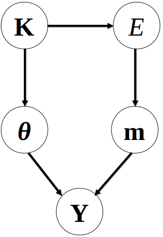
In the perspective of change-point comparison, we introduce the following event:

We further denote ${E}_{1}$ its complementary and define the binary random variable

The complete hierarchical model is displayed in Figure 1 and is defined as follows:

• •

  The random variable ${E}$ is drawn conditionally on ${\mathbf{K}}$ as a Bernoulli $\mathcal{B}(1-p_{0}({\mathbf{K}}))$ where $p_{0}({\mathbf{K}})=P({E}_{0}|{\mathbf{K}})$;

• •

  The parameters $\theta$ are drawn independently according to $P(\text{{$\theta$}}|{\mathbf{K}})$;

• •

  The partitions are drawn conditionally on ${E}$ according to $P({\bf m}|{\mathbf{K}},{E})$;

• •

  The observations are generated according to the conditional distribution $P({\bf Y}|{\bf m},\text{{$\theta$}})$.

More specifically, denoting ${\mathcal{M}}_{{\mathbf{K}}}^{1,n+1}=\bigotimes_{\ell}{\mathcal{M}}_{K^{\ell}}^{1,n+1}$, the partitions are assumed to be uniformly distributed, conditional on $E$, that is

We propose to assess the existence of a common change-point location between the $I$ profiles based on the posterior probability of this event, namely $P({E}_{0}|{\bf Y},{\mathbf{K}}).$

The Bayes factor is sometimes preferred for model comparison; it can be computed exactly in a similar way:

We designed a simulation study to identify the influence of various parameters on the performances of our approach. The design is illustrated in Figure 2: we compared $3$ independent profiles with $7$ segments, with all odd (respectively even) segments sharing the same distribution. The first two profiles have identical segmentation $m$ given by $m=(1,101,201,301,401,501,601,701)$ and the change-point locations of the third one are progressively shifted apart as $\tau_{k}^{3}=\tau_{k}^{1}+2^{k-1}$, for each $1\leq k\leq 6$. We shall denote $d_{k}=\tau_{k}^{3}-\tau_{k}^{1}$ and drop the index $k$ when there is no ambiguity on it.

Our purpose is to mimic data obtained by RNA-Seq experiments, so that the parameters for the negative binomial distribution were chosen to fit typical real-data. Considering the model where odd segments are sampled with distribution ${\mathcal{N}B}(p_{0},\phi)$, and even with ${\mathcal{N}B}(p_{1},\phi)$, we chose two different values of $p_{0}$, $0.8$ and $0.5$, and for each of them, we made $p_{1}$ vary so that the odd-ratio $s:=p_{1}/(1-p_{1})/[p_{0}/(1-p_{0})]$ is $4$, $8$ and $16$. Finally, we used different values of $\phi$ as detailed in Table 1 in order to explore a wide range of possible dispersions while keeping a signal/noise ratio not too high. Note that the higher $\phi$, the less overdispersed the signal. From our experience, the configuration of parameter combinations with $p_{0}=0.5$ is the more typical of observed values for RNA-Seq data.

Provided that the ratio $\lambda=\phi(1-p)/p$ remains constant, the negative binomial distribution with dispersion parameter $\phi$ going to infinity converges to the Poisson distribution $\mathcal{P}(\lambda)$. We propose an identical simulation study based on the Poisson distribution for the comparison with non-dispersed datasets. Specifically, we used for $\lambda_{0}$ the values $1.25$ and $0.73$ so that the odd-ratios $s=4;8;16$ corresponded to the respective values $\lambda_{1}=5;10;20$ and $2.92;5.83;11.7$

In practice there is little chance that the overdispersion is known. We propose to estimate this parameter from the data and use the obtained value in the analysis. The results presented here used the estimator inspired from Johnson et al. (2005): starting from sliding window of size $15$, we compute the method of moments estimator of $\phi$, using the formula $\phi={E}^{2}(X)/(V(X)-{E}(X))$, and retain the median over all windows. When this median is negative (which is likely to happen in datasets with many zeros), we double the size of the window. In practice however, results are very similar when using maximum likelihood or quasi-maximum likelihood estimators on sliding windows.

We compute the posterior probability $P({E}_{0}|{\bf Y},{\mathbf{K}})$ for each simulation and each value of $d$. Figures 7 to 9 in Appendix A represent the boxplots of this probability for each configuration. For sake of visibility, the outliers were not drawn in those figures. Note that in each figure, the first boxplot corresponds to $d=0$ and thus to model ${E}_{0}$, while $d\neq 0$ for left boxplots so that the true model is ${E}_{1}$. These plots can be understood as abacus for the detection power of the proposed approach. For example, the perfect scenario corresponds to $s=16$ in the Poisson case of Figure 7.

As expected, these results show that the lower the value of $\phi$ (the Poisson distribution is interpreted here as $\phi=+\infty$), the most difficult the decision becomes. The trend is identical for decreasing values of the odd-ratio $s$ and decreasing values of $d$. In the most difficult scenario of very high dispersion compared to signal value, the method fails to provide satisfying decisions whatever the level of odd-ratio or distance between change-points. However, in most configurations, the method is adequate as soon as $d\geq 16$.

An important question is the impact of the estimation of the dispersion parameter. Interestingly, in the simulation study with $p_{0}=0.8$, our estimator tended to under-estimate $\phi$ (and thus over-estimate the dispersion) while it was the contrary in the simulation study with $p_{0}=0.5$. This affects the performance of the decision rule, which behaves better when $\phi$ is higher. For instance, Figure 3 shows, for $s=16$ and $d=16$, that knowing the true value of $\phi$ improves the results when $p_{0}=0.8$ but worsens them when $p_{0}=0.5$.

References

- Bai and Perron [2003] J. Bai and P. Perron. Computation and analysis of multiple structural change models. J. Appl. Econ., 18:1–22, 2003.
- Dobigeon et al. [2007] Nicolas Dobigeon, Jean-Yves Tourneret, and Jeffrey D Scargle. Joint segmentation of multivariate astronomical time series: Bayesian sampling with a hierarchical model. Signal Processing, IEEE Transactions on, 55(2):414–423, 2007.
- Ehsanzadeh et al. [2011] Eghbal Ehsanzadeh, Taha BMJ Ouarda, and Hadiza M Saley. A simultaneous analysis of gradual and abrupt changes in Canadian low streamflows. Hydrological Processes, 25(5):727–739, 2011.
- Feder [1975] Paul I. Feder. The log likelihood ratio in segmented regression. Ann. Stat., 3:84–97, 1975. .
- Hušková and Kirch [2008] Marie Hušková and Claudia Kirch. Bootstrapping confidence intervals for the change-point of time series. Journal of Time Series Analysis, 29(6):947–972, 2008. ISSN 1467-9892. . URL http://dx.doi.org/10.1111/j.1467-9892.2008.00589.x.
- Johnson et al. [2005] N. Johnson, A.W. Kemp, and S. Kotz. Univariate discrete distributions. John Wiley & Sons, Inc., 2005.
- Mandal et al. [2004] Subhrangsu S Mandal, Chun Chu, Tadashi Wada, Hiroshi Handa, Aaron J Shatkin, and Danny Reinberg. Functional interactions of RNA-capping enzyme with factors that positively and negatively regulate promoter escape by RNA polymerase II. Proc Natl Acad Sci U S A, 101(20):7572–7, 2004.
- Muggeo [2003] V. M. Muggeo. Estimating regression models with unknown break-points. Stat Med, 22:3055–3071, 2003.
- Picard et al. [2011] Franck Picard, Emilie Lebarbier, Mark Hoebeke, Guillem Rigaill, Baba Thiam, and Stéphane Robin. Joint segmentation, calling, and normalization of multiple CGH profiles. Biostatistics, 12(3):413–428, 2011.
- Proudfoot et al. [2002] Nick Proudfoot, Andre Furger, and Michael Dye. Integrating mRNA processing with transcription. Cell, 108:501–512, 2002.
- Rand [1971] William M Rand. Objective criteria for the evaluation of clustering methods. Journal of the American Statistical association, 66(336):846–850, 1971.
- Reeves et al. [2007] J. Reeves, J. Chen, X. L. Wang, R. Lund, and L. QiQi. A review and comparison of changepoint detection techniques for climate data. Journal of Applied Meteorology and Climatology, 46(6):900–915, 2007.
- Rigaill et al. [2012] G. Rigaill, E. Lebarbier, and S. Robin. Exact posterior distributions and model selection criteria for multiple change-point detection problems. Statistics and Computing, 22:917–929, 2012. ISSN 0960-3174.
- Risso et al. [2011] Davide Risso, Katja Schwartz, Gavin Sherlock, and Sandrine Dudoit. GC-content normalization for RNA-Seq data. BMC Bioinformatics, 12(1):480, 2011.
- Tian et al. [2005] Bin Tian, Jun Hu, Haibo Zhang, and Carol Lutz. A large-scale analysis of mRNA polyadenylation of human and mouse genes. Nucleic Acids Research, 33:201–212, 2005.
- Toms and Lesperance [2003] J.D. Toms and M.L. Lesperance. Piecewise regression: A tool for identifying ecological thresholds. Ecology, 84(8):2034–41, 2003.
A Appendix section