跳到论文正文
W Papers独立论文阅读器 arXiv:1307.2798 论文正文 计算阅读时间 · 0%
引用这篇论文根据当前论文元数据生成,正式投稿前建议核对。


License: arXiv.org perpetual non-exclusive license
arXiv:1307.2798v1 [q-bio.NC] 10 Jul 2013

Correlation structure of stochastic neural networks with generic connectivity matrices

Diego Fasoli*    Olivier Faugeras*

*NeuroMathComp Laboratory, INRIA Sophia-Antipolis, France. Email: firstname.name@inria.fr

Abstract

Using a perturbative expansion for weak synaptic weights and weak sources of randomness, we calculate the correlation structure of neural networks with generic connectivity matrices.

In detail, the perturbative parameters are the mean and the standard deviation of the synaptic weights, together with the standard deviations of the background noise of the membrane potentials and of their initial conditions.

We also show how to determine the correlation structure of the system when the synaptic connections have a random topology.

This analysis is performed on rate neurons described by Wilson and Cowan equations, since this allows us to find analytic results.

Moreover, the perturbative expansion can be developed at any order and for a generic connectivity matrix.

We finally show an example of application of this technique for a particular case of biologically relevant topology of the synaptic connections.

1 Introduction

The brain is a system characterized by extremely high levels of complexity, which is inherited from the intricate network of its synaptic connections, known as connectome.

Therefore it seems plausible to attribute to the connectivity structure the incredible information processing capabilities of the brain.

As a consequence of this point of view, an increasing effort has been devoted to determining the connectome of different animal species.

In particular it has been already completed for the C. elegans [1][2], and partially determined for the mouse [3][4][5], the rat [6][7], the cat [8][9] and the monkey [10].

Recently the project has been started also for humans [11][12][13].

Some topological features of these networks of connections are already known, and the most notable are their small world properties and the presence of nested structures.

The small world topology refers to the fact that even if most nodes are not connected to the others, namely even if the network is not fully connected, they can be reached from the other nodes traveling along a small number of connections.

Networks with this kind of connectivity show enhanced information processing capabilities, wiring costs, speed of propagation of the signals and synchronizability, as discussed by many authors [14][15][16].

But the brain is also characterized by a nested structure of the synaptic connections, namely by different scales of organization.

In fact at the largest scale the brain can be seen as a single and highly complex macroscopic system, which is able to perform a series of differentiated tasks like learning, face recognition, reasoning, speech, movement coordination, and so on.

Then the brain can be decomposed into many sub-regions with specific purposes, like the cerebral cortex, the cerebellum, the hippocampus, the brain stem, etc.

Moreover, each one of these sub-regions can be divided further into other smaller areas with more specialized functions.

For example, wide parts of the cerebral cortex are involved in the reception of images, smells, sounds, flavors or pain and temperature.

These areas are known respectively as visual, olfactory, auditory, gustatory and somatosensory cortices.

If now for instance we take into account the visual cortex, we can decompose it in even smaller parts specialized in the detection of all the features of an image, like color, shadow, boundaries, orientations, and so on.

However all these regions of the brain are still characterized by a macroscopic scale.

Then we can go deeper and deeper in the subdivision process, until we reach the mesoscopic scale, which is marked by the presence of cortical columns [17].

These columns are in turn formed by many interconnected populations of neurons known as neural masses [18], from which we can finally go down to the lowest level, namely the microscopic scale of single neurons.

Moving from the macroscopic to the microscopic scale, the density of the synaptic connections increases, therefore they actually form a nested structure.

According to Sporns [19], this topology can be approximated by a fractal connectivity matrix, with a tunable level of complexity.

This represents a considerable improvement in the modelization of biologically realistic networks.

In particular, it is of extreme importance to determine the functional and information processing capabilities that emerge from this nested structure.

From this point of view, the first and simplest step is to determine the relation between the pattern of the synaptic connections, known as structural or anatomical connectivity, and the corresponding correlation structure of the neurons, known as functional connectivity.

Recently this problem has received the attention of the scientific community [20][21][22][23][24][25].

However, from a theoretical point of view, the calculation of the correlation structure of the system is not an easy problem, especially for highly complex connectivity matrices.

This analysis has been performed for relatively simple synaptic topologies, like fully connected networks [26][27] and connections with special kinds of invariance [28].

In this article we develop a perturbative approach that allows us to determine the correlation structure of the system for every possible topology of the synaptic connections, provided that the synaptic weights are weak enough.

In particular, we show how to apply this technique to the case of the fractal connectivity matrix introduced by Sporns.

2 Description of the model

The perturbative approach developed in this article can be applied to any neural model, but we take into account only the case of rate neurons described by Wilson and Cowan equations [26][28][29][30][31][32], because for this kind of neural equations the perturbative method provides analytic results. So we suppose that the neural network is described by the following system of stochastic differential equations:

d​Vi​(t)=[−1τ​Vi​(t)+∑j=0N−1Ji​j​(t)​S​(Vj​(t))+Ii​(t)]​d​t+σ1​d​Bi​(t)dV_{i}\left(t\right)=\left[-\frac{1}{\tau}V_{i}\left(t\right)+\sum_{j=0}^{N-1}J_{ij}\left(t\right)S\left(V_{j}\left(t\right)\right)+I_{i}\left(t\right)\right]dt+\sigma_{1}dB_{i}\left(t\right) (2.1)

with i=0,1,…,N−1i=0,1,...,N-1, where:

  • —

    NN is the number of neurons in the network;

  • —

    Vi​(t)V_{i}\left(t\right) is the membrane potential of the ii-th neuron;

  • —

    τ\tau is a time constant that describes the speed of convergence to a stationary state;

  • —

    Ii​(t)I_{i}\left(t\right) is the deterministic external input current of the ii-th neuron;

  • —

    Bi​(t)B_{i}\left(t\right) is the Brownian motion that describes the background noise of the ii-th neuron (or equivalently the stochastic part of the external input current);

  • —

    σ1\sigma_{1} is the standard deviation of the Brownian motions, which for simplicity is supposed to be the same for all the neurons and time-independent;

  • —

    Ji​j​(t)J_{ij}\left(t\right) is the random synaptic weight from the jj-th neuron to the ii-th neuron;

  • —

    S⁡(⋅)S\left(\cdot\right) is an activation function that converts the membrane potential of a neuron into the rate or frequency of the spikes it generates.

Usually in neuroscience S⁡(⋅)S\left(\cdot\right) is a sigmoid function, defined as:

S⁡(V)=TM​A​X1+e−λ⁡(V−VT)S\left(V\right)=\frac{T_{MAX}}{1+e^{-\lambda\left(V-V_{T}\right)}} (2.2)

where TM​A​XT_{MAX} is the maximum amplitude of the function (which is reached for V→+∞V\rightarrow+\infty), λ\lambda is the parameter that determine its slope for TM​A​XT_{MAX} fixed, while VTV_{T} represents the horizontal shift of the function along the VV axis.

Randomness is present in the system through three different variables, the Brownian motions, the initial conditions and the strength of the synaptic weights, which are treated perturbatively. Their distributions are supposed to be normal, because this allows us to calculate analytically the correlation structure of the network using the Isserlis’ theorem [33]. We also introduce a fourth non-perturbative source of randomness, namely the topology of the synaptic connections. This means that not only the intensities of the synaptic weights are considered as random, but also the existence or not of a connection between two given neurons is not certain anymore. For the first three variables, we use the same covariance structures as in [28]. For the Brownian motions it is given by the matrix Σ1\Sigma_{1}, whose entries are:

[Σ1]i​j=\displaystyle\left[\Sigma_{1}\right]_{ij}= C​o​v​(d​Bi​(t)d​t,d​Bj​(s)d​s)=Ci​j1​δ​(t−s)\displaystyle Cov\left(\frac{dB_{i}\left(t\right)}{dt},\frac{dB_{j}\left(s\right)}{ds}\right)=C_{ij}^{1}\delta\left(t-s\right)
Ci​j1=\displaystyle C_{ij}^{1}= {1ifi=jC1ifi≠j\displaystyle\begin{cases}1&\begin{array}[]{ccc}\mathrm{if}&&i=j\end{array}\\ \\ C_{1}&\begin{array}[]{ccc}\mathrm{if}&&i\neq j\end{array}\end{cases}

where C1C_{1} is a free parameter that represents the correlation between two Brownian motions, while δ⁡(⋅)\delta\left(\cdot\right) is the Dirac delta function. The matrix Σ1\Sigma_{1} is a genuine covariance matrix only if it is positive-semidefinite, namely if 11−N≤C1≤1\frac{1}{1-N}\leq C_{1}\leq 1.

The initial conditions are defined in terms of the following multivariate normal process:

V→​(0)∼𝒩⁡(μ→,Σ2)\overrightarrow{V}\left(0\right)\sim\mathcal{N}\left(\overrightarrow{\mu},\Sigma_{2}\right) (2.4)

where:

Σ2=σ22​[1C2⋯C2C21⋯C2⋮⋮⋱⋮C2C2⋯1]\Sigma_{2}=\sigma_{2}^{2}\left[\begin{array}[]{cccc}1&C_{2}&\cdots&C_{2}\\ C_{2}&1&\cdots&C_{2}\\ \vdots&\vdots&\ddots&\vdots\\ C_{2}&C_{2}&\cdots&1\end{array}\right] (2.5)

The parameter σ2\sigma_{2} represents the standard deviation of the initial conditions, while C2C_{2} is their correlation. Again we have to choose 11−N≤C2≤1\frac{1}{1-N}\leq C_{2}\leq 1.

In this article we consider networks with random topologies, which means that the fact to have or not a connection between two given neurons is a (known) random variable: if in one realization of the network there is a connection from the jj-th neuron to the ii-th neuron, in another realization this connection could be missing. Therefore we suppose that the synaptic weights are given by the following formulae:

Ji​j​(t)=\displaystyle J_{ij}\left(t\right)= {1Mi​[σ4​J¯i​j​(t)+σ3​Wi​j]ifMi≠00ifMi=0\displaystyle\begin{cases}\frac{1}{M_{i}}\left[\sigma_{4}\overline{J}_{ij}\left(t\right)+\sigma_{3}W_{ij}\right]&\begin{array}[]{ccc}\mathrm{if}&&M_{i}\neq 0\end{array}\\ \\ 0&\begin{array}[]{ccc}\mathrm{if}&&M_{i}=0\end{array}\end{cases} (2.6)
J¯i​j​(t)=\displaystyle\overline{J}_{ij}\left(t\right)= J¯^i​j​(t)∘T\displaystyle\widehat{\overline{J}}_{ij}\left(t\right)\circ T (2.7)
W=\displaystyle W= W^∘T\displaystyle\widehat{W}\circ T (2.8)
W^∼\displaystyle\widehat{W}\sim ℳ​𝒩​(0,Ω3,Σ3)\displaystyle\mathcal{MN}\left(0,\Omega_{3},\Sigma_{3}\right) (2.9)
Mi=\displaystyle M_{i}= ∑j=0N−1Ti​j\displaystyle\sum_{j=0}^{N-1}T_{ij} (2.10)

where σ3\sigma_{3} and σ4\sigma_{4} are two perturbative parameters that represent (after the division by MiM_{i}), respectively, the standard deviation and the mean strength of the synaptic connections. MiM_{i} is the number (in general random) of incoming connections to the ii-th neuron, and is used to prevent the explosion of the term ∑j=0N−1Ji​j​(t)​S​(Vj​(t)){\displaystyle\sum_{j=0}^{N-1}}J_{ij}\left(t\right)S\left(V_{j}\left(t\right)\right) in equation 2.1 when MiM_{i} grows arbitrarily large. The symbol “∘\circ” represents the Hadamard product, therefore C=A∘BC=A\circ B means that Ci​j=Ai​j​Bi​jC_{ij}=A_{ij}B_{ij}, ∀i,j\forall i,j. TT is a generic binary random matrix which represents the topology of the synaptic connections. More explicitly, we have Ti​j=0T_{ij}=0 if there is no connection from the jj-th to the ii-th neuron (namely if Ji​j​(t)=0J_{ij}\left(t\right)=0 ∀t\forall t), while Ti​j=1T_{ij}=1 if this connection is present. Below we show an example of connectivity matrix and its corresponding topology:

J¯​(t)=[002​c​o​s​(t)3.6s​i​n​(5​t)01001π0a​r​c​t​a​n​(7​t)0(1+t)−5e−3​t0],T=[0011101011010110]\begin{array}[]{ccc}\overline{J}\left(t\right)=\left[\begin{array}[]{cccc}0&0&2cos\left(t\right)&3.6\\ sin\left(5t\right)&0&10&0\\ 1&\pi&0&arctan\left(7t\right)\\ 0&\left(1+t\right)^{-5}&e^{-3t}&0\end{array}\right],&&T=\left[\begin{array}[]{cccc}0&0&1&1\\ 1&0&1&0\\ 1&1&0&1\\ 0&1&1&0\end{array}\right]\end{array}

The matrix J¯^​(t)\hat{\overline{J}}\left(t\right) is completely deterministic, while the matrix W^\widehat{W} is random only in the amplitudes of the synaptic weights (which follow a matrix normal distribution ℳ​𝒩​(0,Ω3,Σ3)\mathcal{MN}\left(0,\Omega_{3},\Sigma_{3}\right) [34]), but not in the topology. The covariance matrices Ω3\Omega_{3} and Σ3\Sigma_{3} of W^\widehat{W} are chosen in order to have:

C​o​v​(W^i​j,W^k​l)={1if(i=k)∧(j=l)C3otherwiseCov\left(\widehat{W}_{ij},\widehat{W}_{kl}\right)=\begin{cases}1&\begin{array}[]{ccc}\mathrm{if}&&\left(i=k\right)\wedge\left(j=l\right)\end{array}\\ \\ C_{3}&\mathrm{otherwise}\end{cases} (2.11)

The free parameter C3C_{3} represents the correlation between two different and non-zero synaptic weights, and the range of its plausible values depends on the topology of the connections, which is supposed to be completely generic. Moreover we assume that W^\widehat{W} and TT are independent.

To finish, we suppose that also the Brownian motions, the initial conditions, the amplitudes of the synaptic weights and the topology are independent from each other, therefore their reciprocal covariances are equal to zero:

C​o​v​(Bi​(t),Vj​(0))=C​o​v​(Bi​(t),W^j​k)=C​o​v​(Bi​(t),Tj​k)\displaystyle Cov\left(B_{i}\left(t\right),V_{j}\left(0\right)\right)=Cov\left(B_{i}\left(t\right),\widehat{W}_{jk}\right)=Cov\left(B_{i}\left(t\right),T_{jk}\right)
=C​o​v​(Vi​(0),W^j​k)=C​o​v​(Vi​(0),Tj​k)=0,∀i,j,k\displaystyle=Cov\left(V_{i}\left(0\right),\widehat{W}_{jk}\right)=Cov\left(V_{i}\left(0\right),T_{jk}\right)=0,\begin{array}[]{cc}&\forall i,j,k\end{array}

In principle, the inner and mutual covariance structure of Bi​(t)B_{i}\left(t\right), Vi​(0)V_{i}\left(0\right) and W^i​j\widehat{W}_{ij} can be arbitrarily chosen. However here we use only the simple structure defined by formulae , 2.5, 2.11 and 2, because this will generate simple analytic results for the correlation structure of the membrane potentials.

We now are ready to introduce a perturbative expansion of Vi​(t)V_{i}\left(t\right) in terms of the parameters σ\sigma:

Vi​(t)≈Y0i​(t)+∑m=14σm​Ymi​(t)+∑m,n=1m≤n4σm​σn​Ym,ni​(t)V_{i}\left(t\right)\approx Y_{0}^{i}\left(t\right)+\sum_{m=1}^{4}\sigma_{m}Y_{m}^{i}\left(t\right)+{\displaystyle\sum\limits_{\begin{subarray}{c}m,n=1\\ m\leq n\end{subarray}}^{4}}\sigma_{m}\sigma_{n}Y_{m,n}^{i}\left(t\right) (2.13)

where the functions Ymi​(t)Y_{m}^{i}\left(t\right) and Ym,ni​(t)Y_{m,n}^{i}\left(t\right) are to be determined through equation 2.1. In principle this expansion can be extended to any perturbative order, but in this article we truncate it at the second because the complexity of the results becomes quickly intractable.

2.1 The system of equations

In order to evaluate the functions Ymi​(t)Y_{m}^{i}\left(t\right) and Ym,ni​(t)Y_{m,n}^{i}\left(t\right), we have to replace the expansion 2.13 inside the equation 2.1, and to identify the coefficients of the same monomials in σ\sigma. Before doing this, we need the expansion of the sigmoid function in terms of σ\sigma. Therefore, defining:

ζj=∑m=14σm​Ymj​(t)+∑m,n=1m≤n4σm​σn​Ym,nj​(t)\zeta_{j}=\sum_{m=1}^{4}\sigma_{m}Y_{m}^{j}\left(t\right)+{\displaystyle\sum\limits_{\begin{subarray}{c}m,n=1\\ m\leq n\end{subarray}}^{4}}\sigma_{m}\sigma_{n}Y_{m,n}^{j}\left(t\right)

the Taylor expansion of the sigmoid function is:

S⁡(μ+ζj)≈\displaystyle S\left(\mu+\zeta_{j}\right)\approx S⁡(μ)+S′​(μ)​ζj+12​S′′​(μ)​ζj2\displaystyle S\left(\mu\right)+S^{\prime}\left(\mu\right)\zeta_{j}+\frac{1}{2}S^{\prime\prime}\left(\mu\right)\zeta_{j}^{2}
≈\displaystyle\approx S⁡(μ)+S′​(μ)​∑m=14σm​Ymj​(t)\displaystyle S\left(\mu\right)+S^{\prime}\left(\mu\right)\sum_{m=1}^{4}\sigma_{m}Y_{m}^{j}\left(t\right)
+∑m,n=1m<n4σmσn[S′(μ)Ym,nj(t)+S′′(μ)Ymj(t)Ynj(t)]\displaystyle+{\displaystyle\sum\limits_{\begin{subarray}{c}m,n=1\\ m<n\end{subarray}}^{4}}\sigma_{m}\sigma_{n}\left[S^{\prime}\left(\mu\right)Y_{m,n}^{j}\left(t\right)+S^{\prime\prime}\left(\mu\right)Y_{m}^{j}\left(t\right)Y_{n}^{j}\left(t\right)\right]
+∑m=14σm2[S′(μ)Ym,mj(t)+12S′′(μ)(Ymj(t))2]\displaystyle+\sum_{m=1}^{4}\sigma_{m}^{2}\left[S^{\prime}\left(\mu\right)Y_{m,m}^{j}\left(t\right)+\frac{1}{2}S^{\prime\prime}\left(\mu\right)\left(Y_{m}^{j}\left(t\right)\right)^{2}\right]

having neglected the terms with order higher than 22. This expansion can be used provided that its radius of convergence is large enough. The rigorous analysis can be found in [28] and shows that the expansion is convergent if the sigmoid function is not too steep at V=VTV=V_{T}, namely if the parameter λ\lambda is not too large. Now, if we replace this expansion and 2.13 inside the equation 2.1, comparing the coefficients of the same monomials in σ\sigma we obtain the following equations:

d​Y0i​(t)=\displaystyle dY_{0}^{i}\left(t\right)= [−1τ​Y0i​(t)+Ii​(t)]​d​t\displaystyle\left[-\frac{1}{\tau}Y_{0}^{i}\left(t\right)+I_{i}\left(t\right)\right]dt (2.14)
d​Y1i​(t)=\displaystyle dY_{1}^{i}\left(t\right)= −1τ​Y1i​(t)​d​t+d​Bi​(t)\displaystyle-\frac{1}{\tau}Y_{1}^{i}\left(t\right)dt+dB_{i}\left(t\right) (2.15)
d​Y2i​(t)=\displaystyle dY_{2}^{i}\left(t\right)= −1τ​Y2i​(t)​d​t\displaystyle-\frac{1}{\tau}Y_{2}^{i}\left(t\right)dt (2.16)
d​Y3i​(t)=\displaystyle dY_{3}^{i}\left(t\right)= [−1τ​Y3i​(t)+1Mi​∑j=0N−1Wi​j​S​(Y0j​(t))]​d​t\displaystyle\left[-\frac{1}{\tau}Y_{3}^{i}\left(t\right)+\frac{1}{M_{i}}\sum_{j=0}^{N-1}W_{ij}S\left(Y_{0}^{j}\left(t\right)\right)\right]dt (2.17)
d​Y4i​(t)=\displaystyle dY_{4}^{i}\left(t\right)= [−1τ​Y4i​(t)+1Mi​∑j=0N−1J¯i​j​(t)​S​(Y0j​(t))]​d​t\displaystyle\left[-\frac{1}{\tau}Y_{4}^{i}\left(t\right)+\frac{1}{M_{i}}\sum_{j=0}^{N-1}\overline{J}_{ij}\left(t\right)S\left(Y_{0}^{j}\left(t\right)\right)\right]dt (2.18)
d​Y1,4i​(t)=\displaystyle dY_{1,4}^{i}\left(t\right)= [−1τ​Y1,4i​(t)+1Mi​∑j=0N−1J¯i​j​(t)​S′​(Y0j​(t))​Y1j​(t)]​d​t\displaystyle\left[-\frac{1}{\tau}Y_{1,4}^{i}\left(t\right)+\frac{1}{M_{i}}\sum_{j=0}^{N-1}\overline{J}_{ij}\left(t\right)S^{\prime}\left(Y_{0}^{j}\left(t\right)\right)Y_{1}^{j}\left(t\right)\right]dt (2.19)
d​Y2,4i​(t)=\displaystyle dY_{2,4}^{i}\left(t\right)= [−1τ​Y2,4i​(t)+1Mi​∑j=0N−1J¯i​j​(t)​S′​(Y0j​(t))​Y2j​(t)]​d​t\displaystyle\left[-\frac{1}{\tau}Y_{2,4}^{i}\left(t\right)+\frac{1}{M_{i}}\sum_{j=0}^{N-1}\overline{J}_{ij}\left(t\right)S^{\prime}\left(Y_{0}^{j}\left(t\right)\right)Y_{2}^{j}\left(t\right)\right]dt (2.20)
d​Y3,4i​(t)=\displaystyle dY_{3,4}^{i}\left(t\right)= [−1τ​Y3,4i​(t)+1Mi​∑j=0N−1J¯i​j​(t)​S′​(Y0j​(t))​Y3j​(t)+1Mi​∑j=0N−1Wi​j​S′​(Y0j​(t))​Y4j​(t)]​d​t\displaystyle\left[-\frac{1}{\tau}Y_{3,4}^{i}\left(t\right)+\frac{1}{M_{i}}\sum_{j=0}^{N-1}\overline{J}_{ij}\left(t\right)S^{\prime}\left(Y_{0}^{j}\left(t\right)\right)Y_{3}^{j}\left(t\right)+\frac{1}{M_{i}}\sum_{j=0}^{N-1}W_{ij}S^{\prime}\left(Y_{0}^{j}\left(t\right)\right)Y_{4}^{j}\left(t\right)\right]dt (2.21)
d​Y4,4i​(t)=\displaystyle dY_{4,4}^{i}\left(t\right)= [−1τ​Y4,4i​(t)+1Mi​∑j=0N−1J¯i​j​(t)​S′​(Y0j​(t))​Y4j​(t)]​d​t\displaystyle\left[-\frac{1}{\tau}Y_{4,4}^{i}\left(t\right)+\frac{1}{M_{i}}\sum_{j=0}^{N-1}\overline{J}_{ij}\left(t\right)S^{\prime}\left(Y_{0}^{j}\left(t\right)\right)Y_{4}^{j}\left(t\right)\right]dt (2.22)

We have only written the equations that will be used in Section 3. The others do not influence the perturbative expansions of the variance and covariance truncated at the 33rd perturbative order, therefore they are not shown here.

2.2 The initial conditions

The perturbative expansion 2.13 at t=0t=0 gives:

Vi​(0)≈Y0i​(0)+∑m=14σm​Ymi​(0)+∑m,n=1m≤n4σm​σn​Ym,ni​(0)V_{i}\left(0\right)\approx Y_{0}^{i}\left(0\right)+\sum_{m=1}^{4}\sigma_{m}Y_{m}^{i}\left(0\right)+{\displaystyle\sum\limits_{\begin{subarray}{c}m,n=1\\ m\leq n\end{subarray}}^{4}}\sigma_{m}\sigma_{n}Y_{m,n}^{i}\left(0\right)

From 2.4 we have Vi​(0)∼𝒩⁡(μi,σ22)=μi+σ2​𝒩​(0,1)V_{i}\left(0\right)\sim\mathcal{N}\left(\mu_{i},\sigma_{2}^{2}\right)=\mu_{i}+\sigma_{2}\mathcal{N}\left(0,1\right), so comparing the two expressions we obtain:

Y0i​(0)=μi\displaystyle Y_{0}^{i}\left(0\right)=\mu_{i} (2.23)
Y2i​(0)∼𝒩⁡(0,1)\displaystyle Y_{2}^{i}\left(0\right)\sim\mathcal{N}\left(0,1\right) (2.24)
Ymi​(0)=0,m=1,3,4\displaystyle\begin{array}[]{ccc}Y_{m}^{i}\left(0\right)=0,&&m=1,3,4\end{array}
Ym,ni​(0)=0,∀(m,n):m≤n\displaystyle\begin{array}[]{ccc}Y_{m,n}^{i}\left(0\right)=0,&&\forall\left(m,n\right):\,m\leq n\end{array}

Therefore we can write the initial conditions as Vi​(0)=μi+σ2​Y2i​(0)V_{i}\left(0\right)=\mu_{i}+\sigma_{2}Y_{2}^{i}\left(0\right), from which we obtain:

C​o​v​(Vi​(0),Vj​(0))=σ22​C​o​v​(Y2i​(0),Y2j​(0))Cov\left(V_{i}\left(0\right),V_{j}\left(0\right)\right)=\sigma_{2}^{2}Cov\left(Y_{2}^{i}\left(0\right),Y_{2}^{j}\left(0\right)\right)

Since from 2.5 we also know that:

C​o​v​(Vi​(0),Vj​(0))={σ22ifi=jσ22​C2ifi≠jCov\left(V_{i}\left(0\right),V_{j}\left(0\right)\right)=\begin{cases}\sigma_{2}^{2}&\begin{array}[]{ccc}\mathrm{if}&&i=j\end{array}\\ \\ \sigma_{2}^{2}C_{2}&\begin{array}[]{ccc}\mathrm{if}&&i\neq j\end{array}\end{cases}

from the comparison of these two expressions of the covariance matrix of Vi​(0)V_{i}\left(0\right) we obtain:

C​o​v​(Y2i​(0),Y2j​(0))={1ifi=jC2ifi≠jCov\left(Y_{2}^{i}\left(0\right),Y_{2}^{j}\left(0\right)\right)=\begin{cases}1&\begin{array}[]{ccc}\mathrm{if}&&i=j\end{array}\\ \\ C_{2}&\begin{array}[]{ccc}\mathrm{if}&&i\neq j\end{array}\end{cases} (2.27)

2.3 Solutions of the equations

Since equations 2.14 - 2.22 are linear, they can be solved analytically, giving the following solutions:

Y0i​(t)=\displaystyle Y_{0}^{i}\left(t\right)= e−tτ​[μi+∫0tesτ​Ii​(s)​𝑑s]\displaystyle e^{-\frac{t}{\tau}}\left[\mu_{i}+\int_{0}^{t}e^{\frac{s}{\tau}}I_{i}\left(s\right)ds\right] (2.28)
Y1i​(t)=\displaystyle Y_{1}^{i}\left(t\right)= e−tτ​∫0tesτ​d​Bi​(s)\displaystyle e^{-\frac{t}{\tau}}\int_{0}^{t}e^{\frac{s}{\tau}}dB_{i}\left(s\right) (2.29)
Y2i​(t)=\displaystyle Y_{2}^{i}\left(t\right)= e−tτ​Y2i​(0)\displaystyle e^{-\frac{t}{\tau}}Y_{2}^{i}\left(0\right) (2.30)
Y3i​(t)=\displaystyle Y_{3}^{i}\left(t\right)= e−tτMi​∑j=0N−1Wi​j​∫0tesτ​S​(Y0j​(s))​𝑑s\displaystyle\frac{e^{-\frac{t}{\tau}}}{M_{i}}\sum_{j=0}^{N-1}W_{ij}\int_{0}^{t}e^{\frac{s}{\tau}}S\left(Y_{0}^{j}\left(s\right)\right)ds (2.31)
Y4i​(t)=\displaystyle Y_{4}^{i}\left(t\right)= e−tτMi​∑j=0N−1∫0tesτ​J¯i​j​(s)​S​(Y0j​(s))​𝑑s\displaystyle\frac{e^{-\frac{t}{\tau}}}{M_{i}}\sum_{j=0}^{N-1}\int_{0}^{t}e^{\frac{s}{\tau}}\overline{J}_{ij}\left(s\right)S\left(Y_{0}^{j}\left(s\right)\right)ds\hphantom{\,\,\,\,\,\,\,\,\,\,\,\,\,\,\,\,\,\,\,\,\,\,\,\,\,\,\,\,\,\,\,\,\,\,\,\,\,\,\,\,\,\,\,\,\,\,\,\,\,\,\,\,\,\,\,\,\,\,\,\,\,\,\,\,\,\,\,\,\,\,\,\,\,\,\,\,\,\,\,\,\,\,\,} (2.32)
Y1,4i​(t)=\displaystyle Y_{1,4}^{i}\left(t\right)= e−tτMi​∑j=0N−1∫0tJ¯i​j​(s)​S′​(Y0j​(s))​[∫0seuτ​d​Bj​(u)]​𝑑s\displaystyle\frac{e^{-\frac{t}{\tau}}}{M_{i}}\sum_{j=0}^{N-1}\int_{0}^{t}\overline{J}_{ij}\left(s\right)S^{\prime}\left(Y_{0}^{j}\left(s\right)\right)\left[\int_{0}^{s}e^{\frac{u}{\tau}}dB_{j}\left(u\right)\right]ds (2.33)
Y2,4i​(t)=\displaystyle Y_{2,4}^{i}\left(t\right)= e−tτMi​∑j=0N−1Y2j​(0)​∫0tJ¯i​j​(s)​S′​(Y0j​(s))​𝑑s\displaystyle\frac{e^{-\frac{t}{\tau}}}{M_{i}}\sum_{j=0}^{N-1}Y_{2}^{j}\left(0\right)\int_{0}^{t}\overline{J}_{ij}\left(s\right)S^{\prime}\left(Y_{0}^{j}\left(s\right)\right)ds (2.34)
Y3,4i​(t)=\displaystyle Y_{3,4}^{i}\left(t\right)= e−tτMi{∑j,k=0N−1Wj​kMj∫0tJ¯i​j(s)S′(Y0j(s))[∫0seuτS(Y0k(u))du]ds\displaystyle\frac{e^{-\frac{t}{\tau}}}{M_{i}}\left\{\sum_{j,k=0}^{N-1}\frac{W_{jk}}{M_{j}}\int_{0}^{t}\overline{J}_{ij}\left(s\right)S^{\prime}\left(Y_{0}^{j}\left(s\right)\right)\left[\int_{0}^{s}e^{\frac{u}{\tau}}S\left(Y_{0}^{k}\left(u\right)\right)du\right]ds\right.
+∑j,k=0N−1Wi​jMj∫0tS′(Y0j(s))[∫0seuτJ¯j​k(u)S(Y0k(u))du]ds}\displaystyle\left.+\sum_{j,k=0}^{N-1}\frac{W_{ij}}{M_{j}}\int_{0}^{t}S^{\prime}\left(Y_{0}^{j}\left(s\right)\right)\left[\int_{0}^{s}e^{\frac{u}{\tau}}\overline{J}_{jk}\left(u\right)S\left(Y_{0}^{k}\left(u\right)\right)du\right]ds\right\} (2.35)
Y4,4i​(t)=\displaystyle Y_{4,4}^{i}\left(t\right)= e−tτMi​∑j,k=0N−11Mj​∫0tJ¯i​j​(s)​S′​(Y0j​(s))​[∫0seuτ​J¯j​k​(u)​S​(Y0k​(u))​𝑑u]​𝑑s\displaystyle\frac{e^{-\frac{t}{\tau}}}{M_{i}}\sum_{j,k=0}^{N-1}\frac{1}{M_{j}}\int_{0}^{t}\overline{J}_{ij}\left(s\right)S^{\prime}\left(Y_{0}^{j}\left(s\right)\right)\left[\int_{0}^{s}e^{\frac{u}{\tau}}\overline{J}_{jk}\left(u\right)S\left(Y_{0}^{k}\left(u\right)\right)du\right]ds (2.36)

Now we can use these results to calculate the correlation structure of the membrane potentials.

3 Correlation structure of the network

In this section we analyze the general case of random topologies, and we consider the networks with deterministic connections as a special case. From the perturbative expansion 2.13 with all the functions Ymi​(t)Y_{m}^{i}\left(t\right) and Ym,ni​(t)Y_{m,n}^{i}\left(t\right) evaluated as shown in Section 2.3, in order to calculate the covariance matrix of the membrane potentials we need to determine all the pair covariances between all the possible combinations of these functions. This is a consequence of the bilinearity property of the covariance operator. However, using the Isserlis’ theorem and the relations 2, it is easy to see that many of these terms are equal to zero. Moreover we have also to remove the 44th order terms in the expression of the covariance, like σ12​σ32​C​o​v​(Y1,3i​(t),Y1,3j​(t))\sigma_{1}^{2}\sigma_{3}^{2}Cov\left(Y_{1,3}^{i}\left(t\right),Y_{1,3}^{j}\left(t\right)\right), since they are not complete. This is due to the fact that there are also 44th order terms like σ12​σ32​C​o​v​(Y1i​(t),Y1,1,3j​(t))\sigma_{1}^{2}\sigma_{3}^{2}Cov\left(Y_{1}^{i}\left(t\right),Y_{1,1,3}^{j}\left(t\right)\right). These terms are due to 33rd order functions, like Y1,1,3j​(t)Y_{1,1,3}^{j}\left(t\right) in this case, in the perturbative expansion 2.13, which have not been taken into account since we have truncated the expansion of the membrane potential at the 22nd order. Therefore the expansion of the covariance must be truncated at the 33rd order. So, to conclude, we obtain the following result:

C​o​v​(Vi​(t),Vj​(t))\displaystyle Cov\left(V_{i}\left(t\right),V_{j}\left(t\right)\right)
=σ12​C​o​v​(Y1i​(t),Y1j​(t))+σ22​C​o​v​(Y2i​(t),Y2j​(t))\displaystyle=\sigma_{1}^{2}Cov\left(Y_{1}^{i}\left(t\right),Y_{1}^{j}\left(t\right)\right)+\sigma_{2}^{2}Cov\left(Y_{2}^{i}\left(t\right),Y_{2}^{j}\left(t\right)\right)
+σ32​C​o​v​(Y3i​(t),Y3j​(t))+σ42​C​o​v​(Y4i​(t),Y4j​(t))\displaystyle+\sigma_{3}^{2}Cov\left(Y_{3}^{i}\left(t\right),Y_{3}^{j}\left(t\right)\right)+\sigma_{4}^{2}Cov\left(Y_{4}^{i}\left(t\right),Y_{4}^{j}\left(t\right)\right)
+σ4{σ12[Cov(Y1i(t),Y1,4j(t))+Cov(Y1,4i(t),Y1j(t))]+σ22[Cov(Y2i(t),Y2,4j(t))+Cov(Y2,4i(t),Y2j(t))]\displaystyle+\sigma_{4}\left\{\sigma_{1}^{2}\left[Cov\left(Y_{1}^{i}\left(t\right),Y_{1,4}^{j}\left(t\right)\right)+Cov\left(Y_{1,4}^{i}\left(t\right),Y_{1}^{j}\left(t\right)\right)\right]+\sigma_{2}^{2}\left[Cov\left(Y_{2}^{i}\left(t\right),Y_{2,4}^{j}\left(t\right)\right)+Cov\left(Y_{2,4}^{i}\left(t\right),Y_{2}^{j}\left(t\right)\right)\right]\right.
+σ32[Cov(Y3i(t),Y3,4j(t))+Cov(Y3,4i(t),Y3j(t))]+σ42[Cov(Y4i(t),Y4,4j(t))+Cov(Y4,4i(t),Y4j(t))]}\displaystyle\left.+\sigma_{3}^{2}\left[Cov\left(Y_{3}^{i}\left(t\right),Y_{3,4}^{j}\left(t\right)\right)+Cov\left(Y_{3,4}^{i}\left(t\right),Y_{3}^{j}\left(t\right)\right)\right]+\sigma_{4}^{2}\left[Cov\left(Y_{4}^{i}\left(t\right),Y_{4,4}^{j}\left(t\right)\right)+Cov\left(Y_{4,4}^{i}\left(t\right),Y_{4}^{j}\left(t\right)\right)\right]\right\}\hphantom{\,\,\,\,\,\,\,\,\,\,\,\,\,} (3.1)

where, due to formulae 2.29, 2.30 and 2.31, for i≠ji\neq j we obtain:

C​o​v​(Y1i​(t),Y1j​(t))=\displaystyle Cov\left(Y_{1}^{i}\left(t\right),Y_{1}^{j}\left(t\right)\right)= τ​C12​(1−e−2​tτ)\displaystyle\frac{\tau C_{1}}{2}\left(1-e^{-\frac{2t}{\tau}}\right) (3.2)
C​o​v​(Y2i​(t),Y2j​(t))=\displaystyle Cov\left(Y_{2}^{i}\left(t\right),Y_{2}^{j}\left(t\right)\right)= C2​e−2​tτ\displaystyle C_{2}e^{-\frac{2t}{\tau}} (3.3)
C​o​v​(Y3i​(t),Y3j​(t))=\displaystyle Cov\left(Y_{3}^{i}\left(t\right),Y_{3}^{j}\left(t\right)\right)= C3​e−2​tτ​∑k,l=0N−1[∫0tesτ​S​(Y0k​(s))​𝑑s]​[∫0tesτ​S​(Y0l​(s))​𝑑s]​𝔼​[Ti​k​Tj​lMi​Mj]\displaystyle C_{3}e^{-\frac{2t}{\tau}}{\displaystyle\sum\limits_{k,l=0}^{N-1}}\left[\int_{0}^{t}e^{\frac{s}{\tau}}S\left(Y_{0}^{k}\left(s\right)\right)ds\right]\left[\int_{0}^{t}e^{\frac{s}{\tau}}S\left(Y_{0}^{l}\left(s\right)\right)ds\right]\mathbb{E}\left[\frac{T_{ik}T_{jl}}{M_{i}M_{j}}\right] (3.4)

and for i=ji=j:

V​a​r​(Y1i​(t))=\displaystyle Var\left(Y_{1}^{i}\left(t\right)\right)= τ2​(1−e−2​tτ)\displaystyle\frac{\tau}{2}\left(1-e^{-\frac{2t}{\tau}}\right) (3.5)
V​a​r​(Y2i​(t))=\displaystyle Var\left(Y_{2}^{i}\left(t\right)\right)= e−2​tτ\displaystyle e^{-\frac{2t}{\tau}} (3.6)
V​a​r​(Y3i​(t))=\displaystyle Var\left(Y_{3}^{i}\left(t\right)\right)= e−2​tτ{∑k=0N−1[∫0tesτS(Y0k(s))ds]2𝔼[(Ti​kMi)2]\displaystyle e^{-\frac{2t}{\tau}}\left\{{\displaystyle\sum\limits_{k=0}^{N-1}}\left[\int_{0}^{t}e^{\frac{s}{\tau}}S\left(Y_{0}^{k}\left(s\right)\right)ds\right]^{2}\mathbb{E}\left[\left(\frac{T_{ik}}{M_{i}}\right)^{2}\right]\vphantom{{\displaystyle\sum\limits_{\begin{subarray}{c}k,l\\ k\neq l\end{subarray}}}}\right.
+C3∑k,lk≠l[∫0tesτS(Y0k(s))ds][∫0tesτS(Y0l(s))ds]𝔼[Ti​k​Ti​lMi2]}\displaystyle\left.+C_{3}{\displaystyle\sum\limits_{\begin{subarray}{c}k,l\\ k\neq l\end{subarray}}}\left[\int_{0}^{t}e^{\frac{s}{\tau}}S\left(Y_{0}^{k}\left(s\right)\right)ds\right]\left[\int_{0}^{t}e^{\frac{s}{\tau}}S\left(Y_{0}^{l}\left(s\right)\right)ds\right]\mathbb{E}\left[\frac{T_{ik}T_{il}}{M_{i}^{2}}\right]\right\}\hphantom{\,\,\,\,\,\,\,\,\,\,\,\,\,\,\,\,\,\,} (3.7)

Because of formulae 2.29 - 2.36, for all i,ji,j we obtain:

C​o​v​(Y4i​(t),Y4j​(t))=e−2​tτ​∑k,l=0N−1[∫0tesτ​J¯^i​k​(s)​S​(Y0k​(s))​𝑑s]​[∫0tesτ​J¯^j​l​(s)​S​(Y0l​(s))​𝑑s]​C​o​v​(Ti​kMi,Tj​lMj)\displaystyle Cov\left(Y_{4}^{i}\left(t\right),Y_{4}^{j}\left(t\right)\right)=e^{-\frac{2t}{\tau}}{\displaystyle\sum\limits_{k,l=0}^{N-1}}\left[\int_{0}^{t}e^{\frac{s}{\tau}}\hat{\overline{J}}_{ik}\left(s\right)S\left(Y_{0}^{k}\left(s\right)\right)ds\right]\left[\int_{0}^{t}e^{\frac{s}{\tau}}\hat{\overline{J}}_{jl}\left(s\right)S\left(Y_{0}^{l}\left(s\right)\right)ds\right]Cov\left(\frac{T_{ik}}{M_{i}},\frac{T_{jl}}{M_{j}}\right) (3.8)
C​o​v​(Y1i​(t),Y1,4j​(t))=\displaystyle Cov\left(Y_{1}^{i}\left(t\right),Y_{1,4}^{j}\left(t\right)\right)=
=τ2​e−2​tτ​{𝔼⁡[Tj​iMj]​[∫0tJ¯^j​i​(s)​S′​(Y0i​(s))​(e2​sτ−1)​𝑑s]+C1​∑k=0k≠iN−1𝔼⁡[Tj​kMj]​[∫0tJ¯^j​k​(s)​S′​(Y0k​(s))​(e2​sτ−1)​𝑑s]}\displaystyle=\frac{\tau}{2}e^{-\frac{2t}{\tau}}\left\{\mathbb{E}\left[\frac{T_{ji}}{M_{j}}\right]\left[\int_{0}^{t}\widehat{\overline{J}}_{ji}\left(s\right)S^{\prime}\left(Y_{0}^{i}\left(s\right)\right)\left(e^{\frac{2s}{\tau}}-1\right)ds\right]+C_{1}{\displaystyle\sum\limits_{\begin{subarray}{c}k=0\\ k\neq i\end{subarray}}^{N-1}}\mathbb{E}\left[\frac{T_{jk}}{M_{j}}\right]\left[\int_{0}^{t}\widehat{\overline{J}}_{jk}\left(s\right)S^{\prime}\left(Y_{0}^{k}\left(s\right)\right)\left(e^{\frac{2s}{\tau}}-1\right)ds\right]\right\} (3.9)
C​o​v​(Y2i​(t),Y2,4j​(t))=e−2​tτ​{𝔼⁡[Tj​iMj]​[∫0tJ¯^j​i​(s)​S​(Y0i​(s))​𝑑s]+C2​∑k=0k≠iN−1𝔼⁡[Tj​kMj]​[∫0tJ¯^j​k​(s)​S​(Y0k​(s))​𝑑s]}\displaystyle Cov\left(Y_{2}^{i}\left(t\right),Y_{2,4}^{j}\left(t\right)\right)=e^{-\frac{2t}{\tau}}\left\{\mathbb{E}\left[\frac{T_{ji}}{M_{j}}\right]\left[\int_{0}^{t}\widehat{\overline{J}}_{ji}\left(s\right)S\left(Y_{0}^{i}\left(s\right)\right)ds\right]+C_{2}{\displaystyle\sum\limits_{\begin{subarray}{c}k=0\\ k\neq i\end{subarray}}^{N-1}}\mathbb{E}\left[\frac{T_{jk}}{M_{j}}\right]\left[\int_{0}^{t}\widehat{\overline{J}}_{jk}\left(s\right)S\left(Y_{0}^{k}\left(s\right)\right)ds\right]\right\} (3.10)
C​o​v​(Y3i​(t),Y3,4j​(t))\displaystyle Cov\left(Y_{3}^{i}\left(t\right),Y_{3,4}^{j}\left(t\right)\right)
=e−2​tτ{∑k=0N−1𝔼[(Ti​kMi)2Tj​iMj][∫0tesτS(Y0k(s))ds]∫0tJ¯^j​i(s)S′(Y0i(s))[∫0seuτS(Y0k(u))du]ds\displaystyle=e^{-\frac{2t}{\tau}}\left\{{\displaystyle\sum\limits_{k=0}^{N-1}}\mathbb{E}\left[\left(\frac{T_{ik}}{M_{i}}\right)^{2}\frac{T_{ji}}{M_{j}}\right]\left[\int_{0}^{t}e^{\frac{s}{\tau}}S\left(Y_{0}^{k}\left(s\right)\right)ds\right]\int_{0}^{t}\widehat{\overline{J}}_{ji}\left(s\right)S^{\prime}\left(Y_{0}^{i}\left(s\right)\right)\left[\int_{0}^{s}e^{\frac{u}{\tau}}S\left(Y_{0}^{k}\left(u\right)\right)du\right]ds\right.
+C3∑k,l=0N−1𝔼[Ti​k​Ti​l​Tj​iMi2​Mj][∫0tesτS(Y0k(s))ds]∫0tJ¯^j​i(s)S′(Y0i(s))[∫0seuτS(Y0l(u))du]ds\displaystyle+C_{3}{\displaystyle\sum\limits_{k,l=0}^{N-1}}\mathbb{E}\left[\frac{T_{ik}T_{il}T_{ji}}{M_{i}^{2}M_{j}}\right]\left[\int_{0}^{t}e^{\frac{s}{\tau}}S\left(Y_{0}^{k}\left(s\right)\right)ds\right]\int_{0}^{t}\widehat{\overline{J}}_{ji}\left(s\right)S^{\prime}\left(Y_{0}^{i}\left(s\right)\right)\left[\int_{0}^{s}e^{\frac{u}{\tau}}S\left(Y_{0}^{l}\left(u\right)\right)du\right]ds
+C3∑k,l=0N−1𝔼[Ti​k​Tl​k​Tj​lMi​Mj​Ml][∫0tesτS(Y0k(s))ds]∫0tJ¯^j​l(s)S′(Y0l(s))[∫0seuτS(Y0k(u))du]ds\displaystyle+C_{3}{\displaystyle\sum\limits_{k,l=0}^{N-1}}\mathbb{E}\left[\frac{T_{ik}T_{lk}T_{jl}}{M_{i}M_{j}M_{l}}\right]\left[\int_{0}^{t}e^{\frac{s}{\tau}}S\left(Y_{0}^{k}\left(s\right)\right)ds\right]\int_{0}^{t}\widehat{\overline{J}}_{jl}\left(s\right)S^{\prime}\left(Y_{0}^{l}\left(s\right)\right)\left[\int_{0}^{s}e^{\frac{u}{\tau}}S\left(Y_{0}^{k}\left(u\right)\right)du\right]ds
+C3∑k,l,m=0N−1𝔼[Ti​k​Tl​m​Tj​lMi​Mj​Ml][∫0tesτS(Y0k(s))ds]∫0tJ¯^j​l(s)S′(Y0l(s))[∫0seuτS(Y0m(u))du]ds}\displaystyle\left.+C_{3}{\displaystyle\sum\limits_{k,l,m=0}^{N-1}}\mathbb{E}\left[\frac{T_{ik}T_{lm}T_{jl}}{M_{i}M_{j}M_{l}}\right]\left[\int_{0}^{t}e^{\frac{s}{\tau}}S\left(Y_{0}^{k}\left(s\right)\right)ds\right]\int_{0}^{t}\widehat{\overline{J}}_{jl}\left(s\right)S^{\prime}\left(Y_{0}^{l}\left(s\right)\right)\left[\int_{0}^{s}e^{\frac{u}{\tau}}S\left(Y_{0}^{m}\left(u\right)\right)du\right]ds\right\} (3.11)
C​o​v​(Y4i​(t),Y4,4j​(t))\displaystyle Cov\left(Y_{4}^{i}\left(t\right),Y_{4,4}^{j}\left(t\right)\right)
=e−2​tτ​∑k,l,m=0N−1C​o​v​(Ti​kMi,Tj​l​Tl​mMj​Ml)​[∫0tesτ​J¯^i​k​(s)​S​(Y0k​(s))​𝑑s]​[∫0tJ¯^j​l​(s)​S′​(Y0l​(s))​[∫0seuτ​J¯^l​m​(s)​S​(Y0m​(u))​𝑑u]​𝑑s]\displaystyle=e^{-\frac{2t}{\tau}}{\displaystyle\sum\limits_{k,l,m=0}^{N-1}}Cov\left(\frac{T_{ik}}{M_{i}},\frac{T_{jl}T_{lm}}{M_{j}M_{l}}\right)\left[\int_{0}^{t}e^{\frac{s}{\tau}}\widehat{\overline{J}}_{ik}\left(s\right)S\left(Y_{0}^{k}\left(s\right)\right)ds\right]\left[\int_{0}^{t}\widehat{\overline{J}}_{jl}\left(s\right)S^{\prime}\left(Y_{0}^{l}\left(s\right)\right)\left[\int_{0}^{s}e^{\frac{u}{\tau}}\widehat{\overline{J}}_{lm}\left(s\right)S\left(Y_{0}^{m}\left(u\right)\right)du\right]ds\right] (3.12)

Formula 3.9 is obtained using the following identity (which is a consequence of the mutual independence of the random variables):

C​o​v​(Bi​(t),Bj​(t)​J¯k​l​(t)Mk)=\displaystyle Cov\left(B_{i}\left(t\right),B_{j}\left(t\right)\frac{\overline{J}_{kl}\left(t\right)}{M_{k}}\right)= 𝔼⁡[Bi​(t)​Bj​(t)​J¯^k​l​(t)​Tk​lMk]−𝔼⁡[Bi​(t)]​𝔼​[Bj​(t)​J¯^k​l​(t)​Tk​lMk]\displaystyle\mathbb{E}\left[B_{i}\left(t\right)B_{j}\left(t\right)\widehat{\overline{J}}_{kl}\left(t\right)\frac{T_{kl}}{M_{k}}\right]-\mathbb{E}\left[B_{i}\left(t\right)\right]\mathbb{E}\left[B_{j}\left(t\right)\widehat{\overline{J}}_{kl}\left(t\right)\frac{T_{kl}}{M_{k}}\right]
=\displaystyle= J¯^k​l​(t)​(𝔼⁡[Bi​(t)​Bj​(t)]​𝔼​[Tk​lMk]−𝔼⁡[Bi​(t)]​𝔼​[Bj​(t)]​𝔼​[Tk​lMk])\displaystyle\widehat{\overline{J}}_{kl}\left(t\right)\left(\mathbb{E}\left[B_{i}\left(t\right)B_{j}\left(t\right)\right]\mathbb{E}\left[\frac{T_{kl}}{M_{k}}\right]-\mathbb{E}\left[B_{i}\left(t\right)\right]\mathbb{E}\left[B_{j}\left(t\right)\right]\mathbb{E}\left[\frac{T_{kl}}{M_{k}}\right]\right)
=\displaystyle= J¯^k​l​(t)​𝔼​[Tk​lMk]​C​o​v​(Bi​(t),Bj​(t))\displaystyle\widehat{\overline{J}}_{kl}\left(t\right)\mathbb{E}\left[\frac{T_{kl}}{M_{k}}\right]Cov\left(B_{i}\left(t\right),B_{j}\left(t\right)\right)

A similar relation can be found for the initial conditions V→​(0)\overrightarrow{V}\left(0\right) and the topology TT:

C​o​v​(Vi​(0),Vj​(0)​J¯k​l​(t)Mk)=J¯^k​l​(t)​𝔼​[Tk​lMk]​C​o​v​(Vi​(0),Vj​(0))Cov\left(V_{i}\left(0\right),V_{j}\left(0\right)\frac{\overline{J}_{kl}\left(t\right)}{M_{k}}\right)=\widehat{\overline{J}}_{kl}\left(t\right)\mathbb{E}\left[\frac{T_{kl}}{M_{k}}\right]Cov\left(V_{i}\left(0\right),V_{j}\left(0\right)\right)

from which we have obtained formula 3.10. Instead, in order to obtain formula 3.11, we have used the following result:

C​o​v​(Wi​jMi,Wk​lMk​J¯m​n​(t)Mm)=\displaystyle Cov\left(\frac{W_{ij}}{M_{i}},\frac{W_{kl}}{M_{k}}\frac{\overline{J}_{mn}\left(t\right)}{M_{m}}\right)= C​o​v​(W^i​j​Ti​jMi,W^k​l​Tk​lMk​J¯^m​n​(t)​Tm​nMm)\displaystyle Cov\left(\widehat{W}_{ij}\frac{T_{ij}}{M_{i}},\widehat{W}_{kl}\frac{T_{kl}}{M_{k}}\widehat{\overline{J}}_{mn}\left(t\right)\frac{T_{mn}}{M_{m}}\right)
=\displaystyle= J¯^m​n​(t)​(𝔼⁡[W^i​j​Ti​jMi​W^k​l​Tk​lMk​Tm​nMm]−𝔼⁡[W^i​j​Ti​jMi]​𝔼​[W^k​l​Tk​lMk​Tm​nMm])\displaystyle\widehat{\overline{J}}_{mn}\left(t\right)\left(\mathbb{E}\left[\widehat{W}_{ij}\frac{T_{ij}}{M_{i}}\widehat{W}_{kl}\frac{T_{kl}}{M_{k}}\frac{T_{mn}}{M_{m}}\right]-\mathbb{E}\left[\widehat{W}_{ij}\frac{T_{ij}}{M_{i}}\right]\mathbb{E}\left[\widehat{W}_{kl}\frac{T_{kl}}{M_{k}}\frac{T_{mn}}{M_{m}}\right]\right)
=\displaystyle= J¯^m​n​(t)​(𝔼⁡[W^i​j​W^k​l]​𝔼​[Ti​j​Tk​l​Tm​nMi​Mk​Mm]−𝔼⁡[W^i​j]​𝔼​[Ti​jMi]​𝔼​[W^k​l]​𝔼​[Tk​l​Tm​nMk​Mm])\displaystyle\widehat{\overline{J}}_{mn}\left(t\right)\left(\mathbb{E}\left[\widehat{W}_{ij}\widehat{W}_{kl}\right]\mathbb{E}\left[\frac{T_{ij}T_{kl}T_{mn}}{M_{i}M_{k}M_{m}}\right]-\mathbb{E}\left[\widehat{W}_{ij}\right]\mathbb{E}\left[\frac{T_{ij}}{M_{i}}\right]\mathbb{E}\left[\widehat{W}_{kl}\right]\mathbb{E}\left[\frac{T_{kl}T_{mn}}{M_{k}M_{m}}\right]\right)
=\displaystyle= J¯^m​n​(t)​C​o​v​(W^i​j,W^k​l)​𝔼​[Ti​j​Tk​l​Tm​nMi​Mk​Mm]\displaystyle\widehat{\overline{J}}_{mn}\left(t\right)Cov\left(\widehat{W}_{ij},\widehat{W}_{kl}\right)\mathbb{E}\left[\frac{T_{ij}T_{kl}T_{mn}}{M_{i}M_{k}M_{m}}\right]

which is a consequence of the independence between W^\widehat{W} and TT. In the same way it is possible to prove that:

C​o​v​(Wi​jMi,J¯k​l​(t)Mk​J¯m​n​(t)Mm)=J¯^k​l​(t)​J¯^m​n​(t)​𝔼​[W^i​j]​(𝔼⁡[Ti​j​Tk​l​Tm​nMi​Mk​Mm]−𝔼⁡[Ti​jMi]​𝔼​[Tk​l​Tm​nMk​Mm])=0Cov\left(\frac{W_{ij}}{M_{i}},\frac{\overline{J}_{kl}\left(t\right)}{M_{k}}\frac{\overline{J}_{mn}\left(t\right)}{M_{m}}\right)=\widehat{\overline{J}}_{kl}\left(t\right)\widehat{\overline{J}}_{mn}\left(t\right)\mathbb{E}\left[\widehat{W}_{ij}\right]\left(\mathbb{E}\left[\frac{T_{ij}T_{kl}T_{mn}}{M_{i}M_{k}M_{m}}\right]-\mathbb{E}\left[\frac{T_{ij}}{M_{i}}\right]\mathbb{E}\left[\frac{T_{kl}T_{mn}}{M_{k}M_{m}}\right]\right)=0

so for this reason the term C​o​v​(Y3i​(t),Y4,4i​(t))Cov\left(Y_{3}^{i}\left(t\right),Y_{4,4}^{i}\left(t\right)\right) does not appear in formula 3.1.

Once the covariance matrix of the membrane potentials has been determined, we can evaluate their correlation structure using the Pearson’s correlation coefficient, defined as follows:

C​o​r​r​(Vi​(t),Vj​(t))=C​o​v​(Vi​(t),Vj​(t))V​a​r​(Vi​(t))​V​a​r​(Vj​(t))Corr\left(V_{i}\left(t\right),V_{j}\left(t\right)\right)=\frac{Cov\left(V_{i}\left(t\right),V_{j}\left(t\right)\right)}{\sqrt{Var\left(V_{i}\left(t\right)\right)Var\left(V_{j}\left(t\right)\right)}} (3.13)

where:

V​a​r​(Vi​(t))=C​o​v​(Vi​(t),Vi​(t))Var\left(V_{i}\left(t\right)\right)=Cov\left(V_{i}\left(t\right),V_{i}\left(t\right)\right) (3.14)

is the variance of the stochastic process Vi​(t)V_{i}\left(t\right).

The only quantities that remain unspecified are 𝔼⁡[Ti​jMi]\mathbb{E}\left[\frac{T_{ij}}{M_{i}}\right], 𝔼⁡[Ti​k​Tj​lMi​Mj]\mathbb{E}\left[\frac{T_{ik}T_{jl}}{M_{i}M_{j}}\right] and 𝔼⁡[Ti​k​Tl​m​Tj​lMi​Mj​Ml]\mathbb{E}\left[\frac{T_{ik}T_{lm}T_{jl}}{M_{i}M_{j}M_{l}}\right], that depend on the distribution of the matrix TT. This can be accomplished by a multidimensional Taylor expansion. For example, for 𝔼⁡[Ti​jMi]\mathbb{E}\left[\frac{T_{ij}}{M_{i}}\right] we Taylor-expand the function:

f:(Ti​0,…,Ti,N−1)→Ti​jMi\begin{array}[]{cccc}f:&\left(T_{i0},...,T_{i,N-1}\right)&\rightarrow&\frac{T_{ij}}{M_{i}}\end{array} (3.15)

at the point (𝔼⁡[Ti​0],…,𝔼⁡[Ti,N−1])\left(\mathbb{E}\left[T_{i0}\right],...,\mathbb{E}\left[T_{i,N-1}\right]\right) to obtain:

𝔼⁡[Ti​jMi]=\displaystyle\mathbb{E}\left[\frac{T_{ij}}{M_{i}}\right]= 𝔼⁡[Ti​j∑k=0N−1Ti​k]\displaystyle\mathbb{E}\left[\frac{T_{ij}}{{\displaystyle\sum_{k=0}^{N-1}}T_{ik}}\right]
=\displaystyle= ∑n0=0∞∑n1=0∞⋯∑nN−1=0∞𝔼[(Ti​0−𝔼[Ti​0])n0⋯(Ti,N−1−𝔼[Ti,N−1])nN−1]n0!⋯nN−1!(∂n0+…+nN−1f∂Ti​0n0⋯∂Ti,N−1nN−1)(𝔼[Ti​0],⋯,𝔼[Ti,N−1])\displaystyle{\displaystyle{\displaystyle\sum_{n_{0}=0}^{\infty}}}{\displaystyle{\displaystyle\sum_{n_{1}=0}^{\infty}}}\cdots{\displaystyle{\displaystyle\sum_{n_{N-1}=0}^{\infty}}}\frac{\mathbb{E}\left[\left(T_{i0}-\mathbb{E}\left[T_{i0}\right]\right)^{n_{0}}\cdots\left(T_{i,N-1}-\mathbb{E}\left[T_{i,N-1}\right]\right)^{n_{N-1}}\right]}{n_{0}!\cdots n_{N-1}!}\left(\frac{\partial^{n_{0}+...+n_{N-1}}f}{\partial T_{i0}^{n_{0}}\cdots\partial T_{i,N-1}^{n_{N-1}}}\right)\left(\mathbb{E}\left[T_{i0}\right],\cdots,\mathbb{E}\left[T_{i,N-1}\right]\right) (3.16)

In detail, we have up to the third order:

𝔼⁡[Ti​jMi]≈𝔼⁡[Ti​j]∑k=0N−1𝔼⁡[Ti​k]+12​∑k,l=0N−1C​o​v​(Ti​k,Ti​l)​(∂2f∂Ti​k​∂Ti​l)​(𝔼⁡[Ti​0],⋯,𝔼⁡[Ti,N−1])\mathbb{E}\left[\frac{T_{ij}}{M_{i}}\right]\approx\frac{\mathbb{E}\left[T_{ij}\right]}{{\displaystyle\sum_{k=0}^{N-1}}\mathbb{E}\left[T_{ik}\right]}+\frac{1}{2}\sum_{k,l=0}^{N-1}Cov\left(T_{ik},T_{il}\right)\left(\frac{\partial^{2}f}{\partial T_{ik}\partial T_{il}}\right)\left(\mathbb{E}\left[T_{i0}\right],\cdots,\mathbb{E}\left[T_{i,N-1}\right]\right) (3.17)

where:

(∂2f∂Ti​k​∂Ti​l)​(𝔼⁡[Ti​0],⋯,𝔼⁡[Ti,N−1])\displaystyle\left(\frac{\partial^{2}f}{\partial T_{ik}\partial T_{il}}\right)\left(\mathbb{E}\left[T_{i0}\right],\cdots,\mathbb{E}\left[T_{i,N-1}\right]\right)
={2​𝔼​[Ti​j](∑m=0N−1𝔼⁡[Ti​m])3ifk,l≠j2​𝔼​[Ti​j]−∑m=0N−1𝔼⁡[Ti​m](∑m=0N−1𝔼⁡[Ti​m])3if((k≠j)∧(l=j))∨((k=j)∧(l≠j))−2​∑m=0m≠jN−1𝔼⁡[Ti​m](∑m=0N−1𝔼⁡[Ti​m])3ifk,l=j\displaystyle=\begin{cases}\frac{2\mathbb{E}\left[T_{ij}\right]}{\left({\displaystyle\sum_{m=0}^{N-1}}\mathbb{E}\left[T_{im}\right]\right)^{3}}&\begin{array}[]{ccc}\mathrm{if}&&k,l\neq j\end{array}\\ \\ \frac{2\mathbb{E}\left[T_{ij}\right]-{\displaystyle\sum_{m=0}^{N-1}}\mathbb{E}\left[T_{im}\right]}{\left({\displaystyle\sum_{m=0}^{N-1}}\mathbb{E}\left[T_{im}\right]\right)^{3}}&\begin{array}[]{ccc}\mathrm{if}&&\left(\left(k\neq j\right)\wedge\left(l=j\right)\right)\vee\left(\left(k=j\right)\wedge\left(l\neq j\right)\right)\end{array}\\ \\ -\frac{2{\displaystyle\sum\limits_{\begin{subarray}{c}m=0\\ m\neq j\end{subarray}}^{N-1}}\mathbb{E}\left[T_{im}\right]}{\left({\displaystyle\sum_{m=0}^{N-1}}\mathbb{E}\left[T_{im}\right]\right)^{3}}&\begin{array}[]{ccc}\mathrm{if}&&k,l=j\end{array}\end{cases}

The function 3.15 is analytic everywhere, but when Mi=0M_{i}=0. However, we remind that for Mi=0M_{i}=0 formula 2.6 simply gives Ji​j​(t)=0J_{ij}\left(t\right)=0. For this reason the multidimensional Taylor series of f⁡(Ti​0,…,Ti,N−1)f\left(T_{i0},...,T_{i,N-1}\right) has a finite radius of convergence and it does converge to Ti​j∑k=0N−1Ti​k\frac{T_{ij}}{{\displaystyle\sum_{k=0}^{N-1}}T_{ik}} everywhere.

After this analysis, the conclusion is that we can calculate 𝔼⁡[Ti​jMi]\mathbb{E}\left[\frac{T_{ij}}{M_{i}}\right] once we know the quantities 𝔼⁡[Ti​k]\mathbb{E}\left[T_{ik}\right], 𝔼⁡[Ti​k​Ti​l]\mathbb{E}\left[T_{ik}T_{il}\right] etc. The same reasoning can be applied to 𝔼⁡[Ti​k​Tj​lMi​Mj]\mathbb{E}\left[\frac{T_{ik}T_{jl}}{M_{i}M_{j}}\right] and 𝔼⁡[Ti​k​Tl​m​Tj​lMi​Mj​Ml]\mathbb{E}\left[\frac{T_{ik}T_{lm}T_{jl}}{M_{i}M_{j}M_{l}}\right]. In Section 5 we show how to determine these quantities for the fractal connectivity matrix introduced by Sporns in [19]. These results can also be used for networks with deterministic topologies, but we have to set 𝔼⁡[∏TM]=∏TM\mathbb{E}\left[\prod\frac{T}{M}\right]=\prod\frac{T}{M} in formulae 3.4, 3.7, 3.9, 3.10, 3.11, and we have to set to zero the covariance functions of TM\frac{T}{M} in formulae 3.8 and 3.12 (so that C​o​v​(Y4i​(t),Y4j​(t))=C​o​v​(Y4i​(t),Y4,4j​(t))=0Cov\left(Y_{4}^{i}\left(t\right),Y_{4}^{j}\left(t\right)\right)=Cov\left(Y_{4}^{i}\left(t\right),Y_{4,4}^{j}\left(t\right)\right)=0).

4 A problem with the initial conditions

Before we start to analyze a concrete example of connectivity matrix, we have to show a problem with the initial conditions. In fact, if we choose σ2,σ4≠0\sigma_{2},\sigma_{4}\neq 0, σ1,σ3=0\sigma_{1},\sigma_{3}=0 and C2=0C_{2}=0, at least in the case of a deterministic topology the correlation function that we have calculated perturbatively is not necessarily in the range [−1,1]\left[-1,1\right] as required. This can be seen from formulae 3.1 - 3.12, which for these values of the parameters and a deterministic TT, give:

C​o​r​r​(Vi​(t),Vj​(t))=\displaystyle Corr\left(V_{i}\left(t\right),V_{j}\left(t\right)\right)= σ22​C​o​v​(Y2i​(t),Y2j​(t))+σ4​σ22​[C​o​v​(Y2i​(t),Y2,4j​(t))+C​o​v​(Y2,4i​(t),Y2j​(t))]σ22​V​a​r​(Y2i​(t))+σ4​σ22​[C​o​v​(Y2i​(t),Y2,4i​(t))+C​o​v​(Y2,4i​(t),Y2i​(t))]\displaystyle\frac{\sigma_{2}^{2}Cov\left(Y_{2}^{i}\left(t\right),Y_{2}^{j}\left(t\right)\right)+\sigma_{4}\sigma_{2}^{2}\left[Cov\left(Y_{2}^{i}\left(t\right),Y_{2,4}^{j}\left(t\right)\right)+Cov\left(Y_{2,4}^{i}\left(t\right),Y_{2}^{j}\left(t\right)\right)\right]}{\sigma_{2}^{2}Var\left(Y_{2}^{i}\left(t\right)\right)+\sigma_{4}\sigma_{2}^{2}\left[Cov\left(Y_{2}^{i}\left(t\right),Y_{2,4}^{i}\left(t\right)\right)+Cov\left(Y_{2,4}^{i}\left(t\right),Y_{2}^{i}\left(t\right)\right)\right]}
=\displaystyle= σ4​{Tj​iMj​[∫0tJ¯^j​i​(s)​S​(Y0i​(s))​𝑑s]+Ti​jMi​[∫0tJ¯^i​j​(s)​S​(Y0j​(s))​𝑑s]}\displaystyle\sigma_{4}\left\{\frac{T_{ji}}{M_{j}}\left[\int_{0}^{t}\widehat{\overline{J}}_{ji}\left(s\right)S\left(Y_{0}^{i}\left(s\right)\right)ds\right]+\frac{T_{ij}}{M_{i}}\left[\int_{0}^{t}\widehat{\overline{J}}_{ij}\left(s\right)S\left(Y_{0}^{j}\left(s\right)\right)ds\right]\right\} (4.1)

where for simplicity we have also supposed that all the neurons behave in the same way, so that V​a​r​(Vi​(t))=V​a​r​(Vj​(t))Var\left(V_{i}\left(t\right)\right)=Var\left(V_{j}\left(t\right)\right). Therefore, if J¯^i​j​(t)\widehat{\overline{J}}_{ij}\left(t\right), J¯^j​i​(t)\widehat{\overline{J}}_{ji}\left(t\right), S​(Y0i​(t))S\left(Y_{0}^{i}\left(t\right)\right) and S​(Y0j​(t))S\left(Y_{0}^{j}\left(t\right)\right) are for example constant in time, from formula 4.1 we obtain that C​o​r​r​(Vi​(t),Vj​(t))Corr\left(V_{i}\left(t\right),V_{j}\left(t\right)\right) increases linearly with time, therefore at some point it will be outside the range [−1,1]\left[-1,1\right]. This can be seen also from Figure 4.1 (left-hand side), which has been obtained from the numerical simulation of the equations 2.14 - 2.22 (the details of the numerical scheme will be provided in Section 6) for the values of the parameters reported in Table 4.1.

Neuron Input Synaptic Weights Sigmoid Function
τ=1\tau=1 Ii=0I_{i}=0 J¯^i​j=3\widehat{\overline{J}}_{ij}=3 TM​A​X=1T_{MAX}=1
σ2=0.1\sigma_{2}=0.1 σ1=0\sigma_{1}=0 σ3=0\sigma_{3}=0 λ=1\lambda=1
σ4=0.1\sigma_{4}=0.1 VT=0V_{T}=0
C2=0C_{2}=0 C1=0C_{1}=0 C3=0C_{3}=0
μ=0\mu=0
Table 4.1: Values of the parameters used to generate Figure 4.1.
Refer to caption
Refer to caption
Figure 4.1: Correlation obtained from formula 3.1 using the numerical simulation of formulae 2.14 - 2.22 (left-hand side), and the same function obtained from formula 4.3 (right-hand side). The values of the parameters are shown in Table 4.1, while the topology of the network is K10K_{10} (see Figure 6.1). In the first figure the correlation does not stay in the range [−1,1]\left[-1,1\right] for all time, and the problem is corrected in the second figure, see text.

This problem does not happen when σ1,σ4≠0\sigma_{1},\sigma_{4}\neq 0 and σ2,σ3=0\sigma_{2},\sigma_{3}=0, or when σ3,σ4≠0\sigma_{3},\sigma_{4}\neq 0 and σ1,σ2=0\sigma_{1},\sigma_{2}=0, or when σ4≠0\sigma_{4}\neq 0 and σ1,σ2,σ3=0\sigma_{1},\sigma_{2},\sigma_{3}=0, therefore it is only related to the initial conditions. It is of course due to our approximation. In fact, if we want to calculate the variance and covariance between two perturbative expansions of the form Fi​(t)=F0i​(t)+ϵ​F1i​(t)+ϵ2​F2i​(t)F_{i}\left(t\right)=F_{0}^{i}\left(t\right)+\epsilon F_{1}^{i}\left(t\right)+\epsilon^{2}F_{2}^{i}\left(t\right), where F0i​(t)F_{0}^{i}\left(t\right) is deterministic, we obtain:

V​a​r​(Fi​(t))=\displaystyle Var\left(F_{i}\left(t\right)\right)= ϵ2​V​a​r​(F1i​(t))+2​ϵ3​C​o​v​(F1i​(t),F2i​(t))+ϵ4​V​a​r​(F2i​(t))\displaystyle\epsilon^{2}Var\left(F_{1}^{i}\left(t\right)\right)+2\epsilon^{3}Cov\left(F_{1}^{i}\left(t\right),F_{2}^{i}\left(t\right)\right)+\epsilon^{4}Var\left(F_{2}^{i}\left(t\right)\right)
C​o​v​(Fi​(t),Fj​(t))=\displaystyle Cov\left(F_{i}\left(t\right),F_{j}\left(t\right)\right)= ϵ2​C​o​v​(F1i​(t),F1j​(t))+ϵ3​C​o​v​(F1i​(t),F2j​(t))+ϵ3​C​o​v​(F2i​(t),F1j​(t))\displaystyle\epsilon^{2}Cov\left(F_{1}^{i}\left(t\right),F_{1}^{j}\left(t\right)\right)+\epsilon^{3}Cov\left(F_{1}^{i}\left(t\right),F_{2}^{j}\left(t\right)\right)+\epsilon^{3}Cov\left(F_{2}^{i}\left(t\right),F_{1}^{j}\left(t\right)\right)
+ϵ4​C​o​v​(F2i​(t),F2j​(t))\displaystyle+\epsilon^{4}Cov\left(F_{2}^{i}\left(t\right),F_{2}^{j}\left(t\right)\right)

Due to the Cauchy-Schwarz inequality, we always have:

[C​o​v​(Fi​(t),Fj​(t))]2≤V​a​r​(Fi​(t))​V​a​r​(Fj​(t))\left[Cov\left(F_{i}\left(t\right),F_{j}\left(t\right)\right)\right]^{2}\leq Var\left(F_{i}\left(t\right)\right)Var\left(F_{j}\left(t\right)\right)

namely |C​o​r​r​(Fi​(t),Fj​(t))|≤1\left|Corr\left(F_{i}\left(t\right),F_{j}\left(t\right)\right)\right|\leq 1. However, if we neglect the terms proportional to ϵ4\epsilon^{4}, as we did in Section 3, this inequality is not guaranteed to hold anymore. Therefore even if the approximations of the variance and covariance are good, the correlation could be completely wrong. This is the origin of the problem we have mentioned before. Moreover, it happens only when we deal with the initial conditions and not with the other random variables, because only for σ2,σ4≠0\sigma_{2},\sigma_{4}\neq 0 and σ1,σ3=0\sigma_{1},\sigma_{3}=0 do we have 44th order terms and the variance and covariance converge to zero for t→+∞t\rightarrow+\infty, giving rise to an undefined correlation of the form 00\frac{0}{0}.

The solution is to keep the 44th order terms generated by the initial conditions in the formula of the variance and covariance. Now, for σ2,σ4≠0\sigma_{2},\sigma_{4}\neq 0 and σ1,σ3=0\sigma_{1},\sigma_{3}=0 we have:

Vi​(t)=Y0i​(t)+σ2​Y2i​(t)+σ4​Y4i​(t)+σ2​σ4​Y2,4i​(t)+σ42​Y4,4i​(t)V_{i}\left(t\right)=Y_{0}^{i}\left(t\right)+\sigma_{2}Y_{2}^{i}\left(t\right)+\sigma_{4}Y_{4}^{i}\left(t\right)+\sigma_{2}\sigma_{4}Y_{2,4}^{i}\left(t\right)+\sigma_{4}^{2}Y_{4,4}^{i}\left(t\right)

since it can be easily proved that Y2,2i​(t)=0Y_{2,2}^{i}\left(t\right)=0 ∀t\forall t. Therefore in this case the exact covariance function is:

C​o​v​(Vi​(t),Vj​(t))\displaystyle Cov\left(V_{i}\left(t\right),V_{j}\left(t\right)\right)
=σ22​C​o​v​(Y2i​(t),Y2j​(t))+σ42​C​o​v​(Y4i​(t),Y4j​(t))\displaystyle=\sigma_{2}^{2}Cov\left(Y_{2}^{i}\left(t\right),Y_{2}^{j}\left(t\right)\right)+\sigma_{4}^{2}Cov\left(Y_{4}^{i}\left(t\right),Y_{4}^{j}\left(t\right)\right)
+σ4​σ22​[C​o​v​(Y2i​(t),Y2,4j​(t))+C​o​v​(Y2,4i​(t),Y2j​(t))]+σ43​[C​o​v​(Y4i​(t),Y4,4j​(t))+C​o​v​(Y4,4i​(t),Y4j​(t))]\displaystyle+\sigma_{4}\sigma_{2}^{2}\left[Cov\left(Y_{2}^{i}\left(t\right),Y_{2,4}^{j}\left(t\right)\right)+Cov\left(Y_{2,4}^{i}\left(t\right),Y_{2}^{j}\left(t\right)\right)\right]+\sigma_{4}^{3}\left[Cov\left(Y_{4}^{i}\left(t\right),Y_{4,4}^{j}\left(t\right)\right)+Cov\left(Y_{4,4}^{i}\left(t\right),Y_{4}^{j}\left(t\right)\right)\right]
+σ22​σ42​C​o​v​(Y2,4i​(t),Y2,4j​(t))+σ44​C​o​v​(Y4,4i​(t),Y4,4j​(t))\displaystyle+\sigma_{2}^{2}\sigma_{4}^{2}Cov\left(Y_{2,4}^{i}\left(t\right),Y_{2,4}^{j}\left(t\right)\right)+\sigma_{4}^{4}Cov\left(Y_{4,4}^{i}\left(t\right),Y_{4,4}^{j}\left(t\right)\right) (4.2)

The 44th order term σ2​σ43​C​o​v​(Y2,4i​(t),Y4,4j​(t))\sigma_{2}\sigma_{4}^{3}Cov\left(Y_{2,4}^{i}\left(t\right),Y_{4,4}^{j}\left(t\right)\right) has not been taken into account because it is proportional to C​o​v​(Y2k​(0)​Ti​kMi,Tj​kMj​Tk​lMk)Cov\left(Y_{2}^{k}\left(0\right)\frac{T_{ik}}{M_{i}},\frac{T_{jk}}{M_{j}}\frac{T_{kl}}{M_{k}}\right), which is equal to zero, as proved below:

C​o​v​(Y2k​(0)​Ti​kMi,Tj​kMj​Tk​lMk)=\displaystyle Cov\left(Y_{2}^{k}\left(0\right)\frac{T_{ik}}{M_{i}},\frac{T_{jk}}{M_{j}}\frac{T_{kl}}{M_{k}}\right)= 𝔼⁡[Y2k​(0)​Ti​kMi​Tj​kMj​Tk​lMk]−𝔼⁡[Y2k​(0)​Ti​kMi]​𝔼​[Tj​kMj​Tk​lMk]\displaystyle\mathbb{E}\left[Y_{2}^{k}\left(0\right)\frac{T_{ik}}{M_{i}}\frac{T_{jk}}{M_{j}}\frac{T_{kl}}{M_{k}}\right]-\mathbb{E}\left[Y_{2}^{k}\left(0\right)\frac{T_{ik}}{M_{i}}\right]\mathbb{E}\left[\frac{T_{jk}}{M_{j}}\frac{T_{kl}}{M_{k}}\right]
=\displaystyle= 𝔼⁡[Y2k​(0)]​(𝔼⁡[Ti​kMi​Tj​kMj​Tk​lMk]−𝔼⁡[Ti​kMi]​𝔼​[Tj​kMj​Tk​lMk])\displaystyle\mathbb{E}\left[Y_{2}^{k}\left(0\right)\right]\left(\mathbb{E}\left[\frac{T_{ik}}{M_{i}}\frac{T_{jk}}{M_{j}}\frac{T_{kl}}{M_{k}}\right]-\mathbb{E}\left[\frac{T_{ik}}{M_{i}}\right]\mathbb{E}\left[\frac{T_{jk}}{M_{j}}\frac{T_{kl}}{M_{k}}\right]\right)
=\displaystyle= 0\displaystyle 0

We can simplify 4.2 further by noticing that for σ4≠0\sigma_{4}\neq 0 and σ1,σ2,σ3=0\sigma_{1},\sigma_{2},\sigma_{3}=0 the problem of the correlation does not appear anymore if we calculate it using the truncated covariance function 3.1. Since for these values of the perturbative parameters the covariance 4.2 becomes simply:

C​o​v​(Vi​(t),Vj​(t))=\displaystyle Cov\left(V_{i}\left(t\right),V_{j}\left(t\right)\right)= σ42​C​o​v​(Y4i​(t),Y4j​(t))\displaystyle\sigma_{4}^{2}Cov\left(Y_{4}^{i}\left(t\right),Y_{4}^{j}\left(t\right)\right)
+σ43​[C​o​v​(Y4i​(t),Y4,4j​(t))+C​o​v​(Y4,4i​(t),Y4j​(t))]+σ44​C​o​v​(Y4,4i​(t),Y4,4j​(t))\displaystyle+\sigma_{4}^{3}\left[Cov\left(Y_{4}^{i}\left(t\right),Y_{4,4}^{j}\left(t\right)\right)+Cov\left(Y_{4,4}^{i}\left(t\right),Y_{4}^{j}\left(t\right)\right)\right]+\sigma_{4}^{4}Cov\left(Y_{4,4}^{i}\left(t\right),Y_{4,4}^{j}\left(t\right)\right)

which differs from formula 3.1 (calculated for σ4≠0\sigma_{4}\neq 0 and σ1,σ2,σ3=0\sigma_{1},\sigma_{2},\sigma_{3}=0) only in the 44th order term σ44​C​o​v​(Y4,4i​(t),Y4,4j​(t))\sigma_{4}^{4}Cov\left(Y_{4,4}^{i}\left(t\right),Y_{4,4}^{j}\left(t\right)\right), this means that there is no need to add this term in order to correct the perturbative expansion. Therefore we see from 4.2 that the only term which is required to alleviate the problem of the correlation is σ22​σ42​C​o​v​(Y2,4i​(t),Y2,4j​(t))\sigma_{2}^{2}\sigma_{4}^{2}Cov\left(Y_{2,4}^{i}\left(t\right),Y_{2,4}^{j}\left(t\right)\right). To conclude, the final formula for the covariance that we have to use is:

C​o​v​(Vi​(t),Vj​(t))\displaystyle Cov\left(V_{i}\left(t\right),V_{j}\left(t\right)\right)
=σ12​C​o​v​(Y1i​(t),Y1j​(t))+σ22​C​o​v​(Y2i​(t),Y2j​(t))\displaystyle=\sigma_{1}^{2}Cov\left(Y_{1}^{i}\left(t\right),Y_{1}^{j}\left(t\right)\right)+\sigma_{2}^{2}Cov\left(Y_{2}^{i}\left(t\right),Y_{2}^{j}\left(t\right)\right)
+σ32​C​o​v​(Y3i​(t),Y3j​(t))+σ42​C​o​v​(Y4i​(t),Y4j​(t))\displaystyle+\sigma_{3}^{2}Cov\left(Y_{3}^{i}\left(t\right),Y_{3}^{j}\left(t\right)\right)+\sigma_{4}^{2}Cov\left(Y_{4}^{i}\left(t\right),Y_{4}^{j}\left(t\right)\right)
+σ4{σ12[Cov(Y1i(t),Y1,4j(t))+Cov(Y1,4i(t),Y1j(t))]+σ22[Cov(Y2i(t),Y2,4j(t))+Cov(Y2,4i(t),Y2j(t))]\displaystyle+\sigma_{4}\left\{\sigma_{1}^{2}\left[Cov\left(Y_{1}^{i}\left(t\right),Y_{1,4}^{j}\left(t\right)\right)+Cov\left(Y_{1,4}^{i}\left(t\right),Y_{1}^{j}\left(t\right)\right)\right]+\sigma_{2}^{2}\left[Cov\left(Y_{2}^{i}\left(t\right),Y_{2,4}^{j}\left(t\right)\right)+Cov\left(Y_{2,4}^{i}\left(t\right),Y_{2}^{j}\left(t\right)\right)\right]\right.
+σ32[Cov(Y3i(t),Y3,4j(t))+Cov(Y3,4i(t),Y3j(t))]+σ42[Cov(Y4i(t),Y4,4j(t))+Cov(Y4,4i(t),Y4j(t))]}\displaystyle\left.+\sigma_{3}^{2}\left[Cov\left(Y_{3}^{i}\left(t\right),Y_{3,4}^{j}\left(t\right)\right)+Cov\left(Y_{3,4}^{i}\left(t\right),Y_{3}^{j}\left(t\right)\right)\right]+\sigma_{4}^{2}\left[Cov\left(Y_{4}^{i}\left(t\right),Y_{4,4}^{j}\left(t\right)\right)+Cov\left(Y_{4,4}^{i}\left(t\right),Y_{4}^{j}\left(t\right)\right)\right]\right\}
+σ22​σ42​C​o​v​(Y2,4i​(t),Y2,4j​(t))\displaystyle+\sigma_{2}^{2}\sigma_{4}^{2}Cov\left(Y_{2,4}^{i}\left(t\right),Y_{2,4}^{j}\left(t\right)\right) (4.3)

where:

C​o​v​(Y2,4i​(t),Y2,4j​(t))\displaystyle Cov\left(Y_{2,4}^{i}\left(t\right),Y_{2,4}^{j}\left(t\right)\right)
=e−2​tτ{∑k=0N−1𝔼[Ti​k​Tj​kMi​Mj][∫0tJ¯^i​k(s)S′(Y0k(s))ds][∫0tJ¯^j​k(s)S′(Y0k(s))ds]\displaystyle=e^{-\frac{2t}{\tau}}\left\{\vphantom{{\displaystyle\sum\limits_{\begin{subarray}{c}k,l=0\\ k\neq l\end{subarray}}^{N-1}}}\sum_{k=0}^{N-1}\mathbb{E}\left[\frac{T_{ik}T_{jk}}{M_{i}M_{j}}\right]\left[\int_{0}^{t}\widehat{\overline{J}}_{ik}\left(s\right)S^{\prime}\left(Y_{0}^{k}\left(s\right)\right)ds\right]\left[\int_{0}^{t}\widehat{\overline{J}}_{jk}\left(s\right)S^{\prime}\left(Y_{0}^{k}\left(s\right)\right)ds\right]\right.
+C2∑k,l=0k≠lN−1𝔼[Ti​k​Tj​lMi​Mj][∫0tJ¯^i​k(s)S′(Y0k(s))ds][∫0tJ¯^j​l(s)S′(Y0l(s))ds]}\displaystyle\left.+C_{2}{\displaystyle\sum\limits_{\begin{subarray}{c}k,l=0\\ k\neq l\end{subarray}}^{N-1}}\mathbb{E}\left[\frac{T_{ik}T_{jl}}{M_{i}M_{j}}\right]\left[\int_{0}^{t}\widehat{\overline{J}}_{ik}\left(s\right)S^{\prime}\left(Y_{0}^{k}\left(s\right)\right)ds\right]\left[\int_{0}^{t}\widehat{\overline{J}}_{jl}\left(s\right)S^{\prime}\left(Y_{0}^{l}\left(s\right)\right)ds\right]\right\} (4.4)

We remind the reader that if he/she is interested only in the calculation of the variance and covariance, the term C​o​v​(Y2,4i​(t),Y2,4j​(t))Cov\left(Y_{2,4}^{i}\left(t\right),Y_{2,4}^{j}\left(t\right)\right) is not important, but it must be used if he/she needs to evaluate the correlation function. Indeed, using formula 4.3, the problem of the correlation is corrected, as it can be seen from Figure 4.1 (right-hand side).

5 Fractal connectivity matrix

As we said in Section 1, the brain is characterized by a small-world topology. A famous algorithm that generates networks with this property has been introduced by Watts and Strogatz [14]. Even if in principle it is possible to calculate analytically the covariance structure of the neurons over the random topology generated by this algorithm, in practice it is not a simple task, because the exact evaluation of 𝔼⁡[Ti​j]\mathbb{E}\left[T_{ij}\right], 𝔼⁡[Ti​k​Tj​l]\mathbb{E}\left[T_{ik}T_{jl}\right], 𝔼⁡[Ti​l​Tj​m​Tk​n]\mathbb{E}\left[T_{il}T_{jm}T_{kn}\right] etc, which is required for example by formula 3.16, can be accomplished through a complicated combinatorial analysis. Moreover this algorithm does not mimic the nested structure of the connectivity matrix of the brain. In fact, Watts and Strogatz tried to replicate only two features of the brain, namely its path length (which represents the shortest distance between two vertices in terms of the number of edges) and its clustering coefficient (which, for a given vertex, quantifies the connectivity degree of its neighbourhood, i.e. of the vertices directly connected to it), without taking into account its nested structure. A more tractable algorithm, which reproduces more biologically realistic connections, has been introduced by Sporns in [19]. Since the connectome of the brain has a nested structure, Sporns suggested to describe it using a fractal connectivity matrix. One of the cases he studied is what he called the fractal pattern (frc). It is obtained by choosing two integer numbers, μ\mu and η\eta (Sporns called them mm and nn, but we prefer to use different symbols to avoid confusion with the vector and matrix indices) with μ≤η\mu\leq\eta, and a real non-negative number EE. The total number of neurons in the network is N=2ηN=2^{\eta}, and the different levels of the fractal structure are described by a parameter κ=0,1,…,η−μ\kappa=0,1,...,\eta-\mu (Sporns called it kk). As shown in Figure 5.1, we start with an elementary block of 2μ2^{\mu} neurons, which forms the level 00 of the fractal structure (κ=0\kappa=0). Within this block the neurons are fully connected and without self-connections. Then we duplicate this block. The connection density between the two elementary blocks is the number of actual connections between them divided by the total number of possible connections. So we connect them with a connection density E−1E^{-1} (here κ=1\kappa=1, namely we are at the level 11). This means that the number of connections between the two blocks in one direction is the integer part of 4μ​E−14^{\mu}E^{-1}. We emphasize the fact that these connections are randomly chosen. The resulting network is then “duplicated”, namely we produce another pair of groups with 2μ2^{\mu} fully interconnected neurons in each one, and interconnected between them with a connection density E−1E^{-1} (the connections are chosen randomly again, so this is not an identical copy). Then we connect the two "copies" with a connection density E−2E^{-2} (κ=2\kappa=2), and so on and so forth. The process is repeated iteratively until we reach the level κ=η−μ\kappa=\eta-\mu. It is also important to observe that these connections are directed, therefore the connectivity matrix is generally not symmetric. Two examples are shown in Figure 5.2.
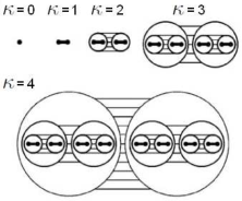
Refer to caption
Figure 5.1: Sporns’ algorithm for the fractal connectivity matrix. At the level κ=0\kappa=0 a single dot represents a group of 2μ2^{\mu} fully connected neurons. At κ=1\kappa=1 we duplicate this elementary block, obtaining two groups of 2μ2^{\mu} neurons which are linked together with a connection density E−1E^{-1}. This structure is generated again at the level κ=2\kappa=2, and connected to the previous one with a connection density E−2E^{-2}, and so on. This figure has been taken and adapted from [19].
Refer to caption
Refer to caption
Figure 5.2: Two examples of fractal matrix obtained with the Sporns’ algorithm, for η=8\eta=8, μ=4\mu=4 and E=2.0E=2.0 (left-hand side) and for η=11\eta=11, μ=2\mu=2 and E=1.5E=1.5 (right-hand side). A blue dot corresponds to a 11 in the topology matrix, while the absence of the dot corresponds to a 00. The figure on the right-hand side has been resized in order to the have the same spatial extension as the figure on the left-hand side. For this reason it does not clearly show the diagonal white line corresponding to Ji​i​(t)=0J_{ii}\left(t\right)=0, namely to the absence of self-connections.

According to [19], the parameter EE determines the path length, the clustering coefficient and the complexity of the network. The latter was first introduced in [35], and quantifies the extent to which a system is both functionally segregated and functionally integrated. This means that both the degree of independence of the blocks and their level of cooperation are taken into account by a single quantity, the complexity of the network, which for the fractal topology is maximum when E≈2E\approx 2.

Now we have to determine the quantities 𝔼⁡[Ti​j]\mathbb{E}\left[T_{ij}\right], 𝔼⁡[Ti​k​Tj​l]\mathbb{E}\left[T_{ik}T_{jl}\right], 𝔼⁡[Ti​l​Tj​m​Tk​n]\mathbb{E}\left[T_{il}T_{jm}T_{kn}\right] etc. Therefore we need to analyze the algorithm that generates the fractal connectivity matrix. If all the connections are at the level κ=0\kappa=0, where the neurons are always fully connected, then we trivially have:

𝔼⁡[Ti​j]=\displaystyle\mathbb{E}\left[T_{ij}\right]= 1−δi​j\displaystyle 1-\delta_{ij}
𝔼⁡[Ti​k​Tj​l]=\displaystyle\mathbb{E}\left[T_{ik}T_{jl}\right]= (1−δi​k)​(1−δj​l)\displaystyle\left(1-\delta_{ik}\right)\left(1-\delta_{jl}\right)
𝔼⁡[Ti​l​Tj​m​Tk​n]=\displaystyle\mathbb{E}\left[T_{il}T_{jm}T_{kn}\right]= (1−δi​l)​(1−δj​m)​(1−δk​n)\displaystyle\left(1-\delta_{il}\right)\left(1-\delta_{jm}\right)\left(1-\delta_{kn}\right)

because in this case the entries of the topology are deterministic. Moreover, if we have an entry of the topology matrix, for example Ti​kT_{ik}, at the level κ=0\kappa=0, and another entry, for example Tj​lT_{jl}, at a different level, we obtain 𝔼⁡[Ti​k​Tj​l]=(1−δi​k)​𝔼​[Tj​l]\mathbb{E}\left[T_{ik}T_{jl}\right]=\left(1-\delta_{ik}\right)\mathbb{E}\left[T_{jl}\right], and so on and so forth.

We next compute these statistical quantities when the connections are not at the level κ=0\kappa=0. At a given level κ>1\kappa>1, the total number of possible connections (in one direction) is ακ=4μ+κ−1\alpha_{\kappa}=4^{\mu+\kappa-1}, among which the algorithm has to choose randomly βκ=⌊E−κ​ακ⌋\beta_{\kappa}=\left\lfloor E^{-\kappa}\alpha_{\kappa}\right\rfloor connections.

At the level κ\kappa the probability that Ti​jT_{ij} is chosen at some time after βκ\beta_{\kappa} steps, regardless the step at which it has been actually chosen, is:

p⁡(Ti​j=1)=βκακp\left(T_{ij}=1\right)=\frac{\beta_{\kappa}}{\alpha_{\kappa}}

since we can draw uniformly among ακ\alpha_{\kappa} possible connections, therefore:

𝔼⁡[Ti​j]=0×p⁡(Ti​j=0)+1×p⁡(Ti​j=1)=βκακ\mathbb{E}\left[T_{ij}\right]=0\times p\left(T_{ij}=0\right)+1\times p\left(T_{ij}=1\right)=\frac{\beta_{\kappa}}{\alpha_{\kappa}}

Now we want to evaluate 𝔼⁡[Ti​j​Tk​l]\mathbb{E}\left[T_{ij}T_{kl}\right]. If, in the picture of the connectivity matrix, Ti​jT_{ij} and Tk​lT_{kl} are in two different squares, then clearly they are not correlated, therefore in that case we have 𝔼⁡[Ti​j​Tk​l]=𝔼⁡[Ti​j]​𝔼​[Tk​l]=βκ1ακ1​βκ2ακ2\mathbb{E}\left[T_{ij}T_{kl}\right]=\mathbb{E}\left[T_{ij}\right]\mathbb{E}\left[T_{kl}\right]=\frac{\beta_{\kappa_{1}}}{\alpha_{\kappa_{1}}}\frac{\beta_{\kappa_{2}}}{\alpha_{\kappa_{2}}}. If instead they are in the same square, we have:

𝔼⁡[Ti​j​Tk​l]=βκ​(βκ−1)ακ​(ακ−1)\mathbb{E}\left[T_{ij}T_{kl}\right]=\frac{\beta_{\kappa}\left(\beta_{\kappa}-1\right)}{\alpha_{\kappa}\left(\alpha_{\kappa}-1\right)}

since they are selected sequentially and independently from each other. In general, for nn entries of the topology in the same square, with n≤βκn\leq\beta_{\kappa}, we obtain:

𝔼⁡[Ti0​j0​Ti1​j1​…​Tin−1​jn−1]=βκ​(βκ−1)​…​(βκ−n+1)ακ​(ακ−1)​…​(ακ−n+1)=βκ!​(ακ−n)!ακ!​(βκ−n)!\mathbb{E}\left[T_{i_{0}j_{0}}T_{i_{1}j_{1}}...T_{i_{n-1}j_{n-1}}\right]=\frac{\beta_{\kappa}\left(\beta_{\kappa}-1\right)...\left(\beta_{\kappa}-n+1\right)}{\alpha_{\kappa}\left(\alpha_{\kappa}-1\right)...\left(\alpha_{\kappa}-n+1\right)}=\frac{\beta_{\kappa}!\left(\alpha_{\kappa}-n\right)!}{\alpha_{\kappa}!\left(\beta_{\kappa}-n\right)!}

thereby the problem of determining the correlation structure of the neural network with the fractal connectivity matrix is solved.

6 Numerical experiments

We want to show that this perturbative expansion provides a good match with the exact equations of the network. For this reason in Figures 6.2 and 6.3 we have shown the comparison between the membrane potential, variance, covariance and correlation of pairs of neurons for two kinds of connectivity matrices (fully connected and cycle graphs, see Figure 6.1), obtained from the simulation of equations 2.1 (blue line), of equations 2.14 - 2.18 (red line) and from formulae 3.2 - 3.8, 4.3 and 4.4 (green line). Therefore we have obtained these figures without considering the second order terms in the perturbative expansion of Vi​(t)V_{i}\left(t\right). In other words, we have omitted the third order terms 3.9 - 3.12 in the variance and covariance, due to the difficulty of implementing them numerically. Instead in Figures 6.4 and 6.5 we have shown the comparison between equations 2.1 (blue line) and equations 2.14 - 2.22 (red line), therefore considering also the higher order terms, because the numerical calculation of the variance and covariance through the simulation of equations 2.19 - 2.22 is much easier than the implementation of the terms 3.9 - 3.12.

For the networks with random topology, the analytic formulae of the variance, covariance and correlation are rather complex to implement. In fact usually the approximation of order 00 of the quantities 𝔼⁡[Ti​jMi]\mathbb{E}\left[\frac{T_{ij}}{M_{i}}\right], 𝔼⁡[Ti​k​Tj​lMi​Mj]\mathbb{E}\left[\frac{T_{ik}T_{jl}}{M_{i}M_{j}}\right] and 𝔼⁡[Ti​k​Tl​m​Tj​lMi​Mj​Ml]\mathbb{E}\left[\frac{T_{ik}T_{lm}T_{jl}}{M_{i}M_{j}M_{l}}\right] is not precise enough, forcing us to add the higher order corrections. For example, for a network with independent random connections with p⁡(Ti​j=1)=pp\left(T_{ij}=1\right)=p ∀i,j:i≠j\forall i,j:\,i\neq j, the approximation of order 00 of 𝔼⁡[Ti​jMi]\mathbb{E}\left[\frac{T_{ij}}{M_{i}}\right] is:

𝔼⁡[Ti​jMi]≈𝔼⁡[Ti​j]∑k=0N−1𝔼⁡[Ti​k]=p(N−1)​p=1N−1\mathbb{E}\left[\frac{T_{ij}}{M_{i}}\right]\approx\frac{\mathbb{E}\left[T_{ij}\right]}{{\displaystyle\sum_{k=0}^{N-1}}\mathbb{E}\left[T_{ik}\right]}=\frac{p}{\left(N-1\right)p}=\frac{1}{N-1}

which does not depend on pp and therefore does not contain information about the randomness of the topology. This means that in general this approximation is a too poor description of the random topology, and therefore the higher order corrections must be included. Unfortunately, according to 3.17, the approximations of order 11 are always equal to zero, therefore we have to extend the approximation up to the 22nd order. In other terms, we have to compute the second order derivatives in the multidimensional Taylor expansions of 𝔼⁡[Ti​jMi]\mathbb{E}\left[\frac{T_{ij}}{M_{i}}\right], 𝔼⁡[Ti​k​Tj​lMi​Mj]\mathbb{E}\left[\frac{T_{ik}T_{jl}}{M_{i}M_{j}}\right] and 𝔼⁡[Ti​k​Tl​m​Tj​lMi​Mj​Ml]\mathbb{E}\left[\frac{T_{ik}T_{lm}T_{jl}}{M_{i}M_{j}M_{l}}\right]. This is a feasible but complex task, and it is particularly hard for the fractal connectivity matrix, since it depends on the blocks the synaptic connections belong to. For this reason we have opted for showing only the comparison between the numerical simulations of the stochastic differential equations (red and blue lines), without using the analytic formulae. Figures 6.6 - 6.12 show these results for a network with independent random connections and for the Sporns’ fractal matrix. The differential equations have been solved numerically using the Euler-Maruyama scheme, while the integrals with respect to time have been calculated using the trapezoidal rule, in both cases with an integration time step Δ​t=0.1\Delta t=0.1. All the statistics have been evaluated with 10,00010,000 Monte Carlo simulations (where we have independently generated repetitions of the four sources of randomness of the system), while the remaining parameters are reported in Table 6.1. The covariance and correlation have always been calculated between the 00th and the 11st neuron. The only exceptions are in Figures 6.10, 6.11 and 6.12, where the comparison is between the 00th and the 88th neuron. Instead the membrane potentials and the variances have always been reported only for the the 00th neuron. In general we have obtained a better agreement with the exact equations when we use also the second order corrections of the membrane potential.

It is important to observe that a detailed analysis of the error introduced by the perturbative expansion as a function of the approximation order, the values of all the parameters of the system and the infinitely many connectivity matrices is missing and is beyond the purpose of this article.

Neuron Input
τ=1\tau=1 Ii​(t)={s​i​n​(2​t),i=0÷N2−10.2+e−t,i=N2÷N−1I_{i}\left(t\right)=\begin{cases}sin\left(2t\right),&\begin{array}[]{c}i=0\div\frac{N}{2}-1\end{array}\\ 0.2+e^{-t},&\begin{array}[]{c}i=\frac{N}{2}\div N-1\end{array}\end{cases}
C2=0.5C_{2}=0.5 C1=0.4C_{1}=0.4
σ2=0.1\sigma_{2}=0.1 σ1=0.01\sigma_{1}=0.01
μi={−1,i=0÷N2−10.5,i=N2÷N−1\mu_{i}=\begin{cases}-1,&\begin{array}[]{c}i=0\div\frac{N}{2}-1\end{array}\\ 0.5,&\begin{array}[]{c}i=\frac{N}{2}\div N-1\end{array}\end{cases}
Synaptic Weights Sigmoid Function
J¯^i​j​(t)={(1+t2)−1,i,j=0÷N2−1cos⁡(t),i=0÷N2−1,j=N2÷N−11+2π​arctan⁡(t),i=N2÷N−1,j=0÷N2−1e−t​sin⁡(t),i,j=N2÷N−1\widehat{\overline{J}}_{ij}\left(t\right)=\begin{cases}\left(1+t^{2}\right)^{-1},&\begin{array}[]{c}i,j=0\div\frac{N}{2}-1\end{array}\\ \cos\left(t\right),&\begin{array}[]{ccc}i=0\div\frac{N}{2}-1,&&j=\frac{N}{2}\div N-1\end{array}\\ \sqrt{1+\frac{2}{\pi}\arctan\left(t\right)},&\begin{array}[]{ccc}i=\frac{N}{2}\div N-1,&&j=0\div\frac{N}{2}-1\end{array}\\ e^{-t}\sin\left(t\right),&\begin{array}[]{c}i,j=\frac{N}{2}\div N-1\end{array}\end{cases} TM​A​X=1T_{MAX}=1
C3=0.6C_{3}=0.6 λ=1\lambda=1
σ3=0.1\sigma_{3}=0.1 VT=0V_{T}=0
Table 6.1: Parameters used to generate Figures 6.2 - 6.12
Refer to caption
Refer to caption
Figure 6.1: Network topologies used to generate Figures 4.1 and 6.2 - 6.5. In the context of Graph Theory, KNK_{N} is called complete graph and represents the topology of a fully connected network, while C​yNCy_{N} is called cycle graph and represents the case when the neurons are connected to form a closed loop.
Refer to caption
Refer to caption
Refer to caption
Refer to caption
Figure 6.2: Comparison of the variance, covariance and correlation obtained from the simulation of equations 2.1 (blue line), of equations 2.14 - 2.18 (red line) and from formulae 3.2 - 3.8, 4.3 and 4.4 (green line). Therefore the perturbative expansion of the membrane potential has been truncated at the first order, while those of the variance and covariance at the second order. We have compared the 00th and the 11st neuron, using the Euler-Maruyama scheme (blue and red lines) and the trapezoidal rule (green line) with integration time step Δ​t=0.1\Delta t=0.1. The statistics have been evaluated with 10,00010,000 Monte Carlo simulations, for the values of the parameters reported in Table 6.1. The topology is K10K_{10} (see Figure 6.1) and therefore deterministic.
Refer to caption
Refer to caption
Refer to caption
Refer to caption
Figure 6.3: Comparison of the variance, covariance and correlation obtained for the deterministic topology C​y10Cy_{10} (see Figure 6.1), for the values of the parameters reported in Table 6.1.
Refer to caption
Refer to caption
Refer to caption
Figure 6.4: Comparison of the variance, covariance and correlation obtained for the deterministic topology K10K_{10}, for the values of the parameters reported in Table 6.1, but considering also the second order corrections of the membrane potential. Clearly the match has been improved by the addition of these terms, as the reader can easily check from the comparison with Figure 6.2.
Refer to caption
Refer to caption
Refer to caption
Figure 6.5: Comparison of the variance, covariance and correlation obtained for the deterministic topology C​y10Cy_{10}, for the values of the parameters reported in Table 6.1, but considering also the second order corrections of the membrane potential. This time the improvement of the match is not evident, if compared with Figure 6.3, which proves that the goodness of the perturbative expansion depends also on the topology of the network. It is important to observe that the second order corrections are generally small, therefore their magnitude could be of the same order of the numerical error introduced by the finite number of Monte Carlo simulations.
Refer to caption
Refer to caption
Refer to caption
Figure 6.6: Comparison of the variance, covariance and correlation obtained for a random topology, for the values of the parameters reported in Table 6.1, considering also the second order corrections of the membrane potential. In detail, here we have assumed that each pair of neurons is connected independently from the others and with probability p=0.7p=0.7. Even if the match of the variance and covariance is quantitatively very good, the approximation of the correlation is not satisfying for t>2t>2. This is due to the fact that the ratio of small quantities (in this case the variance and covariance) is very sensitive to small errors in the numerator and denominator. Nevertheless the second order expansion provides a satisfying result, because the variance and covariance are in very good agreement with the exact neural equations. It is important to observe that the discrepancy is also due to the finite number of Monte Carlo simulations, which should be increased especially for small values of the variance and covariance.
Refer to caption
Refer to caption
Refer to caption
Figure 6.7: Comparison of the variance, covariance and correlation obtained for the Sporns’ topology, for the values of the parameters reported in Table 6.1, considering also the second order corrections of the membrane potential. In this example we have set η=4\eta=4 (N=16N=16), μ=2\mu=2 and E=1.1E=1.1, therefore the network is almost fully connected. The two neurons are in the same block, therefore they are connected at the level κ=0\kappa=0.
Refer to caption
Refer to caption
Refer to caption
Figure 6.8: As in the Figure 6.7, but with E=2E=2. This, according to [19], is approximately the point of maximum complexity of the network, see text.
Refer to caption
Refer to caption
Refer to caption
Figure 6.9: As in the Figure 6.7, but with E=5E=5. In this case the blocks are almost completely disconnected. From the comparison with Figures 6.7 and 6.8, the reader can easily check that the increase of the parameter EE determines the reduction of the correlation at large tt, as a consequence of the diminution of the number of connections.
Refer to caption
Refer to caption
Refer to caption
Figure 6.10: Comparison of the variance, covariance and correlation obtained for the Sporns’ topology, for the values of the parameters reported in Table 6.1, considering also the second order corrections of the membrane potential. In this example we have set η=4\eta=4 (N=16N=16), μ=2\mu=2 and E=1.1E=1.1, as in Figure 6.7, but now the neurons are in two different blocks, and they are connected at the level κ=2\kappa=2.
Refer to caption
Refer to caption
Refer to caption
Figure 6.11: As in the Figure 6.10, but with E=2E=2.
Refer to caption
Refer to caption
Refer to caption
Figure 6.12: As in the Figure 6.10, but with E=5E=5. Again, the increase of the parameter EE determines the reduction of the correlation for large tt. It is important to observe that the difference between the two cases with the neurons in the same block or in two different blocks is very small. This is due to the fact that the values of the parameters C1C_{1}, C2C_{2} and C3C_{3} are relatively high (see Table 6.1), therefore they strongly determine the behavior of the correlation, for every topology. When these parameters are set to zero, a richer behavior of the correlation emerges. This analysis is not shown in the article, because the purpose of this work is to develop mathematical tools that allow us to understand a neural network, not the analysis of the consequences of the formulae.

7 Conclusion

We have shown how to study the correlation structure of a stochastic neural network with a finite size and a generic connecivity matrix.

This analysis has been performed using a second order perturbative analysis in terms of the standard deviations of the sources of randomness in the system and also in terms of the strength of the synaptic weights.

All the distributions are supposed to be normal, which has allowed us to obtain analytic results using the Isserlis’ theorem.

This calculation has been developed for both deterministic and random topologies of the synaptic connections, and applied to a biologically relevant case with fractal nested structure.

Moreover the numerical comparison with the exact neural equations has shown a good agreement if the perturbative parameters are small enough.

Therefore this technique can be used to study neurons with complicated connections and to reveal the relation between the covariance matrix of the membrane potentials, namely the functional connectivity of the system, and the matrix J⁡(t)J\left(t\right), also known as structural or anatomical connectivity.

The perturbative analysis developed in this article can also be extended easily to study the correlation structure of rate neurons with synaptic plasticity or learning, namely when the intensities of the synaptic weights are not chosen a priori, but are generated by other differential equations.

This idea can also be extended to spiking neurons, like those described by the FitzHugh-Nagumo [36][37], Morris-Lecar [38] or Hodgkin-Huxley [39] equations.

The only problem with these models is that they are not analytically solvable even when the neurons are disconnected, because the differential equation of Y0i​(t)Y_{0}^{i}\left(t\right) becomes non-linear.

Nevertheless the equations satisfied by the other functions Ymi​(t)Y_{m}^{i}\left(t\right) and Ym,ni​(t)Y_{m,n}^{i}\left(t\right) are linear, therefore in this case we can determine the correlation structure of the system semi-analytically.

In other words, all the results will be expressed in terms of analytic functions of Y0i​(t)Y_{0}^{i}\left(t\right), which is not analytically known, but must be solved numerically.

To conclude, we remind that the results of this article can be applied only to the case of weak synaptic weights and when the slope of the activation function is not too large, so the next step will be the development of a theory which describes the behavior of the network under more general hypotheses.

Acknowledgements

This work was partially supported by the ERC grant #227747 NerVi, the FACETS-ITN Marie-Curie Initial Training Network #237955 and the IP project BrainScaleS #269921.

References

  • [1] J. G. White, E. Southgate, J. N. Thomson, and S. Brenner. The Structure of the Nervous System of the Nematode Caenorhabditis Elegans. Philosophical Transactions of the Royal Society. B, Biological Sciences, 314(1165):1–340, 1986.
  • [2] L. R. Varshney, B. L. Chen, E. Paniagua, D. H. Hall, and D. B. Chklovskii. Structural Properties of the Caenorhabditis Elegans Neuronal Network. PLoS Computational Biology, 7(2):e1001066, February 2011.
  • [3] Mouse Connectome Project. www.mouseconnectome.org.
  • [4] K. L. Briggman, M. Helmstaedter, and W. Denk. Wiring Specificity in the Direction-Selectivity Circuit of the Retina. Nature, 471(7337):183–188, March 2011.
  • [5] D. D. Bock, W.-C. A. Lee, A. M. Kerlin, M. L. Andermann, G. Hood, A. W. Wetzel, S. Yurgenson, E. R. Soucy, H. S. Kim, and R. C. Reid. Network Anatomy and In Vivo Physiology of Visual Cortical Neurons. Nature, 471(7337):177–182, March 2011.
  • [6] G. A. P. C. Burns and M. P. Young. Analysis of the Connectional Organization of Neural Systems Associated with the Hippocampus in Rats. Philosophical Transactions of the Royal Society. B, Biological Sciences, 355(1393):55–70, 2000.
  • [7] O. Schmitt, P. Eipert, K. Philipp, R. Kettlitz, G. Fuellen, and A. Wree. The Intrinsic Connectome of the Rat Amygdala. Front Neural Circuits, 6:81, 2012.
  • [8] J. W. Scannell, C. Blakemore, and M. P. Young. Analysis of Connectivity in the Cat Cerebral Cortex. Journal of Neuroscience, 15:1463, 1995.
  • [9] J. W. Scannell, G. A. P. C. Burns, C. C. Hilgetag, M. A. O’Neil, and M. P. Young. The Connectional Organization of the Cortico-Thalamic System of the Cat. Cerebral Cortex, 9(3):277–299, April 1999.
  • [10] Daniel J. F. and David C. V. E. Distributed Hierarchical Processing in the Primate Cerebral Cortex. Cerebral Cortex, pages 1–47, 1991.
  • [11] O. Sporns, G. Tononi, and R. Kötter. The Human Connectome: A Structural Description of the Human Brain. PLoS Computational Biology, 1(4):e42, September 2005.
  • [12] O. Sporns. The Human Connectome: A Complex Network. Annals of the New York Academy of Sciences, 1224(1):109–125, 2011.
  • [13] Human Connectome Project. www.humanconnectomeproject.org.
  • [14] D. J. Watts and S. H. Strogatz. Collective Dynamics of ’Small-World’ Networks. Nature, 393(6684):409–10, 1998.
  • [15] D. S. Bassett and E. Bullmore. Small-World Brain Networks. The Neuroscientist, 12(6):512–523, 2006.
  • [16] C. J. Stam and J. C. Reijneveld. Graph Theoretical Analysis of Complex Networks in the Brain. Nonlinear Biomedical Physics, 1(1):3, 2007.
  • [17] V. B. Mountcastle. Modality and Topographic Properties of Single Neurons of Cat’s Somatic Sensory Cortex. Journal of Neurophysiology, 20:408–434, 1957.
  • [18] F. Grimbert. Mesoscopic Models of Cortical Structures. PhD thesis, 2007.
  • [19] O. Sporns. Small-World Connectivity, Motif Composition, and Complexity of Fractal Neuronal Connections. Biosystems, 85(1):55–64, July 2006.
  • [20] S. C. Ponten, A. Daffertshofer, A. Hillebrand, and C. J. Stam. The Relationship Between Structural and Functional Connectivity: Graph Theoretical Analysis of an EEG Neural Mass Model. NeuroImage, 52(3):985–994, 2010.
  • [21] V. Pernice, B. Staude, S. Cardanobile, and S. Rotter. How Structure Determines Correlations in Neuronal Networks. PLoS Computational Biology, 7(5):e1002059, May 2011.
  • [22] O. Sporns, D. Chialvo, M. Kaiser, and C. Hilgetag. Organization, Development and Function of Complex Brain Networks. Trends in Cognitive Sciences, 8(9):418–425, September 2004.
  • [23] C. J. Honey, O. Sporns, L. Cammoun, X. Gigandet, J. P. Thiran, R. Meuli, and P. Hagmann. Predicting Human Resting-State Functional Connectivity From Structural Connectivity. Proceedings of the National Academy of Sciences, 106(6):2035–2040, 2009.
  • [24] H. E. Pol, M. P. van den Heuvel, R. C. W. Mandl, R. S. Kahn, and H. E. Hulshoff Pol. Functionally Linked Resting-State Networks Reflect the Underlying Structural Connectivity Architecture of the Human Brain. Human Brain Mapping, 30:3127–3141, 2009.
  • [25] E. Rykhlevskaia, G. Gratton, and M. Fabiani. Combining Structural and Functional Neuroimaging Data for Studying Brain Connectivity: A Review. Psychophysiology, 45(2):173–187, March 2008.
  • [26] J. Touboul, G. Hermann, and O. Faugeras. Noise-Induced Behaviors in Neural Mean Field Dynamics. SIAM Journal on Applied Dynamical Systems, 11(1):49–81, 2012.
  • [27] J. Baladron, D. Fasoli, O. Faugeras, and J. Touboul. Mean-Field Description and Propagation of Chaos in Networks of Hodgkin-Huxley and FitzHugh-Nagumo neurons. The Journal of Mathematical Neuroscience, 2(1):10, May 2012. This work was partially supported by the ERC grant #227747 NerVi, the FACETSITN Marie-Curie Initial Training Network #237955 and the IP project BrainScaleS #269921.
  • [28] D. Fasoli and O. Faugeras. Finite Size Effects in the Correlation Structure of Stochastic Neural Networks: Analysis of Different Connectivity Matrices and Failure of the Mean-Field Theory. arxiv.org/abs/1307.2129, 2013. This work was partially supported by the ERC grant #227747 NerVi, the FACETSITN Marie-Curie Initial Training Network #237955 and the IP project BrainScaleS #269921.
  • [29] S.-I. Amari. Characteristics of Random Nets of Analog Neuron-Like Elements. IEEE Transactions on Systems, Man, and Cybernetics, 2(5):643–657, 1972.
  • [30] S.-I. Amari. Dynamics of Pattern Formation in Lateral-Inhibition Type Neural Fields. Biological Cybernetics, 27:77–87, 1977.
  • [31] H. R. Wilson and J. D. Cowan. Excitatory and Inhibitory Interactions in Localized Populations of Model Neurons. Biophysics, pages 1–24, 1972.
  • [32] H. R. Wilson and J. D. Cowan. A Mathematical Theory of the Functional Dynamics of Cortical and Thalamic Nervous Tissue. Kybernetik, 13:55–80, 1973.
  • [33] L. Isserlis. On a Formula for the Product-Moment Coefficient of any Order of a Normal Frequency Distribution in any Number of Variables. Biometrika, 12(1/2):134–139, 1918.
  • [34] C. Viroli. Finite Mixtures of Matrix Normal Distributions for Classifying Three-Way Data. Statistics and Computing, 21(4):511–522, 2011.
  • [35] G. Tononi, G. M. Edelman, and O. Sporns. Complexity and Coherency: Integrating Information in the Brain. Trends in Cognitive Sciences, 2(12):474–484, December 1998.
  • [36] R. FitzHugh. Impulses and Physiological States in Theoretical Models of Nerve Membrane. Biophysical Journal, 1(6):445–466, July 1961.
  • [37] J. Nagumo, S. Arimoto, and S. Yoshizawa. An Active Pulse Transmission Line Simulating Nerve Axon. Proceedings of the Institute of Radio Engineers, 50(10):2061–2070, 1962.
  • [38] C. Morris and H. Lecar. Voltage Oscillations in the Barnacle Giant Muscle Fiber. Biophysical Journal, 35:193–213, 1981.
  • [39] A. L. Hodgkin and A. F. Huxley. A Quantitative Description of Membrane Current and its Application to Conduction and Excitation in Nerve. The Journal of Physiology, 117(4):500–544, August 1952.