Convergence of an Iterative Algorithm for Teichmüller Maps via Generalized Harmonic Maps
Abstract
Finding surface mappings with least distortion arises from many applications in various fields. Extremal Teichmüller maps are surface mappings with least conformality distortion. The existence and uniqueness of the extremal Teichmüller map between Riemann surfaces of finite type are theoretically guaranteed [1]. Recently, a simple iterative algorithm for computing the Teichmüller maps between connected Riemann surfaces with given boundary value was proposed in [11]. Numerical results was reported in the paper to show the effectiveness of the algorithm. The method was successfully applied to landmark-matching registration. The purpose of this paper is to prove the iterative algorithm proposed in [11] indeed converges.
keywords
Teichmüller map, extremal map, quasiconformal map, harmonic energy optimization, registration.1 Introduction
Finding meaningful surface mappings with least distortion has fundamental importance. Applications can be found in different areas such as registration, shape analysis and grid generation. Conformal mapping has been widely used to establish a good one-to-one correspondence between different surfaces, since it preserves the local geometry well [2, 3, 4, 5, 6, 7, 8, 9, 10]. The Riemann mapping theorem guarantees the existence of conformal mappings between simply-connected surfaces. However, this fact is not valid for general Riemann surfaces. Given two Riemann surfaces with different conformal modules, there is generally no conformal mapping between them. In this case, it is usually desirable to obtain a mapping that minimizes the conformality distortion. Every diffeomorphic surface mapping is associated with a unique Beltrami differential, which is a complex-valued function, , defined on the source surface. The Beltrami differential, , measures the deviation of the mapping from a conformal map. Given two Riemann surfaces and , there exists a unique and bijective map , called the Teichmüller map, minimizing the norm of the Beltrami differential [1]. Therefore, the extremal Teichmüller map can be considered as the ‘most conformal’ map between Riemann surfaces of the same topology, which is a natural extension of conformal mappings.
1.1 Extremal problem
Mathematically, the extremal problem for obtaining a surface mapping with least conformality distortion can be formulated as follows. Suppose and are two Riemann surfaces of finite type, where and are their conformal parameters respectively. Every diffeomorphism between and is associated with a unique Beltrami differential. A Beltrami differential on the Riemann surface is an assignment to each chart of an complex-valued function , defined on local parameter . Then, is said to be a quasi-conformal mapping associated with the Beltrami differential if for any chart on and any chart on , the mapping is quasi-conformal associated with .
Our goal is to look for an extremal quasi-conformal mapping, which are extremal in the sense of minimizing the over all Beltrami differentials corresponding to quasi-conformal mappings between and . The idea of extremality is to make the supreme norm of the Beltrami differential as small as possible such that is as ‘nearly conformal’ as possible.
The extremal problem can therefore be formulated as finding that solves:
| (1) |
where .
The above optimization problem (1) has a unique global minimizer provided that and are Riemann surfaces of finite type. Also, the unique minimizer is a Teichmüller map, that is, its associated Beltrami differential is of the following form:
| (2) |
where is a non-negative real constant and is an integrable holomorphic function defined on (). Beltrami differential of this form is said to be of Teichmüller type.
1.2 An iterative algorithm for Teichmüller maps
To solve the extremal problem (1) to obtain the Teichmüller map between connected surfaces, an iterative algorithm was proposed in [11], called the quasi-conformal(QC) iteration. The ultimate goal is to obtain the extremal map between connected (either simply-connected or multiply-connected) surfaces with given boundary value, which minimizes the conformality distortion. The basic idea of the iterative algorithm is to project the Beltrami differential to the space of all Beltrami differentials of Teichmüller type, and compute a quasi-conformal map whose Beltrami differential is closest to the projection in the least square sense. More specifically, the QC iteration for solving (1) can be described as follows.
| (3) |
where is the quasi-conformal map obtained at the iteration, is the Beltrami differential of and is a Beltrami differential of constant modulus.
is the operator to obtain a quasi-conformal mapping whose Beltrami differential is closest to in the least square sense. In other words,
| (4) |
denotes the Beltrami differential of under the auxiliary metric with respect to , namely, ( is the original metric on ). More precisely, can be explicitly computed as follows:
| (5) |
is the operator to project to the space of Beltrami differentials with constant modulus. It is defined as:
| (6) |
where and is a suitable real function on such that is a constant.
In practice, the projection operator can be simplified as
| (7) |
is the Laplacian smoothing operator to smooth out .
Both , and can be easily computed. In particular, the discretization of on a triangulation mesh can be reduced to a least square problem of a linear system.
When is small, can be chosen to be 1. Then, , where is the Beltrami differential of under the original metric.. The QC iteration can be further modified as
| (8) |
The QC iteration (3) is very efficient. Also, numerical results reported in [11] demonstrate that the proposed iteration can compute the Teichmüller map accurately, even on highly irregular meshes. The algorithm was successfully applied to landmark-based registration for applications in medical imaging and computer graphics.
This paper is to provide a complete analysis of the above iterative algorithm (3). In particular, we prove the convergence of (3) that and respectively converges to the extremal map and its associated Beltrami differential , which solves the optimization problem (1).
We remark that although the iterative algorithm is designed for obtaining extremal map between connected surfaces with given boundary values, the convergence proof applies to general Riemann surfaces of finite type (such as high-genus closed surfaces). In other words, the QC iteration can be applied to computing extremal maps between general Riemann surfaces. For the ease of the presentation, we will restrict our discussion to the situation when both and are either simply-connected or multiply-connected open surfaces.
1.3 Organization
This paper is organized as follows. In Section 2, we describe some mathematical background, which is relevant to this work. In Section 3, we reformulate the extremal problem defined by (1) as the optimization problem of the harmonic energy, which helps us to understand the iterative algorithm (3) better. In Section 4, we prove the convergence of the QC iteration to our desired extremal Teichmüller map. A concluding remark will be given in Section 6.
2 Mathematical background
2.1 Quasi-conformal mappings and Beltrami equation
In this section, we describe some basic mathematical concepts relevant to our algorithms. For details, we refer the readers to [12, 13].
A surface with a conformal structure is called a Riemann surface. Given two Riemann surfaces and , a map is conformal if it preserves the surface metric up to a multiplicative factor called the conformal factor. A generalization of conformal maps is the quasi-conformal maps, which are orientation preserving homeomorphisms between Riemann surfaces with bounded conformality distortion, in the sense that their first order approximations takes small circles to small ellipses of bounded eccentricity [12]. Mathematically, is quasi-conformal provided that it satisfies the Beltrami equation:
| (9) |
for some complex-valued function satisfying . is called the Beltrami coefficient, which is a measure of non-conformality. measures how far the map is deviated from a conformal map. if and only if is conformal. Infinitesimally, around a point , may be expressed with respect to its local parameter as follows:
| (10) |

Obviously, is not conformal if and only if . Inside the local parameter domain, may be considered as a map composed of a translation to together with a stretch map , which is postcomposed by a multiplication of . All the conformal distortion of is caused by . is the map that causes to map a small circle to a small ellipse. From , we can determine the directions of maximal magnification and shrinking and the amount of their distortions as well. Specifically, the angle of maximal magnification is with magnifying factor ; The angle of maximal shrinking is the orthogonal angle with shrinking factor . Thus, the Beltrami coefficient gives us all the information about the properties of the map (see Figure 1).
The maximal dilation of is given by:
| (11) |
Quasiconformal mapping between two Riemann surfaces and can also be defined. Instead of the Beltrami coefficient, the Beltrami differential has to be used. A Beltrami differential on the Riemann surface is an assignment to each chart of an complex-valued function , defined on local parameter such that
| (12) |
on the domain which is also covered by another chart , where and .

An orientation preserving diffeomorphism is called quasi-conformal associated with if for any chart on and any chart on , the mapping is quasi-conformal associated with . See Figure 2 for an illustration.
2.2 Extremal maps and Teichmüller maps
A special class of quasi-conformal maps is called the extremal maps, which minimize the conformality distortion. More specifically, an extremal quasi-conformal map between and is extremal in the sense of minimizing the over all Beltrami differentials corresponding to quasi-conformal mappings between the two surfaces. Extremal map always exists but need not to be unique. Mathematically, an extremal quasi-conformal mapping can be defined as follows:
2.1.
Suppose and are connected Riemann surfaces with boundaries. Let be a quasi-conformal mapping between and . is said to be an extremal map if for any quasi-conformal mapping isotopic to relative to the boundary,
| (13) |
It is uniquely extremal if the inequality (13) is strict.
Closely related to the extremal map is the Teichmüller map. It is defined as follows.
2.2.
Let be a quasi-conformal mapping. is said to be a Teichmüller map associated to the integrable holomorphic function if its associated Beltrami differential is of the form:
| (14) |
for some constant and holomorphic function with .
In other words, a Teichmüller map is a quasi-conformal mapping with uniform conformality distortion over the whole domain.
Extremal map might not be unique. However, a Teichmüller map associated with a holomorphic function is the unique extremal map in its homotopic class. In particular, a Teichmuller map between two connected open surfaces with suitable given boundary values is the unique extremal map. The Strebel’s theorem explains the relationship bewtween the Teichmüller map and extremal map.
2.3 (Boundary dilation).
The boundary dilation of is defined as:
| (15) |
where is the family of quasi-conformal homeomorphisms of onto which are homotopic to modulo the boundary.
2.4 (Strebel’s theorem, See [14], page 319).
Let be an extremal quasi-conformal map with . If , then is a Teichmüller map associated with an integrable holomorphic function on . Hence, is also an unique extremal mapping.
In other words, an extremal map between and with suitable boundary condition is a Teichmüller map. In particular, the Teichmüller mapping and extremal mapping of the unit disk are closely related.
2.5 (See [15], page 110).
Let be an orientation-preserving homeomorphism of . Suppose further that and is bounded. Then there is a Teichmüller map that is the unique extremal extension of to . That is, is an extremal mapping with .
Thus, if the boundary correspondence satisfies certain conditions on its derivatives, the extremal map of the unit disk must be a Teichmüller map.
Now, in the case when interior landmark constraints are further enforced, the existence of unique Teichmüller map can be guaranteed if the boundary and landmark correspondence satisfy suitable conditions. The unique Teichmüller map is extremal, which minimizes the maximal conformality distortion. The following theorem can be derived immediately from the Strebel’s Theorem (Theorem 2.4):
2.6.
Let and be the corresponding interior landmark constraints. Let be the extremal map, such that corresponds to for all . If , then is a Teichmüller map associated with an integrable holomorphic function on . Hence, is an unique extremal map.
In particular, a unique Teichmüller map between unit disks with interior landmark constraints enforced exists, if the boundary map satisfies suitable conditions. The following theorem can be obtained directly from Theorem 2.5:
2.7.
Let be an orientation-preserving homeomorphism of . Suppose further that and is bounded. Let and be the corresponding interior landmark constraints. Then there is a Teichmüller map matching the interior landmarks, which is the unique extremal extension of to . That is, is an extremal Teichmüller map with matching the interior landmarks.
2.3 Harmonic maps
Our iterative algorithm to compute Teichmüller maps is closely related to harmonic maps. Let and be two Riemann surfaces of finite type, where and refer to the local conformal coordinate on the surface and .
For a Lipschitz map , we define the energy of the map to be
| (16) |
Therefore
| (17) |
It depends on the metric structure of the target surface and the conformal structure of the source.
A critical point of this functional is called a harmonic map. We will focus on the situation where we have fixed the homotopy class of maps into the compact target with non-positive curvature everywhere. In that case, there is a unique harmonic map in the homotopy class of . If is harmonic, then
| (18) |
The pull back metric on induced by is given by
| (19) |
Then the Hopf differential is
| (20) |
It can be shown that is harmonic if and only if its Hopf differential is a holomorphic quadratic differential.
3 Quasi-conformal iteration
Before giving a complete analysis of the convergence of the QC iteration, we reformulate the extremal problem (1) as the optimization problem of the harmonic energy, in order to better understand the iterative algorithm.
Consider two connected open surfaces and with boundaries, which are of the same topology. and can either be simply-connected or multiply-connected. Suppose and are the Riemannian metric on and respectively. Assume ) has non-positive Gaussian curvature everywhere. Let be any quasi-conformal mapping between and . In the homotopic class of , there exists a unique Teichmüller map, . is also extremal within the homotopic class . More specifically, the homotopic class can be defined as:
| (21) |
We have, for all , where and are the Beltrami differentials of and respectively.
Consider the space of all admissible Beltrami differentials on , which is denoted by . Every Beltrami differential induces a conformal structure on , namely,
| (22) |
Suppose , we say that they are globally equivalent, if there is a biholomorphic mapping such that is homotopic to the identity map of . The equivalence class of is represented by . Each global equivalence class of Beltrami differentials has a unique representative of Teichmüller form. We denote the space of all Beltrami differentials of Teichmüller form by
| (23) |
We can now define an energy functional on . For any , there exists a unique harmonic map , which is solely determined by and . The value of can then be defined as the harmonic energy of . That is,
| (24) |
is a smooth function.
Lemma 1.
The energy functional is bounded below by
| (25) |
where . The equality holds if and only if is conformally equivalent to . And the harmonic map is a conformal mapping.
Proof.
Let be the local coordinate of . The Jacobian of the mapping is given by
| (26) |
Therefore,
| (27) |
The harmonic energy is given by
| (28) |
where
| (29) |
| (30) |
Hence,
| (31) |
Equality holds if and only if , namely, . This implies is a conformal mapping. ∎
Theorem 2.
The global minimizer of the energy functional is the Beltrami differerntial associated to the unique Teichmüller map between and in the homotopic class of .
Proof.
Let be the Beltrami differential of the Teichmüller map . It suffices to show that is a conformal mapping.
To see this, let denote the pull back metric. Then,
| (32) |
Under the pull back metric, the mapping is isometric. We have
| (33) |
Hence,
| (34) |
So, . is conformal to . We conclude that is conformal. According to Theorem 1, the Beltrami differential associated to is the global minimizer of . ∎
In other words, finding the extremal Teichmüller map, , is equivalent to minimizing the energy functional . During the QC iteration, the Beltrami differential is iteratively adjusted and a new map is obtained by . It turns out is equivalent to computing the harmonic map . It can be explained in more details as follows.
Lemma 3.
Suppose . The mapping is a harmonic map between and .
Proof.
Let be the coordinates of with respect to the metric . Let be the harmonic map between and . Then is a critical point of the following harmonic energy:
Since , according to the definition, is the critical point of the following energy functional:
We will show that the above two energy functionals have the same set of critical points.
Note that , then
| (35) |
We obtain
| (36) |
Hence,
| (37) |
Now, the Jacobian of and the Jacobian of are given by
| (38) |
Hence,
| (39) |
Since , is a constant. Thus,
| (40) |
where is the surface area of . We conclude that and has the same set of critical points. Since is a critical point of , is also a critical point of . Hence, is a harmonic map between and . ∎
The Beltrami differential is iteratively adjusted during the QC iteration. In the next section, we will prove that monotonically decreases to the global minimizer of .
4 Proof of convergence
In this section, we prove the convergence of the Quasi-conformal iteration to the desired Teichmüller map.
Lemma 4.
Suppose is deformed by
Then, the variation of satisfies:
where is the coordinates of under the metric .
Proof.
Let be the coordinate of under the metric . For simplicity, let . Then, we have
| (41) |
The area element with respect to is given by
| (42) |
Hence,
| (43) |
Similarly,
| (44) |
Let . Then,
| (45) |
Therefore,
| (46) |
Similarly,
| (47) |
As a result, we get
| (48) |
This completes the proof of the inequality. ∎
Theorem 5.
Suppose . For any , there exists and such that:
(i) ;
(ii) and for all ;
(iii) .
Proof.
Let and . Pick such that:
| (49) |
Consider .
Suppose:
| (50) |
Let:
| (51) |
If , choose .
If , choose .
If (including ), choose .
Let:
| (52) |
By definition, . Hence, (i) is satisfied.
Now,
| (53) |
Also,
| (54) |
Thus, (ii) is also satisfied.
Finally, it is easy to check that:
| (55) |
Now, if ,
| (56) |
If ,
| (57) |
We conclude that and hence (iii) is satisfied. ∎
We can now proceed to prove the convergence of the Quasi-conformal iteration.
Theorem 6.
Suppose and are open Riemann surfaces with boundaries of the same topology. Given a smooth boundary correspondence , the Quasi-conformal (QC) iteration (3) converges to the unique extremal map, which is also a Teichmüller map.
Proof.
Suppose the pair is obtained at the iteration. The QC iteration first compute a new quasi-conformal map by . According to Lemma 3, is a harmonic map between and . The Beltrami differential of can be computed by . denotes the Beltrami differential of under the auxiliary metric with respect to , namely, . A new Beltrami differential can then be obtained by projecting onto to get
| (58) |
Here, and is a suitable real function on such that , where is a positive constant.
According to Theorem 5, by choosing a suitable , we can assume that
| (59) |
is then smoothed out by the Laplacian operator with the constraint that it still preserves Equation 59. We get that
| (60) |
Hence, is monotonically decreasing. According to Lemma 1, is bounded from below. Hence, converges. Also, the QC iteration is essential the gradient descend algorithm of and it converges at the critical point . That is, . In this case, is conformal to and hence is a quasi-conformal map with Beltrami differential . Furthermore, at the critical point, the Laplacian of the Beltrami differential is zero. We conclude that is harmonic. Since is harmonic, we can find its harmonic conjugate such that is holomorphic. Define , which is also holomorphic. Then, is of Teichmüller type. Since is of Teichmüller type, must be a Teichmüller map. Now, given a smooth boundary correspondence , there exists a unique Teichmüller map which is an extremal map. We conclude that is the unique extremal Teichmüller map. ∎
5 Numerical experiments
Although the numerical testing is not the main focus of this work, we demonstrate some numerical results in this section for the completeness of the paper. The results agree with our theoretical findings.
Example 1
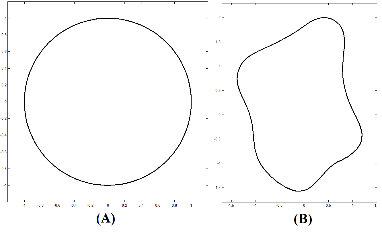
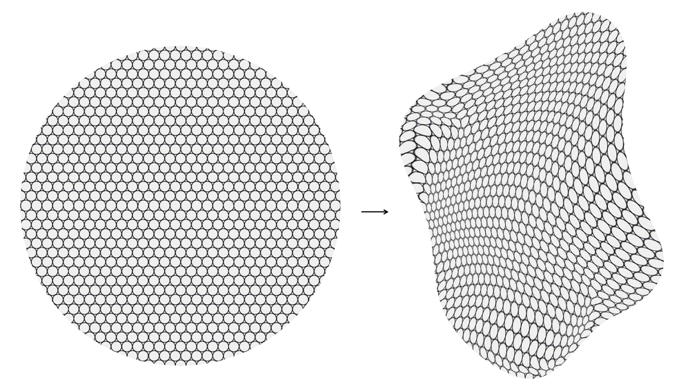
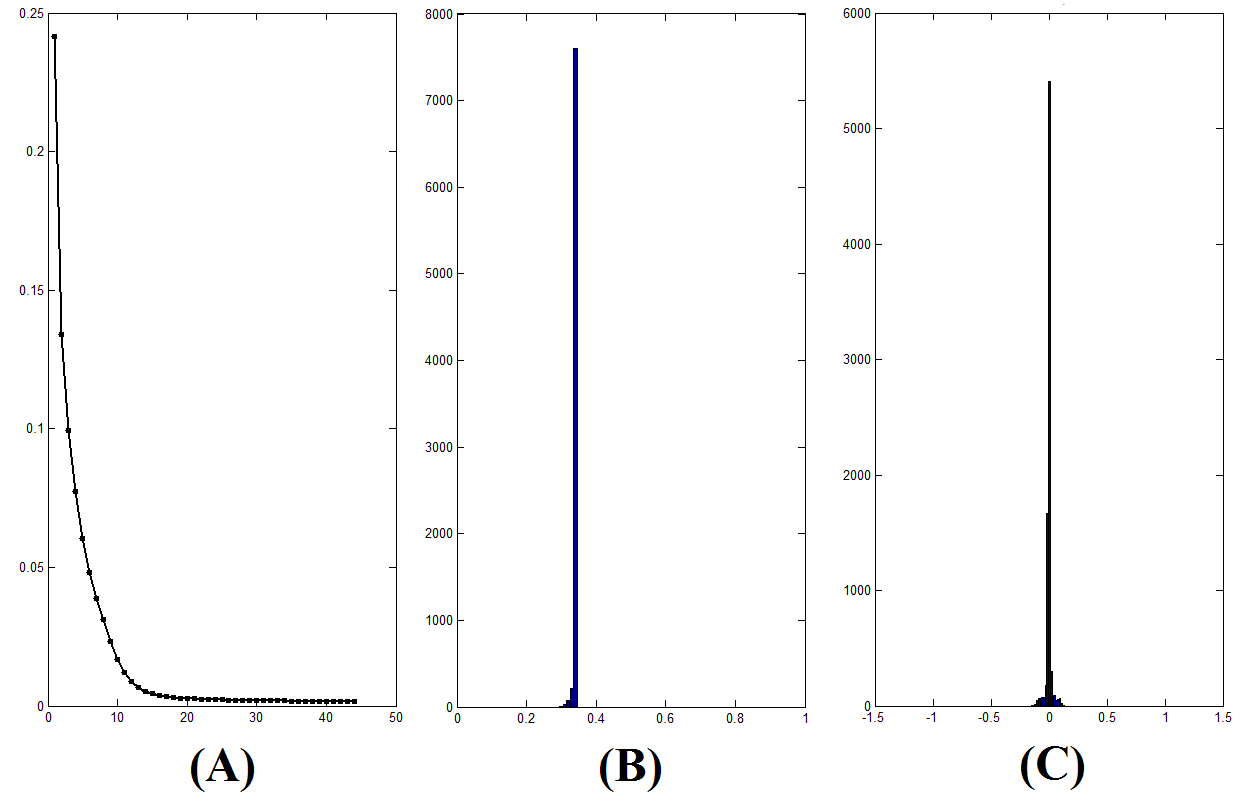
We first test the algorithm to compute the extremal Teichmüller map between two simply-connected domains and . is chosen to be the unit disk as shown in Figure 3(A). is deformed to an arbitrary simply-connected shape as shown in (B). The boundary correspondence of and is given. We compute the extremal Teichmüller map such that using the proposed QC iterations. The obtained map is visualized using texture map as shown in Figure 4. The small circles on the source domain is mapped to small ellipses on the target domain with the same eccentricity. Figure 5(A) shows the energy versus each iterations in the QC iterations, where is the area of . The energy monotonically decreases to 0, which agrees with Theorem 6. (B) shows the histogram of the norm of the optimal Beltrami differential . It accumulates at 0.33, which illustrates that the obtained map is indeed a Teichmüller map. Since is of Teichmüller type, its argument must be harmonic. (C) shows the histogram of the Laplacian of . It accumulates at 0, meaning that the argument of is indeed harmonic.
Example 2
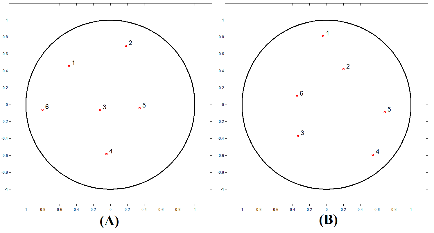
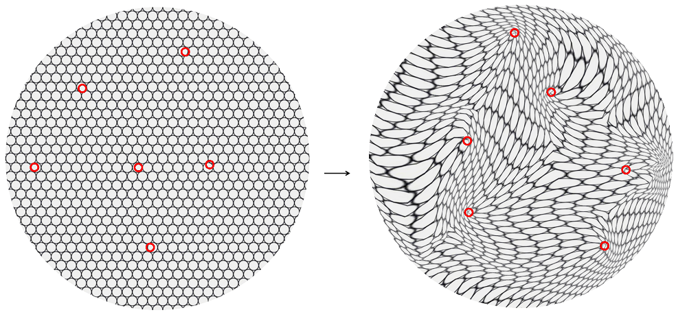
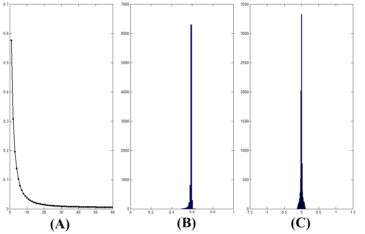
In our second example, we test our algorithm to compute the extremal Teichmuller map between two punctured unit disks. Figure 6(A) and (B) show two unit disks, each with 6 punctures. Denote the source domain by , and denote the target domain by . The boundary correspondence of is chosen to be the identity map. Using the QC iteration, we compute the extremal Teichmüller map such that and for . The obtained map is visualized using texture map as shown in Figure 7. The small circles on the source domain is mapped to small ellipses on the target domain with the same eccentricity. Figure 8(A) shows the energy versus each iterations in the QC iterations, where is the area of . The energy monotonically decreases to 0, which agrees with our theoretical finding. (B) shows the histogram of the norm of the Beltrami differential. It accumulates at 0.6, which illustrates that the obtained map is indeed a Teichmüller map. (C) shows the histogram of the Laplacian of . It accumulates at 0, meaning that the argument of is indeed harmonic.
Example 3
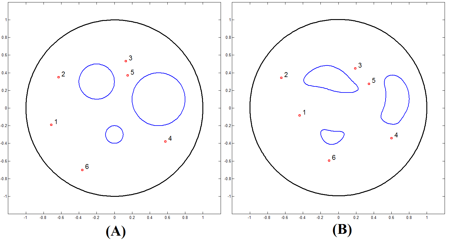
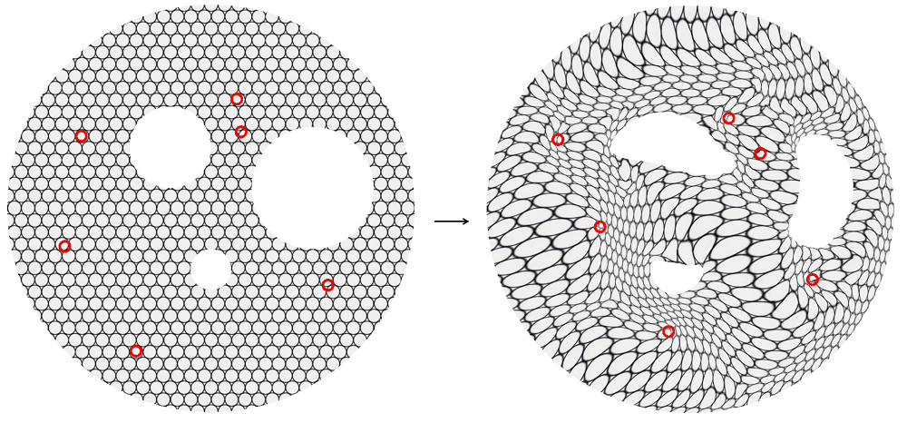
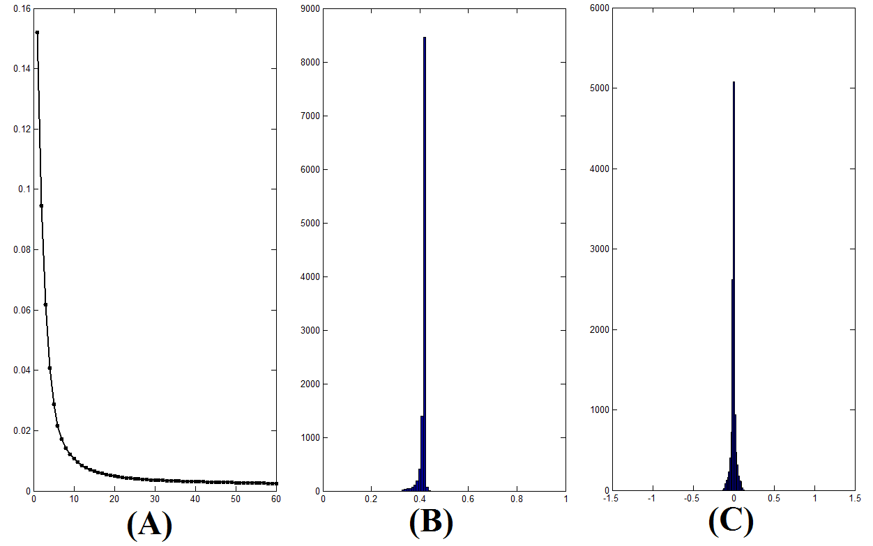
Finally, we test the QC iterations to compute the extremal Teichmüller map between two triply-connected domains and , each with 6 punctures. As shown in Figure 9(A), is chosen to be unit disk with three inner disks and six points removed (denote it by ). is chosen to be unit disk with three inner regions (with arbitrary shapes) and six points removed (denote it by ), as shown in (B). Again, the boundary correspondence is given. Using the QC iterations, we compute the extremal Teichmüller map such that and for . The obtained map is visualized using texture map as shown in Figure 10. The small circles on the source domain is mapped to small ellipses on the target domain with the same eccentricity. Figure 11(A) shows the energy versus each iterations in the QC iterations, where is the area of . The energy monotonically decreases to 0, which agrees with our theoretical finding. (B) shows the histogram of the norm of the Beltrami differential. It accumulates at 0.42, which illustrates that the obtained map is indeed a Teichmüller map. (C) shows the histogram of the Laplacian of . It accumulates at 0, meaning that the argument of is indeed harmonic.
6 Conclusion
This paper gives the convergence proof of the iterative algorithm proposed in [11] to compute the extremal Teichmüller map between Riemann surfaces of finite type. The iterative algorithm, which is named as quasi-conformal (QC) iteration, can be formulated as the optimization process of the harmonic energy. With this formulation, the QC iteration can be considered as the gradient descent of the harmonic energy under the auxiliary metric given by the Beltrami differentials.
In the future, we will further improve the efficiency of the iterative scheme to optimize the harmonic energy. The proposed framework will also be further extended to compute Teichmüller maps between high-genus surfaces (genus ).
References
- [1] A. Fletcher and V. Markovic Quasiconformal maps and Teichmüller theory. Oxford graduate text of mathematics, 11, 2007
- [2] S. Haker, S. Angenent, A. Tannenbaum, R. Kikinis, G. Sapiro, and M. Halle. Conformal surface parameterization for texture mapping, IEEE Transaction of Visualization and Computer Graphics, 6, 181-189, 2000.
- [3] B. Fischl, M. Sereno, R. Tootell, and A. Dale. High-resolution intersubject averaging and a coordinate system for the cortical surface. Human Brain Mapping, 8, 272-284, 1999.
- [4] X. Gu, Y. Wang, T. F. Chan, P. M. Thompson, and S.-T. Yau. Genus zero surface conformal mapping and its application to brain, surface mapping. IEEE Transactions on Medical Imaging, 23(8), 949-958, 2004.
- [5] Y. Wang, L. M. Lui, X. Gu, K. M. Hayashi, T. F. Chan, A. W. Toga, P. M. Thompson, and S.-T. Yau. Brain surface conformal parameterization using riemann surface structure. IEEE Transactions on Medical Imaging, 26(6), 853-865, 2007.
- [6] X. Gu and S. Yau. Computing conformal structures of surfaces, Communication in Information System, 2(2), 121-146, 2002.
- [7] M. K. Hurdal and K. Stephenson. Discrete conformal methods for cortical brain flattening, Neuroimage, 45, 86-98, 2009.
- [8] R.M. Porter An Interpolating Polynomial Method for Numerical Conformal Mapping. SIAM Journal on Scientific Computing, 23(3), 10271041, 2001
- [9] N. Hale and T.W. Tee Conformal Maps to Multiply-Slit Domains and Applications. SIAM Journal on Scientific Computing, 31(4), 3195-3215, 2009
- [10] T.K. DeLillo and E.H. Kropf Numerical Computation of the SchwarzChristoffel Transformation for Multiply Connected Domains. SIAM Journal on Scientific Computing, 33(3), 3195-3215, 2011
- [11] L.M. Lui, K.C. Lam, S.T. Yau, X.F. Gu Teichmüller extremal mapping and its applications to landmark matching registration. arXiv:1211.2569(http://arxiv.org/abs/1210.8025)
- [12] F. Gardiner and N. Lakic. Quasiconformal Teichmuller Theory. American Mathematics Society, 2000.
- [13] O. Lehto and K. Virtanen. Quasiconformal Mappings in the Plane. Springer-Verlag, New York, 1973.
- [14] Kurt Strebel. On Quasiconformal Mappings of Open Riemann Surfaces. Comment. Math. Helvetici, 53, 301-321, 1978.
- [15] Edgar Reich. Extremal Quasi-conformal Mappings of the Disk. Handbook of Complex Analysis: Geometric Function Theory, Vol 1, Chapter 3, 75-135, 2002.