1 \authorheadlineK. L. Ho and L. Ying \titleheadlineHIF-IE
Stanford University Stanford University
Hierarchical Interpolative Factorization for Elliptic Operators: Integral Equations
Abstract
This paper introduces the hierarchical interpolative factorization for integral equations (HIF-IE) associated with elliptic problems in two and three dimensions. This factorization takes the form of an approximate generalized LU decomposition that permits the efficient application of the discretized operator and its inverse. HIF-IE is based on the recursive skeletonization algorithm but incorporates a novel combination of two key features: (1) a matrix factorization framework for sparsifying structured dense matrices and (2) a recursive dimensional reduction strategy to decrease the cost. Thus, higher-dimensional problems are effectively mapped to one dimension, and we conjecture that constructing, applying, and inverting the factorization all have linear or quasilinear complexity. Numerical experiments support this claim and further demonstrate the performance of our algorithm as a generalized fast multipole method, direct solver, and preconditioner. HIF-IE is compatible with geometric adaptivity and can handle both boundary and volume problems. MATLAB codes are freely available.
1 Introduction
This paper considers integral equations (IEs) of the form
| (1) |
associated with elliptic partial differential equations (PDEs), where , , , and are given functions; the integral kernel is related to the fundamental solution of the underlying PDE; and or . Such equations encompass both boundary and volume problems and can be derived from PDEs in various ways. We give two prototypical examples below:
- 1.
Consider the interior Dirichlet Laplace problem
(2a) (2b) in a smooth, simply connected domain, which can be solved by writing as the double-layer potential
(3) over an unknown surface density , where
(4) is the fundamental solution of the free-space PDE and is the unit outer normal at . By construction, (3) satisfies (2a). To enforce the boundary condition (2b), take the limit as and use standard results from potential theory [31] to obtain
(5) where the integral is defined in the principal value sense. This is a boundary IE for of the form (1) (up to a straightforward generalization to matrix-valued kernels).
Alternatively, one could use the single-layer potential representation
which immediately gives the IE
upon taking the limit as since the integral is well-defined. Note that this has in (1). Such equations are called first-kind Fredholm IEs and are generally ill-conditioned. Second-kind Fredholm IEs such as (5), on the other hand, have for all and are usually well-conditioned.
- 2.
IEs can similarly be derived for many of the PDEs of classical physics including the Laplace, Helmholtz, Stokes, and time-harmonic Maxwell equations. In such cases, the kernel function is typically singular near zero but otherwise smooth with non-compact support. For this paper, we will also require that not be too oscillatory.
Discretization of (1) using, e.g., the Nyström, collocation, or Galerkin method leads to a linear system
| (6) |
where is dense with and the discrete analogues of and , respectively. This paper is concerned with the efficient factorization and solution of such systems.
1.1 Previous Work
Numerical methods for solving (6) can be classified into several groups. The first consists of classical direct methods like Gaussian elimination or other standard matrix factorizations [26], which compute the solution exactly (in principle, to machine precision, up to conditioning) without iteration. These methods are useful when is small. However, since is dense, such algorithms generally have complexity, which quickly makes them infeasible as increases.
The second group is that of iterative methods, among the most popular of which are Krylov subspace methods such as conjugate gradient [38, 49] or GMRES [47]. The number of iterations required depends on the problem and is typically small for second-kind IEs but can grow rapidly for first-kind ones. The main computational cost is the calculation of matrix-vector products at each iteration. Combined with fast multipole methods (FMMs) [22, 28, 29, 54] or other accelerated matrix multiplication schemes [5, 36], such techniques can yield asymptotically optimal or near-optimal solvers with or complexity. However, iterative methods are not as robust as their direct counterparts, especially when , , or lacks regularity or has high contrast. In such cases, convergence can be slow and specialized preconditioners are often needed. Furthermore, iterative methods can be inefficient for systems involving multiple right-hand sides or low-rank updates, which is an important setting for many applications of increasing interest, including time stepping, inverse problems, and design.
The third group covers rank-structured direct solvers, which exploit the observation that certain off-diagonal blocks of are numerically low-rank in order to dramatically lower the cost. The seminal work in this area is due to Hackbusch et al. [32, 34, 35], whose - and -matrices have been shown to achieve linear or quasilinear complexity. Although their work has had significant theoretical impact, in practice, the constants implicit in the asymptotic scalings tend to be large due to the recursive nature of the inversion algorithms and the use of expensive hierarchical matrix-matrix multiplication.
More recent developments aimed at improving practical performance include solvers for hierarchically semiseparable (HSS) matrices [10, 11, 51] and methods based on recursive skeletonization (RS) [25, 27, 39, 43], among other related schemes [2, 8, 13]. These can be viewed as special cases of -matrices and are optimal in one dimension (1D) (e.g., boundary IEs on curves) but have superlinear complexities in higher dimensions. In particular, RS proceeds analogously to the nested dissection multifrontal method (MF) for sparse linear systems [19, 23], with the so-called skeletons characterizing the off-diagonal blocks corresponding to the separator fronts. These grow as in two dimensions (2D) and in three dimensions (3D), resulting in solver complexities of and , respectively.
Recently, Corona, Martinsson, and Zorin [16] constructed an RS solver in 2D by exploiting further structure among the skeletons and using hierarchical matrix algebra. The principal observation is that for a broad class of integral kernels, the generic behavior of RS is to retain degrees of freedom (DOFs) only along the boundary of each cell in a domain partitioning. Thus, 2D problems are reduced to 1D, and the large skeleton matrices accumulated throughout the algorithm can be handled efficiently using 1D HSS techniques. However, this approach is quite involved and has yet to be realized in 3D or in complicated geometries.
1.2 Contributions
In this paper, we introduce the hierarchical interpolative factorization for IEs (HIF-IE), which produces an approximate generalized LU decomposition of with linear or quasilinear complexity estimates. HIF-IE is based on RS but augments it with a novel combination of two key features: (1) a matrix factorization formulation via a sparsification framework similar to that developed in [11, 50, 51] and (2) a recursive dimensional reduction scheme as pioneered in [16]. Unlike [16], however, which keeps large skeleton sets but works with them implicitly using fast structured methods, our sparsification approach allows us to reduce the skeletons explicitly. This obviates the need for internal hierarchical matrix representations, which substantially simplifies the algorithm and enables it to extend naturally to 3D and to complex geometries, in addition to promoting a more direct view of the dimensional reduction process.
Figure 1 shows a schematic of HIF-IE as compared to RS in 2D.

In RS (top), the domain is partitioned into a set of square cells at each level of a tree hierarchy. Each cell is skeletonized from the finest level to the coarsest, leaving DOFs only along cell interfaces. The size of these interfaces evidently grows as we march up the tree, which ultimately leads to the observed complexity.
In contrast, in HIF-IE (bottom), we start by skeletonizing the cells at the finest level as in RS but, before proceeding further, perform an additional level of edge skeletonization by grouping the remaining DOFs by cell edge. This respects the 1D structure of the interface geometry and allows more DOFs to be eliminated. The combination of cell and edge compression is then repeated up the tree, with the result that the skeleton growth is now suppressed. The reduction from 2D (square cells) to 1D (edges) to zero dimensions (0D) (points) is completely explicit. Extension to 3D is immediate by skeletonizing cubic cells, then faces, then edges at each level to execute a reduction from 3D to 2D to 1D to 0D. This tight control of the skeleton size is essential for achieving near-optimal scaling.
Once the factorization has been constructed, it can be used to rapidly apply both and , thereby serving as a generalized FMM, direct solver, or preconditioner (depending on the accuracy). Other capabilities are possible, too, though they will not be pursued here. As such, HIF-IE is considerably more general than many previous non–factorization-based fast direct solvers [10, 16, 25, 39, 43], which facilitate only the application of the inverse.
Extensive numerical experiments reveal strong evidence for quasilinear complexity and demonstrate that HIF-IE can accurately approximate various integral operators in both boundary and volume settings with high practical efficiency.
1.3 Outline
The remainder of this paper is organized as follows. In Section 2, we introduce the basic tools needed for our algorithm, including an efficient matrix sparsification operation that we call skeletonization. In Section 3, we describe the recursive skeletonization factorization (RSF), a reformulation of RS using our new factorization approach. This will serve to familiarize the reader with our sparsification framework as well as to highlight the fundamental difficulty associated with RS methods in 2D and 3D. In Section 4, we present HIF-IE as an extension of RSF with additional levels of skeletonization corresponding to recursive dimensional reductions. Although we cannot yet provide a rigorous complexity analysis, estimates based on well-supported rank assumptions suggest that HIF-IE achieves linear or quasilinear complexity. This conjecture is borne out by numerical experiments, which we detail in Section 5. Finally, Section 6 concludes with some discussion and future directions.
2 Preliminaries
In this section, we first list our notational conventions and then describe the basic elements of our algorithm.
Uppercase letters will generally denote matrices, while the lowercase letters , , , , and denote ordered sets of indices, each of which is associated with a DOF in the problem. For a given index set , its cardinality is written . The (unordered) complement of is given by , with the parent set to be understood from the context. The uppercase letter is reserved to denote a collection of disjoint index sets.
Given a matrix , is the submatrix with rows and columns restricted to the index sets and , respectively. We also use the MATLAB notation to denote the submatrix with columns restricted to .
Throughout, refers to the -norm.
2.1 Sparse Elimination
Let
| (7) |
be a matrix defined over the indices . This matrix structure often appears in sparse PDE problems, where, for example, corresponds to the interior DOFs of a region , to the DOFs on the boundary , and to the external region , which should be thought of as large. In this setting, the DOFs and are separated by and hence do not directly interact, resulting in the form (7).
Our first tool is quite standard and concerns the efficient elimination of DOFs from such sparse matrices.
Lemma 2.1
Let be given by (7) and write in factored form, where and are unit triangular matrices (up to permutation). If is nonsingular, then
| (8) |
where
and is the associated Schur complement.
Note that the indices have been decoupled from the rest. Regarding the subsystem in (8) over the indices only, we may therefore say that the DOFs have been eliminated. The operators and carry out this elimination, which furthermore is particularly efficient since the interactions involving the large index set are unchanged.
2.2 Interpolative Decomposition
Our next tool is the interpolative decomposition (ID) [14] for low-rank matrices, which we present in a somewhat nonstandard form below.
Lemma 2.2
Let with rank . Then there exist a partitioning with and a matrix such that .
Proof.
Let
be a so-called thin pivoted QR decomposition of , where is unitary, is upper triangular, and the permutation matrix has been chosen so that is nonsingular. Then identifying the first pivots with and the remainder with ,
for . ∎
The ID can also be written more traditionally as
where is the permutation matrix associated with the ordering . We call and the skeleton and redundant indices, respectively. Lemma 2.2 states that the redundant columns of can be interpolated from its skeleton columns. The following shows that the ID can also be viewed as a sparsification operator.
Corollary 2.3
Let be a low-rank matrix. If and are such that , then
In general, let for some error matrix and characterize the ID by the functions and such that
| (9) |
where is the st largest singular value of . If and are not too large, then (9) implies that the reconstruction of is stable and accurate. There exists an ID with
| (10) |
for , but computing it can take exponential time, requiring the combinatorial maximization of a submatrix determinant. However, an ID satisfying (10) with any can be computed in polynomial time [30]. In this paper, we use the algorithm of [14] based on a simple pivoted QR decomposition, which has a possibility of failure but seems to consistently achieve (10) with in practice at a cost of operations. Fast algorithms based on random sampling are also available [37], but these can incur some loss of accuracy (see also Section 4.3).
The ID can be applied in both fixed and adaptive rank settings. In the former, the rank is specified, while, in the latter, the approximation error is specified and the rank adjusted to achieve (an estimate of) it. Hereafter, we consider the ID only in the adaptive sense, using the relative magnitudes of the pivots to adaptively select such that for any specified relative precision .
2.3 Skeletonization
We now combine Lemmas 2.1 and 2.2 to efficiently eliminate redundant DOFs from dense matrices with low-rank off-diagonal blocks.
Lemma 2.4
Let
with and low-rank, and let and be such that
i.e., and . Without loss of generality, write
and define
Then
| (11) |
where
so
| (12) |
where and are the elimination operators of Lemma 2.1 associated with and , assuming that is nonsingular.
In essence, the ID sparsifies by decoupling from , thereby allowing it to be eliminated using efficient sparse techniques. We refer to this procedure as skeletonization since only the skeletons remain. Note that the interactions involving are unchanged. A very similar approach has previously been described in the context of HSS ULV decompositions [11] by combining the structure-preserving rank-revealing factorization [53] with reduced matrices [50].
In general, the ID often only approximately sparsifies (for example, if its off-diagonal blocks are low-rank only to a specified numerical precision) so that (11) and consequently (12) need not hold exactly. In such cases, the skeletonization operator should be interpreted as also including an intermediate truncation step that enforces sparsity explicitly. For notational convenience, however, we will continue to identify the left- and right-hand sides of (12) by writing , with the truncation to be understood implicitly.
In this paper, we often work with a collection of disjoint index sets, where and are numerically low-rank for all . Applying Lemma 2.4 to all gives
where the redundant DOFs for each have been decoupled from the rest and the matrix products over can be taken in any order. The resulting skeletonized matrix is significantly sparsified and has a block diagonal structure over the index groups
where the outer union is to be understood as acting on collections of index sets and is the set of all indices.
3 Recursive Skeletonization Factorization
In this section, we present RSF, a reformulation of RS [25, 27, 39, 43] as a matrix factorization using the sparsification view of skeletonization as developed in Lemma 2.4. Mathematically, RSF is identical to RS but expresses the matrix as a (multiplicative) multilevel generalized LU decomposition instead of as an additive hierarchical low-rank update. This representation enables much simpler algorithms for applying and as well as establishes a direct connection with MF [19, 23] for sparse matrices, which produces a (strict) LU decomposition using Lemma 2.1. Indeed, RSF is essentially just MF with pre-sparsification via the ID at each level. This point of view places methods for structured dense and sparse matrices within a common framework, which provides a potential means to transfer techniques from one class to the other.
Note that because RSF is based on elimination, it requires that certain intermediate matrices be invertible, which in general means that must be square. This is a slight limitation when compared to RS, which can be used, for example, as a generalized FMM [25, 39] or least squares solver [40] for rectangular matrices.
We begin with a detailed description of RSF in 2D before extending to 3D in the natural way (the 1D case will not be treated but should be obvious from the discussion). The same presentation framework will also be used for HIF-IE in Section 4, which we hope will help make clear the specific innovations responsible for its improved complexity estimates.
3.1 Two Dimensions
Consider the IE (1) on , discretized using a piecewise constant collocation method over a uniform grid for simplicity. More general domains and discretizations can be handled without difficulty, but the current setting will serve to illustrate the main ideas. Let be the step size in each direction and assume that , where is a small integer. Integer pairs index the elements and their centers for . With as the collocation points, the discrete system (6) reads
at each , where , , , and ; is the approximation to ; and
| (13) |
Note that is not stored since it is dense; rather, its entries are generated as needed. The total number of DOFs is , each of which is associated with a point and an index in .
The algorithm proceeds by eliminating DOFs level by level. At each level , the set of DOFs that have not been eliminated are called active with indices . Initially, we set and . Figure 2 shows the active DOFs at each level for a representative example.


Level
Defined at this stage are and . Partition into the Voronoi cells [4] of width about the centers for . Let be the collection of index sets corresponding to the active DOFs of each cell. Clearly, . Then skeletonization with respect to gives
where the DOFs have been eliminated (and marked inactive). Let be the remaining active DOFs. The matrix is block diagonal with block partitioning
Level
Defined at this stage are and . Partition into the Voronoi cells of width about the centers for . Let be the collection of index sets corresponding to the active DOFs of each cell. Clearly, . Skeletonization with respect to then gives
where the DOFs have been eliminated. The matrix is block diagonal with block partitioning
where .
Level
Finally, we have and , where is block diagonal with block partitioning
Combining the approximation over all levels gives
where each and are products of unit triangular matrices, each of which can be inverted simply by negating its off-diagonal entries. Therefore,
| (14a) | ||||
| (14b) | ||||
The factorization permits fast multiplication and can be used as a generalized FMM. Its inverse can be used as a direct solver at high accuracy or as a preconditioner otherwise. If is stored in factored form, e.g., as an LU decomposition, then the same factorization can readily be used for both tasks. We call (14) an (approximate) generalized LU decomposition since while each and are composed of triangular factors, they are not themselves triangular, being the product of both upper and lower triangular matrices. We emphasize that and are not assembled explicitly and are applied only in factored form.
The entire procedure is summarized compactly as Algorithm 3.1. In general, we construct the cell partitioning at each level using an adaptive quadtree [48], which recursively subdivides the domain until each node contains only DOFs.
3.2 Three Dimensions
Consider now the analogous setting in 3D, where is discretized using a uniform grid with and for . The total number of DOFs is .
The algorithm extends in the natural way with cubic cells about the centers replacing the square cells in 2D at level for . With this modification, the rest of the algorithm remains unchanged. Figure 3 shows the active DOFs at each level for a representative example.


The output is again a factorization of the form (14). General geometries can be treated using an adaptive octree.
3.3 Accelerated Compression
A dominant contribution to the cost of RSF is computing IDs for skeletonization. The basic operation required is the construction of an ID of
where and , following Lemma 2.4. We hereafter drop the dependence on for notational convenience. Observe that is a tall-and-skinny matrix of size , so forming its ID takes at least work. The total number of index sets for all is , so considering all yields a lower bound of on the total work and hence on the complexity of RSF.
In principle, it is straightforward to substantially accelerate the algorithm by reconstructing an ID of from that of a much smaller matrix . All that is needed is that the rows of span those of , i.e., , where denotes the matrix range.
Lemma 3.1
Let with column indices . If and are such that , then
In other words, an ID of gives an ID of . Note that we make no explicit reference to ; only its existence is assumed. Of course, such a small matrix always exists since ; the difficulty lies in finding a priori.
For elliptic problems, the integral kernel typically satisfies some form of Green’s theorem, in which its values inside a region can be recovered from its values on the boundary . Consider, for example, the Laplace kernel (4) and let be the harmonic field in due to an exterior source . Then
i.e., the “incoming” field lives in the span of single- and double-layer interactions with . In practice, we will use this fact only when is sufficiently separated from (see below), in which case the double-layer term can often even be omitted since the corresponding discrete spaces are equal to high precision. Outgoing interactions can essentially be treated in the same way using the “transpose” of this idea.
In such cases, a suitable can readily be constructed. To see this, let denote the cell containing the DOFs and draw a local “proxy” surface around (Figure 4).

This partitions as , where consists of all DOFs interior to (the near field) and consists of the rest (the far field). By Green’s theorem, the interactions involving can be represented by artificial “equivalent” interactions with . Therefore, discretizing with equivalent DOFs , we assert that:
Lemma 3.2
Proof.
This immediately follows from Green’s theorem upon recognizing that contains interactions involving only the original kernel function . This must be checked because may have Schur complement interactions (SCIs), i.e., those corresponding to the matrix in (12), accumulated from skeletonization at previous levels, over which we do not have analytic control. However, due to the hierarchical nature of the domain partitioning, any such SCIs must be restricted to the diagonal block . Thus, Green’s theorem applies. ∎
Lemma 3.3
Consider (1) with general and . Then, up to discretization error, and , where
Proof.
If is separated from , for example as in Figure 4, then standard multipole estimates [28, 29] show that we only need to satisfy Green’s theorem to any precision . In particular, for fixed , we can choose to be constant. Therefore, Lemma 3.3 gives
| (15) |
for some , where has size with typically. Lemma 3.1 then reduces the global compression of to the local compression of . This so-called proxy trick has also been employed by [14, 16, 25, 27, 39, 43, 44, 46, 54] and is crucial for reducing the asymptotic complexity. For numerical stability, we include the quadrature weights for the integral (13) in and so that the various components of are all of the same order.
In this paper, for a cell with scaled width centered at the origin, we take as the circle of radius in 2D, uniformly discretized with points, and the sphere of radius in 3D, uniformly sampled (by projecting Gaussian random vectors) with points. These values of have been experimentally validated to reproduce interactions via the Laplace kernel (4) with . This approach is more efficient than the “supercell” proxy of [27, 39] by factors of in 2D and in 3D (volume ratio of the cube to the sphere of equal diameter), which takes as the outer boundary of the () cell block centered at .
3.4 Complexity Estimates
We now investigate the computational complexity of RSF. For this, we need to estimate the skeleton size for a typical index set at level . Denote this quantity by and let be the number of DOFs (both active and inactive) in each cell. From Figures 2 and 3, it is clear that skeletons tend to cluster around cell interfaces, which can again be justified by Green’s theorem, so in 2D and in 3D. Indeed, this can be verified using standard multipole estimates by noting that is on the order of the interaction rank between two adjacent cells at level , which can be analyzed via recursive subdivision to expose well-separated structures (Figure 5).

This yields the more detailed result
| (16) |
which, in fact, holds for equal to the intrinsic dimension rather than the ambient dimension.
Proof.
Consider first the factorization cost . There are cells at level , where each cell requires the calculation of an ID of in (15) as well as various local matrix operations at a total cost of , assuming that . But for , while for since the active DOFs are obtained by merging the skeletons of cells at level . Hence, (17) follows.
A similar derivation holds for by observing that each requires local matrix-vector products with cost . ∎
Remark 3.5.
If a tree is used, then there is also a cost of for tree construction, but the associated constant is tiny and so we can ignore it for all practical purposes.
The memory cost to store itself is clearly and so is also given by (18). From Theorem 3.4, it is immediate that RSF behaves just like MF, with the geometric growth of in 2D and 3D leading to suboptimal complexities.
Corollary 3.6
If
| (19) |
for some constant , then and .
Proof.
From (17), , so choosing gives and . Similarly, . ∎
This is a more precise version of the 1D result that will be useful later when discussing HIF-IE.
4 Hierarchical Interpolative Factorization
In this section, we present HIF-IE, which builds upon RSF by introducing additional levels of skeletonization in order to effectively reduce all problems to 1D. Considering the 2D case for concreteness, the main idea is simply to employ an additional level after each level by partitioning according to the cell edges near which the surviving active DOFs cluster. This fully exploits the 1D geometry of the active DOFs. However, the algorithm is complicated by the fact that the cell and edge partitions are non-nested, so different index groups may now interact via SCIs. Such SCIs do not lend themselves easily to analysis and we have yet to prove a statement like (16) on their ranks. Nevertheless, extensive numerical experiments by ourselves (Section 5) and others [16] reveal that very similar bounds appear to be obeyed. This suggests that SCIs do not need to be treated in any significantly different way, and we hereafter assume that interaction rank is completely determined by geometry.
The overall approach of HIF-IE is closely related to that of [16], but our sparsification framework permits a much simpler implementation and analysis. As with RSF, we begin first in 2D before extending to 3D.
4.1 Two Dimensions
Assume the same setup as in Section 3.1. HIF-IE supplements cell skeletonization (2D to 1D) at level with edge skeletonization (1D to 0D) at level for each . Figure 6 shows the active DOFs at each level for a representative example.


Level
Partition into Voronoi cells about the cell centers for . Let be the collection of index sets corresponding to the active DOFs of each cell. Skeletonization with respect to then gives
where the DOFs have been eliminated.
Level
Partition into Voronoi cells about the edge centers for , and for , . Let be the collection of index sets corresponding to the active DOFs of each cell. Skeletonization with respect to then gives
where the DOFs have been eliminated.
Level
Combining the approximation over all levels gives
so
| (20a) | ||||
| (20b) | ||||
This is a factorization of exactly the same type as that in (14) (but with twice the number of factors). The entire procedure is summarized as Algorithm 4.1.
4.2 Three Dimensions
Assume the same setup as in Section 3.2. HIF-IE now performs two rounds of additional dimensional reduction over RSF by supplementing cell skeletonization (3D to 2D) at level with face skeletonization (2D to 1D) at level and edge skeletonization (1D to 0D) at level . Figure 7 shows the active DOFs at each level for a representative example.


Level
Partition into Voronoi cells about the cell centers for . Let be the collection of index sets corresponding to the active DOFs of each cell. Skeletonization with respect to then gives
where the DOFs have been eliminated.
Level
Partition into Voronoi cells about the face centers
Let be the collection of index sets corresponding to the active DOFs of each cell. Skeletonization with respect to then gives
where the DOFs have been eliminated.
Level
Partition into Voronoi cells about the edge centers
Let be the collection of index sets corresponding to the active DOFs of each cell. Skeletonization with respect to then gives
where the DOFs have been eliminated.
Level
Combining the approximation over all levels gives
so
| (21a) | ||||
| (21b) | ||||
This procedure is summarized as Algorithm 4.2.
4.3 Accelerated Compression
Proxy compression still applies, provided that we make some minor modifications to account for SCIs, which we generally have access to only numerically and so cannot evaluate at arbitrary points as needed in Lemma 3.3. Specifically, for a given index set , we now expand by including all DOFs that interact with via SCIs in addition to those interior to as in Section 3.3. The far field then consists only of original kernel interactions, so Lemma 3.3 holds. It remains to observe that SCIs are local due to the domain partitioning strategy. Thus, all reside in an immediate neighborhood of and we again conclude that .
Even with this acceleration, however, the ID still manifests as a computational bottleneck. To combat this, we also tried fast randomized methods [37] based on compressing , where is a small Gaussian random sampling matrix. We found that the resulting ID was inaccurate when contained SCIs. This could be remedied by considering instead for some small integer , but the expense of the extra multiplications usually outweighed any efficiency gains.
4.4 Modifications for Second-Kind Integral Equations
The algorithms presented so far are highly accurate for first-kind IEs in that , where is the input precision to the ID (Section 5). For second-kind IEs, however, we see a systematic deterioration of the relative error roughly as as . This instability can be explained as follows. Let be a typical second-kind IE matrix discretization. Then the diagonal entries of are , while its off-diagonal entries are . Since the interpolation matrix, say, from the ID has entries of order , the same is true of , , and in (11). Therefore, the entries of the Schur complement in (12) are , i.e., SCIs dominate kernel interactions by a factor of .
Lemma 4.1
Assume the setting of the discussion above and let be such that in (15) contains SCIs. Then , so the ID of has absolute error .
Consider now the process of “unfolding” the factorization from the middle matrix outward. This is accomplished by undoing the skeletonization operation for each in reverse order, at each step reconstructing and from and . Restricting attention to 2D for concreteness, we start at level with interactions between the DOFs as depicted in Figure 8 (left).

By Lemma 4.1, un-skeletonizing each edge induces an error in the interactions between the edges and as labeled in the figure (center) of absolute magnitude . At the next level, un-skeletonizing the shaded cell which they bound then relies on the approximate interactions between and . This spreads the error over the reconstructed cell interactions, which is small for SCIs acting internally to each cell (omitting level for simplicity) but not for kernel interactions between any two distinct cells and (right); indeed, the relative error for the latter is . These corrupted interactions are then used for reconstruction at the next level and are eventually spread throughout the whole matrix. The same argument clearly holds in 3D.
This analysis suggests that the only fix is to skeletonize at effective precision so that kernel interactions are accurately reconstructed. This is equivalent to ensuring that both scales in are well approximated by the ID. Following this intuition, we decompose as , where consists purely of kernel interactions, and set for as the local compression tolerance, which we note uses increased precision only when necessary.
The two-scale structure of also enables an additional optimization as can be seen by studying the sparsity patterns of SCIs. Figure 9 shows an example configuration in 2D after cell skeletonization at level , which leaves a collection of edges at level , each composed of two half-edges consisting of skeletons from the two cells on either side (left).
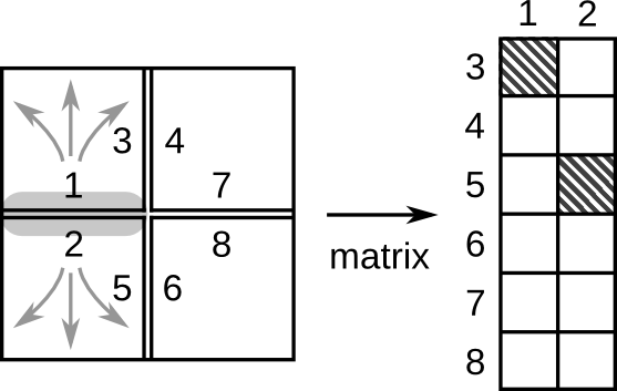
Let be a given edge with indices partitioned by half-edge, and let be the submatrix of corresponding to . Then and (analogously defined) have different nonzero structures, so and have large entries in different row blocks (right). The stable interpolation of hence requires that all interpolation coefficients from one half-edge to the other be since otherwise the reconstruction of, say, will have large errors in rows where is nonzero. As , these cross-interpolation coefficients must therefore vanish and the compression of decouples into the compression of and separately. We enforce this asymptotic decoupling explicitly, which moreover provides an acceleration due to the cubic cost of the ID. The ID of is then given by , , and , where and define the ID of . We use the compression tolerance with locally for each .
In general, we define the subsets algebraically according to the sparsity pattern of , which can be done using the matrix indicator function
Lemma 4.2
Let for some matrix . Then and have the same sparsity pattern if and only .
4.5 Complexity Estimates
Analysis of HIF-IE is impeded by the compression of SCIs, for which we do not have rigorous bounds on the interaction rank. Nonetheless, ample numerical evidence suggests that SCIs behave very similarly to standard kernel interactions. For the sake of analysis, we hence assume that the same rank estimates apply, from which we have (19) for all by reduction to 1D. We emphasize that this has yet to be proven, so all following results should formally be understood as conjectures, albeit ones with strong experimental support (Section 5).
Theorem 4.3
Proof.
This is essentially just a restatement of Corollary 3.6 (but with the sum now taken also over fractional levels). ∎
Corollary 4.4
For second-kind IEs,
Proof.
According to the modifications of Section 4.4, there are now two effective ID tolerances: for all such that and otherwise. The former is used for all initial levels before SCIs have become widespread (i.e., before any meaningful dimensional reduction has occurred), and the latter for all . But using precision yields a rank estimate with constant of proportionality , where is the intrinsic dimension of the DOF cluster [28, 29], so the amount of compression depends on . Thus, and our first task is to determine its form.
The crossover level can be obtained by balancing the typical size of an edge (2D and 3D) or face (3D only) with its skeleton size . In 2D, this is , where the left-hand side gives the size of an edge at level , and the right-hand side the estimated rank for SCI compression. Therefore, .
In 3D, there are two crossover levels and corresponding to face and edge compression, respectively, with :
Hence, and , so .
The cost of constructing for second-kind IEs is then
where prime notation denotes summation over all levels, both integer and fractional, and is as given in (19) with . The first sum corresponds to running RSF on the initial levels and reduces to
while the second can be interpreted as the cost of the standard HIF-IE (without modification) applied to the remaining
DOFs at uniform precision . By Corollary 3.6, this is
so, adding all terms, we derive as claimed.
A similar argument for
completes the proof. ∎
5 Numerical Results
In this section, we demonstrate the efficiency of HIF-IE by reporting numerical results for some benchmark problems in 2D and 3D. All algorithms and examples were implemented in MATLAB and are freely available at https://github.com/klho/FLAM/. In what follows, we refer to RSF as rskelf2 in 2D and rskelf3 in 3D. Similarly, we call HIF-IE hifie2 and hifie3, respectively, with hifie2x and hifie3x denoting their second-kind IE counterparts. All codes are fully adaptive and built on quadtrees in 2D and octrees in 3D. The average block size at level (and hence the tree depth ) was chosen so that . In select cases, the first few fractional levels of HIF-IE were skipped to optimize the running time. Symmetry was exploited wherever possible by compressing
instead of the full matrix in (15), which reduces the cost by about a factor of . Diagonal blocks, i.e., in Lemma 2.1, were factored using the (partially pivoted) LDL decomposition if is symmetric and the LU decomposition otherwise.
For each example, the following, if applicable, are given:
- •
: base relative precision of the ID;
- •
: total number of DOFs in the problem;
- •
: number of active DOFs remaining at the highest level;
- •
: wall clock time for constructing the factorization in seconds;
- •
: memory required to store in GB;
- •
: wall clock time for applying or in seconds;
- •
: a posteriori estimate of (see below);
- •
: a posteriori estimate of ;
- •
: number of iterations to solve (6) using GMRES with preconditioner to a tolerance of , where is a standard uniform random vector (ill-conditioned systems only).
The operator errors and were estimated using power iteration with a standard uniform random start vector [18, 42] and a convergence criterion of relative precision in the matrix norm. This procedure requires the application of both and , which for translation-invariant kernels was done using fast Fourier convolution [9] and for non–translation-invariant kernels using an ID-based kernel-independent FMM [44, 46] at precision . The same methods were also used to apply when solving (6) iteratively.
For simplicity, all IEs were discretized using a piecewise constant collocation method as in Section 3. Certain near-field interactions (to be defined for each case) were computed using adaptive quadrature, while all other interactions were handled as simple one-point approximations, e.g., in (13).
All computations were performed in MATLAB R2010b on a single core (without parallelization) of an Intel Xeon E7-4820 CPU at 2.0 GHz on a 64-bit Linux server with 256 GB of RAM.
5.1 Two Dimensions
We begin first in 2D, where we present three examples.
Example 1
Consider (1) with , , , and , i.e., a first-kind volume IE in the unit square, discretized over a uniform grid. The diagonal entries are computed adaptively, while all for are approximated using one-point quadratures. We factored the resulting matrix using both rskelf2 and hifie2 at , , and . The data are summarized in Tables 1 and 2 with scaling results shown in Figure 10.
| rskelf2 | hifie2 | ||||||
|---|---|---|---|---|---|---|---|
| e | e | e | e | ||||
| e | e | e | e | ||||
| e | e | e | e | ||||
| e | e | e | e | ||||
| e | e | e | e | ||||
| e | e | e | e | ||||
| e | e | e | e | ||||
| e | e | e | e | ||||
| e | e | e | e | ||||
| rskelf2 | hifie2 | |||||
|---|---|---|---|---|---|---|
| e | e | e | e | |||
| e | e | e | e | |||
| e | e | e | e | |||
| e | e | e | e | |||
| e | e | e | e | |||
| e | e | e | e | |||
| e | e | e | e | |||
| e | e | e | e | |||
| e | e | e | e | |||

It is evident that behaves as predicted, with HIF-IE achieving significant compression over RSF. Consequently, we find strong support for asymptotic complexities consistent with Theorems 3.4 and 4.3. For all problem sizes tested, and are always smaller for HIF-IE, though is quite comparable. This is because is dominated by memory access (at least in our current implementation), which also explains its relative insensitivity to . Furthermore, we observe that for both methods, which makes them ideally suited to systems involving multiple right-hand sides.
The forward approximation error for all and seems to increase only very mildly, if at all, with . This indicates that the local accuracy of the ID provides a good estimate of the overall accuracy of the algorithm, which is not easy to prove since the multilevel matrix factors constituting are not unitary. On the other hand, we expect the inverse approximation error to scale as , where is the condition number of , and indeed we see that is much larger due to the ill-conditioning of the first-kind system. When using to precondition GMRES, however, the number of iterations required is always very small. This indicates that is a highly effective preconditioner.
Example 2
Consider now the same setup as in Example 1 but with . This gives a well-conditioned second-kind IE, which we factored using rskelf2, hifie2, and hifie2x. The data are summarized in Tables 3 and 4 with scaling results in Figure 11.
| rskelf2 | hifie2 | hifie2x | ||||||||
|---|---|---|---|---|---|---|---|---|---|---|
| e | e | e | e | e | e | |||||
| e | e | e | e | e | e | |||||
| e | e | e | e | e | e | |||||
| e | e | e | e | e | e | |||||
| e | e | e | e | e | e | |||||
| e | e | e | e | e | e | |||||
| e | e | e | e | e | e | |||||
| e | e | e | e | e | e | |||||
| e | e | e | e | e | e | |||||
| rskelf2 | hifie2 | hifie2x | ||||||
|---|---|---|---|---|---|---|---|---|
| e | e | e | e | e | e | e | ||
| e | e | e | e | e | e | e | ||
| e | e | e | e | e | e | e | ||
| e | e | e | e | e | e | e | ||
| e | e | e | e | e | e | e | ||
| e | e | e | e | e | e | e | ||
| e | e | e | e | e | e | e | ||
| e | e | e | e | e | e | e | ||
| e | e | e | e | e | e | e | ||

As expected, results for rskelf2 are essentially the same as those in Example 1 since the off-diagonal interactions at each level are identical. We also see the breakdown of hifie2, which still has linear complexity but fails to properly approximate as predicted in Section 4.4. This is remedied by hifie2x, which achieves but with a slight increase in cost. In particular, it appears to scale somewhat faster than linearly but remains consistent with Corollary 4.4.
Example 3
We then turn to the Lippmann-Schwinger equation
for Helmholtz scattering, where is the frequency of the incoming wave with the number of wavelengths in ; is the fundamental solution of the associated Helmholtz equation satisfying the Sommerfeld radiation condition, where is the imaginary unit and is the zeroth order Hankel function of the first kind; and is a continuous function representing the scatterer. We refer the interested reader to [15] for details. Assuming that , this can be symmetrized by the change of variables as
| (22) |
i.e., (1) with and . We took a Gaussian bump for as the scatterer and discretized (22) using a uniform grid with quadratures as computed in Example 1. The frequency was increased with to keep the number of DOFs per wavelength fixed at . Data for rskelf2, hifie2, and hifie2x with , , and at are shown in Tables 5 and 6.
| rskelf2 | hifie2 | hifie2x | |||||||||
|---|---|---|---|---|---|---|---|---|---|---|---|
| e | e | e | e | e | e | ||||||
| e | e | e | e | e | e | ||||||
| e | e | e | e | e | e | ||||||
| rskelf2 | hifie2 | hifie2x | |||||||||
|---|---|---|---|---|---|---|---|---|---|---|---|
| e | e | e | e | e | e | e | |||||
| e | e | e | e | e | e | e | |||||
| e | e | e | e | e | e | e | |||||
Overall, the results are similar to those in Example 2 but with added computational expense due to working over and computing . Moreover, although (22) is formally a second-kind IE, it becomes increasingly first-kind as . Thus, the problem is somewhat ill-conditioned, as reflected in the deterioration of and even for hifie2x. Nevertheless, remains a very good preconditioner, with for hifie2x. Interestingly, despite its inaccuracy, hifie2 is also quite effective for preconditioning: experimentally, we observe that , which can be justified as follows.
Lemma 5.1
If with , then the number of iterations for GMRES to solve (6) to any target precision is .
Proof.
Let be the th iterate with residual . Then the relative residual satisfies
where is the set of all polynomials of degree at most such that [47]. Consider, in particular, the choice . Then , so . Setting the left-hand side equal to yields . ∎
Corollary 5.2
Let and with and for some constant such that . Then the number of iterations for GMRES to solve (6) with preconditioner is
Proof.
The preconditioned matrix is , where
so Lemma 5.1 gives
But , so . The claim now follows by first-order expansion of the term in parentheses. ∎
We remark that HIF-IE is effective only at low to moderate frequency since the rank structures employed break down as . In the limit, the only compression possible is due to Green’s theorem, with HIF-IE reducing to RSF for volume IEs. The situation is yet worse for boundary IEs, for which no compression at all is available in general, and both RSF and HIF-IE revert to having complexity.
5.2 Three Dimensions
We next present three examples in 3D: a boundary IE and two volume IEs as in Examples 1 and 2.
Example 4
Consider the second-kind boundary IE (5) on the unit sphere , where is as defined in (4). It is possible to reparametrize in 2D and then use 2D algorithms, but we ran the full 3D solvers here. We represented as a collection of flat triangles and discretized via a centroid collocation scheme. Near-field interactions for all centroids within a local neighborhood of radius about each triangle, where is the average triangle diameter, were computed using fourth-order tensor-product Gauss-Legendre quadrature. This gives a linear system (6) with unsymmetric . Data for rskelf3, hifie3, and hifie3x at and are shown in Tables 7 and 8 with scaling results in Figure 12.
| rskelf3 | hifie3 | hifie3x | ||||||||
|---|---|---|---|---|---|---|---|---|---|---|
| e | e | e | e | e | e | |||||
| e | e | e | e | e | e | |||||
| e | e | e | e | e | e | |||||
| e | e | e | e | e | e | |||||
| e | e | e | e | e | e | |||||
| e | e | e | e | e | e | |||||
| e | e | e | e | e | e | |||||
| rskelf3 | hifie3 | hifie3x | ||||||
|---|---|---|---|---|---|---|---|---|
| e | e | e | e | e | e | e | ||
| e | e | e | e | e | e | e | ||
| e | e | e | e | e | e | e | ||
| e | e | e | e | e | e | e | ||
| e | e | e | e | e | e | e | ||
| e | e | e | e | e | e | e | ||
| e | e | e | e | e | e | e | ||

Since is a 2D surface, in Theorem 3.4, so we can expect RSF to have complexity, as observed. However, the skeleton size is substantially larger than in 2D, so the corresponding costs are much higher. The same is true for HIF-IE, which achieves quasilinear complexity as predicted in Theorem 4.3 and Corollary 4.4. As before, for hifie3x but suffer for hifie3.
We also tested the accuracy of our algorithms in solving the associated PDE (2) by constructing an interior harmonic field
due to random exterior sources with , where the “charge” strengths were drawn from the standard uniform distribution. This induces the boundary data , which returns the charge density upon solving (5). The field due to via the double-layer potential (3) is then, in principle, identical to by uniqueness of the boundary value problem. This equality was assessed by evaluating both and at random interior targets with . The relative error between and is shown in Table 9, from which we observe that rskelf3 and hifie3x are both able to solve the PDE up to the discretization or approximation error.
| rskelf3 | hifie3 | hifie3x | ||
|---|---|---|---|---|
| e | e | e | ||
| e | e | e | ||
| e | e | e | ||
| e | e | e | ||
| e | e | e | ||
| e | e | e | ||
| e | e | e |
Example 5
Now consider the 3D analogue of Example 1, i.e., (1) with , , , and , discretized over a uniform grid with adaptive quadratures for the diagonal entries. Data for rskelf3 and hifie3 at and are given in Tables 10 and 11 with scaling results in Figure 13.
| rskelf3 | hifie3 | ||||||
| e | e | e | e | ||||
| e | e | e | e | ||||
| — | — | — | e | e | |||
| e | e | e | e | ||||
| — | — | — | e | e | |||
| rskelf3 | hifie3 | |||||
| e | e | e | e | |||
| e | e | e | e | |||
| — | e | e | e | |||
| e | e | e | e | |||
| — | e | e | e | |||

It is immediate that and for RSF, which considerably degrades its performance for large . Indeed, we were unable to run rskelf3 for because of the excessive memory cost. In contrast, HIF-IE scales much better though does not quite achieve complexity as stated in Theorem 4.3: the empirical scaling for at , for instance, is approximately . We believe this to be a consequence of the large interaction ranks in 3D, which make the asymptotic regime rather difficult to reach. Still, even the experimental growth rate of would be sufficient for theoretical complexity. In parallel with Example 1, but is somewhat larger due to ill-conditioning. We found to be a very effective preconditioner throughout.
Example 6
Finally, we consider the 3D analogue of Example 2, i.e., Example 5 but with . This is a well-conditioned second-kind IE, which we factored using rskelf3, hifie3, and hifie3x. The data are summarized in Tables 12 and 13 with scaling results shown in Figure 14.
| rskelf3 | hifie3 | hifie3x | ||||||||
| e | e | e | e | e | e | |||||
| e | e | e | e | e | e | |||||
| — | — | — | e | e | e | e | ||||
| e | e | e | e | e | e | |||||
| — | — | — | e | e | e | e | ||||
| rskelf3 | hifie3 | hifie3x | ||||||
|---|---|---|---|---|---|---|---|---|
| e | e | e | e | e | e | e | ||
| e | e | e | e | e | e | e | ||
| — | e | e | e | e | e | e | ||
| e | e | e | e | e | e | e | ||
| — | e | e | e | e | e | e | ||

Algorithms rskelf3 and hifie3 behave very similarly as in Example 5 but with some error propagation for hifie3 as discussed in Section 4.4. Full accuracy is restored using hifie3x but at the cost of significantly larger skeleton sizes. The empirical complexity of hifie3x hence suffers but remains quite favorable compared to that of rskelf3. We also find a good fit with the complexity estimates of Corollary 4.4, though the presumed penalty for not yet reaching the asymptotic regime may imply that the proposed bounds are overly pessimistic.
6 Generalizations and Conclusions
In this paper, we have introduced HIF-IE for the efficient factorization of discretized integral operators associated with elliptic PDEs in 2D and 3D. HIF-IE combines a novel matrix sparsification framework with recursive dimensional reduction to construct an approximate generalized LU decomposition at estimated quasilinear cost. The latter enables significant compression over RS and is critical for improving the asymptotic complexity, while the former substantially simplifies the algorithm and permits its formulation as a factorization. This representation allows the rapid application of both the matrix and its inverse, and therefore provides a generalized FMM, direct solver, or preconditioner, depending on the accuracy. We have also presented RSF, a factorization formulation of RS [25, 27, 39, 43] that is closely related to MF [19, 23] for sparse matrices. Indeed, a key observation underlying both RSF and HIF-IE is that structured dense matrices can be sparsified very efficiently via the ID. This suggests that well-developed sparse techniques can be applied, and we anticipate that fully exploring this implication will lead to new fast algorithms for dense linear algebra.
The skeletonization operator at the core of RSF and HIF-IE can be interpreted in several ways. For example, we can view it as an approximate local change of basis in order to gain sparsity. Unlike traditional approaches [1, 7, 17], however, this basis is determined optimally on the fly using the ID. Skeletonization can also be regarded as adaptive numerical upscaling or as implementing specialized restriction and prolongation operators in the context of multigrid methods [33].
Although we have presently only considered matrices arising from IEs, the same methods can also be applied (with minor modification) to various general structured matrices such as those encountered in Gaussian process modeling [3, 12] or sparse differential formulations of PDEs [6, 24, 52]. In particular, HIF-IE can be heavily specialized to the latter setting by explicitly taking advantage of existing sparsity. The resulting hierarchical interpolative factorization for differential equations (HIF-DE) is described in the companion paper [41] and likewise achieves estimated linear or quasilinear complexity in 2D and 3D.
Some important directions for future research include:
- •
Obtaining analytical estimates of the interaction rank for SCIs, even for the simple case of the Laplace kernel (4). This would enable a much more precise understanding of the complexity of HIF-IE, which has yet to be rigorously established.
- •
Parallelizing RSF and HIF-IE, both of which are organized according to a tree structure where each node at a given level can be processed independently of the rest. The parallelization of HIF-IE holds particular promise and should have significant impact on practical scientific computing.
- •
Investigating alternative strategies for reducing skeleton sizes in 3D, which can still be quite large, especially at high precision. New ideas may be required to build truly large-scale direct solvers.
- •
Understanding the extent to which our current techniques can be adapted to highly oscillatory kernels, which possess rank structures of a different type than that exploited here [20, 21]. Such high-frequency problems can be extremely difficult to solve by iteration and present a prime target area for future fast direct methods.
We would like to thank Leslie Greengard for many helpful discussions, Lenya Ryzhik for providing computing resources, and the anonymous referees for their careful reading of the manuscript, which have improved the paper tremendously. K.L.H. was partially supported by the National Science Foundation under award DMS-1203554. L.Y. was partially supported by the National Science Foundation under award DMS-1328230 and the U.S. Department of Energy’s Advanced Scientific Computing Research program under award DE-FC02-13ER26134/DE-SC0009409.
References
- [1] Alpert, B.; Beylkin, G.; Coifman, R.; Rokhlin, V. Wavelet-like bases for the fast solution of second-kind integral equations. SIAM J. Sci. Comput. 14 (1993), no. 1, 159–184.
- [2] Ambikasaran, S.; Darve, E. An fast direct solver for partial hierarchically semi-separable matrices. J. Sci. Comput. 57 (2013), 477–501.
- [3] Ambikasaran, S.; Foreman-Mackey, D.; Greengard, L.; Hogg, D. W.; O’Neil, M. Fast direct methods for Gaussian processes and analysis of NASA Kepler mission data. Preprint, arXiv:1403.6015 [math.NA].
- [4] Aurenhammer, F. Voronoi diagrams — A survey of a fundamental geometric data structure. ACM Comput. Surv. 23 (1991), no. 3, 345–405.
- [5] Barnes, J.; Hut, P. A hierarchical force-calculation algorithm. Nature 324 (1986), no. 4, 446–449.
- [6] Bebendorf, M.; Hackbusch, W. Existence of -matrix approximants to the inverse FE-matrix of elliptic operators with -coefficients. Numer. Math. 95 (2003), 1–28.
- [7] Beylkin, G.; Coifman, R.; Rokhlin, V. Fast wavelet transforms and numerical algorithms I. Comm. Pure Appl. Math. 64 (1991), 141–183.
- [8] Bremer, J. A fast direct solver for the integral equations of scattering theory on planar curves with corners. J. Comput. Phys. 231 (2012), 1879–1899.
- [9] Brigham, E. O. The Fast Fourier Transform and Its Applications. Prentice Hall, Englewood Cliffs, 1988.
- [10] Chandrasekaran, S.; Dewilde, P.; Gu, M.; Lyons, W.; Pals, T. A fast solver for HSS representations via sparse matrices. SIAM J. Matrix Anal. Appl. 29 (2006), no. 1, 67–81.
- [11] Chandrasekaran, S.; Gu, M.; Pals, T. A fast decomposition solver for hierarchically semiseparable representations. SIAM J. Matrix Anal. Appl. 28 (2006), no. 3, 603–622.
- [12] Chen, J.; Wang, L.; Anitescu, M. A fast summation tree code for the Matérn kernel. SIAM J. Sci. Comput. 36 (2014), no. 1, A289–A309.
- [13] Chen, Y. A fast, direct algorithm for the Lippmann-Schwinger integral equation in two dimensions. Adv. Comput. Math. 16 (2002), 175–190.
- [14] Cheng, H.; Gimbutas, G.; Martinsson, P. G.; Rokhlin, V. On the compression of low rank matrices. SIAM J. Sci. Comput. 26 (2005), no. 4, 1389–1404.
- [15] Colton, D.; Kress, R. Inverse Acoustic and Electromagnetic Scattering. Applied Mathematical Sciences, vol. 93. Springer-Verlag, Berlin, 1992.
- [16] Corona, E.; Martinsson, P.-G.; Zorin, D. An direct solver for integral equations on the plane. Appl. Comput. Harmon. Anal. 38 (2015), 284–317.
- [17] Dahmen, W. Wavelet and multiscale methods for operator equations. Acta Numer. 6 (1997), 55–228.
- [18] Dixon, J. D. Estimating extremal eigenvalues and condition numbers of matrices. SIAM J. Numer. Anal. 20 (1983), no. 4, 812–814.
- [19] Duff, I. S.; Reid, J. K. The multifrontal solution of indefinite sparse symmetric linear systems. ACM Trans. Math. Software 9 (1983), no. 3, 302–325.
- [20] Engquist, B.; Ying, L. A fast directional algorithm for high frequency acoustic scattering in two dimensions. Comm. Math. Sci. 7 (2009), no. 2, 327–345.
- [21] Engquist, B.; Ying, L. Fast directional multilevel algorithms for oscillatory kernels. SIAM J. Sci. Comput. 29 (2007), no. 4, 1710–1737.
- [22] Fong, W.; Darve, E. The black-box fast multipole method. J. Comput. Phys. 228 (2009), 8712–8725.
- [23] George, A. Nested dissection of a regular finite element mesh. SIAM J. Numer. Anal. 10 (1973), no. 2, 345–363.
- [24] Gillman, A.; Martinsson, P. G. An algorithm for constructing the solution operator to 2D elliptic boundary value problems in the absence of body loads. Adv. Comput. Math. 40 (2014), 773–796.
- [25] Gillman, A.; Young, P. M.; Martinsson, P.-G. A direct solver with complexity for integral equations on one-dimensional domains. Front. Math. China 7 (2012), no. 2, 217–247.
- [26] Golub, G. H.; van Loan, C. F. Matrix Computations, 3rd ed. Johns Hopkins University Press, Baltimore, 1996.
- [27] Greengard, L.; Gueyffier, D.; Martinsson, P.-G.; Rokhlin, V. Fast direct solvers for integral equations in complex three-dimensional domains. Acta Numer. 18 (2009), 243–275.
- [28] Greengard, L.; Rokhlin, V. A fast algorithm for particle simulations. J. Comput. Phys. 73 (1987), 325–348.
- [29] Greengard, L.; Rokhlin, V. A new version of the Fast Multipole Method for the Laplace equation in three dimensions. Acta Numer. 6 (1997), 229–269.
- [30] Gu, M.; Eisenstat, S. C. Efficient algorithms for computing a strong rank-revealing QR factorization. SIAM J. Sci. Comput. 17 (1996), no. 4, 848–869.
- [31] Guenther, R. B.; Lee, J. W. Partial Differential Equations of Mathematical Physics and Integral Equations. Prentice Hall, Englewood Cliffs, 1988.
- [32] Hackbusch, W. A sparse matrix arithmetic based on -matrices. Part I: Introduction to -matrices. Computing 62 (1999), 89–108.
- [33] Hackbusch, W. Multi-Grid Methods and Applications. Springer, Berlin, 1985.
- [34] Hackbusch, W.; Börm, S. Data-sparse approximation by adaptive -matrices. Computing 69 (2002), 1–35.
- [35] Hackbusch, W.; Khoromskij, B. N. A sparse -matrix arithmetic. Part II: Application to multi-dimensional problems. Computing 64 (2000), 21–47.
- [36] Hackbusch, W.; Nowak, Z. P. On the fast matrix multiplication in the boundary element method by panel clustering. Numer. Math. 54 (1989), 463–491.
- [37] Halko, N.; Martinsson, P. G.; Tropp, J. A. Finding structure with randomness: Probabilistic algorithms for constructing approximate matrix decompositions. SIAM Rev. 53 (2011), no. 2, 217–288.
- [38] Hestenes, M. R.; Stiefel, E. Method of conjugate gradients for solving linear systems. J. Res. Nat. Bur. Stand. 49 (1952), no. 6, 409–436.
- [39] Ho, K. L.; Greengard, L. A fast direct solver for structured linear systems by recursive skeletonization. SIAM J. Sci. Comput. 34 (2012), no. 5, A2507–A2532.
- [40] Ho, K. L.; Greengard, L. A fast semidirect least squares algorithm for hierarchically block separable matrices. SIAM J. Matrix Anal. Appl. 35 (2014), no. 2, 725–748.
- [41] Ho, K. L.; Ying, L. Hierarchical interpolative factorization for elliptic operators: differential equations. Submitted to Comm. Pure Appl. Math.
- [42] Kuczyński, J.; Woźniakowski, H. Estimating the largest eigenvalue by the power and Lanczos algorithms with a random start. SIAM J. Matrix Anal. Appl. 13 (1992), no. 4, 1094–1122.
- [43] Martinsson, P. G.; Rokhlin, V. A fast direct solver for boundary integral equations in two dimensions. J. Comput. Phys. 205 (2005), 1–23.
- [44] Martinsson, P. G.; Rokhlin, V. An accelerated kernel-independent fast multipole method in one dimension. SIAM J. Sci. Comput. 29 (2007), no. 3, 1160–1178.
- [45] Martinsson, P.-G.; Rokhlin, V.; Tygert, M. On interpolation and integration in finite-dimensional spaces of bounded functions. Commun. Appl. Math. Comput. Sci. 1 (2006), no. 1, 133–142.
- [46] Pan, X.-M.; Wei, J.-G.; Peng, Z.; Sheng, X.-Q. A fast algorithm for multiscale electromagnetic problems using interpolative decomposition and multilevel fast multipole algorithm. Radio Sci. 47 (2012), RS1011.
- [47] Saad, Y.; Schultz, M. H. GMRES: A generalized minimal residual algorithm for solving nonsymmetric linear systems. SIAM J. Sci. Stat. Comput. 7 (1986), no. 3, 856–869.
- [48] Samet, H. The quadtree and related hierarchical data structures. ACM Comput. Surv. 16 (1984), no. 2, 187–260.
- [49] van der Vorst, H. A. Bi-CGSTAB: A fast and smoothly converging variant of Bi-CG for the solution of nonsymmetric linear systems. SIAM J. Sci. Stat. Comput. 13 (1992), no. 2, 631–644.
- [50] Xia, J. Efficient structured multifrontal factorization for general large sparse matrices. SIAM J. Sci. Comput. 35 (2013), no. 2, A832–A860.
- [51] Xia, J.; Chandrasekaran, S.; Gu, M.; Li, X. S. Fast algorithms for hierarchically semiseparable matrices. Numer. Linear Algebra Appl. 17 (2010), 953–976.
- [52] Xia, J.; Chandrasekaran, S.; Gu, M.; Li, X. S. Superfast multifrontal method for large structured linear systems of equations. SIAM J. Matrix Anal. Appl. 31 (2009), no. 3, 1382–1411.
- [53] Xia, J.; Xi, Y.; Gu, M. A superfast structured solver for Toeplitz linear systems via randomized sampling. SIAM J. Matrix Anal. Appl. 33 (2012) no. 3, 837–858.
- [54] Ying, L.; Biros, G.; Zorin, D. A kernel-independent adaptive fast multipole algorithm in two and three dimensions. J. Comput. Phys. 196 (2004), 591–626.