跳到论文正文
W Papers独立论文阅读器 arXiv:1307.2647 论文正文 计算阅读时间 · 0%
引用这篇论文根据当前论文元数据生成,正式投稿前建议核对。


License: arXiv.org perpetual non-exclusive license
arXiv:1307.2647v1 [hep-ph] 10 Jul 2013

Pionic Dark Matter

Subhaditya Bhattacharya Note: Corresponding author. Affiliation: Department of Physics & Astronomy, University of California Riverside
Riverside CA 92521-0413, USA
Email: subhaditya.bhattacharya@ucr.edu
   Blaženka Melić Affiliation: Department of Physics & Astronomy, University of California Riverside
Riverside CA 92521-0413, USA
Affiliation: Rudjer Bošković Institute, Theoretical Physics Division
P.O.Box 180, HR-10002 Zagreb, Croatia.
Email: blazenka.melic@irb.hr
   José Wudka Affiliation: Department of Physics & Astronomy, University of California Riverside
Riverside CA 92521-0413, USA
Email: jose.wudka@ucr.edu
Abstract

We study a phenomenological model where the lightest dark matter (DM) particles are the pseudo-Goldstone excitations associated with a spontaneously broken symmetry, and transforming linearly with respect to an unbroken group ℋDM{\cal H}_{\rm DM}. For definiteness we take ℋDM=S​U​(N){\cal H}_{\rm DM}={SU(N)} and assume the Goldstone particles are bosons; in parallel with QCD, we refer to these particles as dark-matter pions. This scenario is in contrast to the common assumption that DM fields transform linearly under the full symmetry of the model. We illustrate the formalism by treating in detail the case of ℋDM=S​U​(2){\cal H}_{\rm DM}={SU(2)}, in particular we calculate all the interactions relevant for the Boltzmann equations, which we solve numerically; we also derive approximate analytic solutions and show their consistency with the numerical results. We then compare the results with the constraints derived from the cold DM and direct detection experiments and derive the corresponding restrictions on the model parameters.

Keywords
dark matter, Goldstone bosons, spontaneous symmetry breaking

1 Introduction

Dark matter (DM) is the most promising hypothesis proposed to explain astrophysical and cosmological observations related to the motion of stars in galaxies [1], the motion of galaxies in clusters [2, 3, 4], structure formation [5] and the inhomogeneities in the CMBR [6, 7]. Having not direct experimental information about this component of the universe the theoretical efforts to understand DM have been couched within realistic extensions of the Standard model (SM) [8, 9, 10, 11, 12, 13, 14], or have taken a purely phenomenological approach [15, 16, 17, 18, 19, 20], in which case simplicity has been used as a guide and constraint.

In this publication we will investigate a phenomenological model for DM based on general assumptions concerning the dark sector, explicitly, we will assume that the lightest particles in that sector are the pseudo-Goldstone bosons resulting from a broken symmetry [21]. Operationally this implies that the lightest particles (that we take as scalars for simplicity) transform non-linearly under a continuous symmetry group, a situation similar to the one occurring in low energy hadron physics. Accordingly, we will refer to them as dark matter pions (DMP) (we emphasize however, that these are quite distinct form the pions in the hadronic sector, in particular they do not have direct couplings to the standard model (SM) W±W^{\pm} and photon (in this we fundamentally differ from the assumptions made in [22]). This approach is in contrast with most phenomenological approaches where the dark-sector fields are assumed to transform under a discrete symmetry, or linearly under a continuous one [15, 16, 17, 18].

In the following we will study this type of DM model based on the nonlinear realization of a spontaneously broken symmetry group 𝒢DM{\cal G}_{\rm DM}. However, given the difficulties of hot dark matter gas in dealing with structure formation [23], we will also assume that the Goldstone bosons receive their masses through an explicit breaking of the original symmetry. We also require that all SM particles are singlets under the dark-sector symmetries and that the dark particles are singlets under the SM local symmetries.

The interaction between these two sectors (SM and DM) is presumably effected by the exchange of some heavy mediators whose nature we do not need to specify, but only assume are much heavier than the typical scales in either sector. Therefore the typical interactions are of the form

ℒDM−SM∼1Λn​𝒪DM​𝒪SM,{\cal L}_{\rm DM-SM}\sim\frac{1}{\Lambda^{n}}{\cal O}_{\rm DM}{\cal O}_{\rm SM}\,, (1)

where 𝒪D​M,𝒪S​M{\cal O}_{DM},{\cal O}_{SM} are operators invariant under the internal symmetries of the corresponding sector, but they need not be Lorentz invariant (though, of course, ℒDM−SM{\cal L}_{\rm DM-SM} must be). The details of these interaacitons will be elaborated blow.

This paper is organized as follows: in the next section we describe the formalism behind our model, and construct the Lagrangian we will use in our calculations. In section 3 we calculate the SM-DM interactions that we then use in sections 4 and 5 to derive the relic abundance of this type of dark matter. These results are compared with the experimental constraints in section 6 with our brief conclusions are presented in section 7. A few details are relegated to the two appendices.

2 Nonlinear realization of 𝒢DM{\cal G}_{\rm DM}

Models where the symmetry is nonlinearly realized have been extensively studied (see, e.g. [24]); here we summarize some of the results for completeness. We assume there is a subgroup ℋDM⊂𝒢DM{\cal H}_{\rm DM}\subset{\cal G}_{\rm DM} under which the vacuum is invariant and, following [24], we denote the generators of ℋDM{\cal H}_{\rm DM} by ViV_{i} and the remaining generators of 𝒢DM{\cal G}_{\rm DM} by TaT_{a}. Then the fields can be chosen as {𝝅,𝝍}\{{\bm{\pi}},{\bm{\psi}}\} with the following properties:

  • •

    Under ℋDM{\cal H}_{\rm DM} they transform linearly: 𝝅→𝒟⁡(h)​𝝅,𝝍→D⁡(h)​𝝍{\bm{\pi}}\to{\cal D}(h){\bm{\pi}},~{\bm{\psi}}\to D(h){\bm{\psi}} for h∈ℋDMh\in{\cal H}_{\rm DM}; where 𝒟{\cal D} and DD are some matrix representations of ℋDM{\cal H}_{\rm DM}.

  • •

    Under a general g∈𝒢DMg\in{\cal G}_{\rm DM}

    𝝅→𝝃⁡(𝝅,g),𝝍→D⁡(e𝐮.𝐕)​𝝍;𝐮=𝐮⁡(𝝅,g),{\bm{\pi}}\to{\bm{\xi}}({\bm{\pi}},g)\,,\quad{\bm{\psi}}\to D\left(e^{{\bf u}.{\bf V}}\right){\bm{\psi}}\,;~{\bf u}={\bf u}({\bm{\pi}},g)\,, (2)

    where DD is the same representation as above, and 𝝃{\bm{\xi}} and u are defined by

    g​e𝝅.𝐓=e𝝃.𝐓​e𝐮.𝐕.ge^{{\bm{\pi}}.{\bf T}}=e^{{\bm{\xi}}.{\bf T}}e^{{\bf u}.{\bf V}}\,. (3)

Note that the transformation of 𝝅{\bm{\pi}} depends only on gg and 𝝅{\bm{\pi}}, and is non-linear; while that of 𝝍{\bm{\psi}} depends on gg, 𝝍{\bm{\psi}} and 𝝅{\bm{\pi}}. Because of their transformation properties the 𝝅{\bm{\pi}} are massless and correspond to the Goldstone bosons generated under the spontaneous breaking 𝒢DM→ℋDM{\cal G}_{\rm DM}\to{\cal H}_{\rm DM}, and accordingly the number of these fields equals that of the broken generators TaT_{a}. We will refer to the 𝝅{\bm{\pi}} as the “dark-matter pions” (DMP) or dark pions.

To be specific we concentrate on the familiar case [25, 26] of a unitary chiral theory where 𝒢DM=S​U​(N)×S​U​(N){\cal G}_{\rm DM}={SU(N)}\times{SU(N)} and ℋDM=S​U​(N){\cal H}_{\rm DM}={SU(N)}, the diagonal subgroup. In this case the above general formalism is realized by introducing a unitary field Σ\Sigma and transforms as

Σ→L​Σ​R†L,R∈S​U​(N),\Sigma\to L\Sigma R^{\dagger}\qquad L,\,R\in{SU(N)}\,, (4)

where Σ=exp(i𝝅.𝐓/f)\Sigma=\exp(i{\bm{\pi}}.{\bf T}/f) and ff is a mass scale associated with the spontaneous breaking of the symmetry. The diagonal subgroup corresponds to the choice R=LR=L.

As it is well known [26, 27], the leading fully chirally invariant operator is

ℒ(0)=f2​tr​{∂μΣ†​∂μΣ}.{\cal L}^{\left(0\right)}=f^{2}{\rm tr}\left\{\partial_{\mu}\Sigma^{\dagger}\,\partial^{\mu}\Sigma\right\}\,. (5)

Expanding (5) in terms of the 𝝅{\bm{\pi}} we find that this Lagrangian describes a series of massless particles11 1 We will not be concerned here with coherent excitations that might be stabilized by higher-derivative operators that describe dark baryons [28]. which are difficult (though not impossible [29]) to reconcile with structure formation. We will therefore also include an explicit breaking of the 𝒢DM{\cal G}_{\rm DM} symmetry that generate a mass for these excitations; for the chiral model this corresponds to a term of the form

ℒmass=12f2(M2tr{Σ}+H.c.).{\cal L}_{\rm mass}=\frac{1}{2}f^{2}\left(M^{2}{\rm tr}\left\{\Sigma\right\}+{\rm H.c.}\right)\,. (6)

This term is invariant under the diagonal (unbroken) subgroup ℋDM{\cal H}_{\rm DM}.

In order to construct the DM-SM interactions of the form (1) we need the list of the lowest-dimensional SM gauge-invariant (tough not necessarily Lorentz invariant) operators. These are easily listed; for dimension ≤2\leq 2 we have

dim​2:|ϕ|2,Bμ​ν,{\rm dim}~2:~|\phi|^{2}\,,B_{\mu\nu}\,, (7)

where ϕ\phi denotes the SM scalar doublet and BB the hypercharge gauge field. The dimension 3 operators (that we will not use here) are ϕ†​Dμ​ϕ\phi^{\dagger}D_{\mu}\phi and ψ¯​γμ​ψ′\bar{\psi}\gamma_{\mu}\psi^{\prime}, where ψ\psi and ψ′\psi^{\prime} are any two fermion fields carrying the same gauge group representation (e.g. eRe_{R} and τR\tau_{R}); higher dimensional operators are similarly constructed.

Then, the simplest DM-SM coupling is clearly

ℒΣ−ϕ=12​λh​(|ϕ|2−v2)​tr​{∂μΣ†​∂μΣ},{\cal L}_{\Sigma-\phi}=\frac{1}{2}\lambda_{h}\left(|\phi|^{2}-v^{2}\right){\rm tr}\left\{\partial_{\mu}\Sigma^{\dagger}\,\partial^{\mu}\Sigma\right\}\,, (8)

where v=⟨ϕ⟩∼174​GeVv=\left\langle\phi\right\rangle\sim 174\,\hbox{GeV}.

The coupling Σ\Sigma to Bμ​νB_{\mu\nu} is less straightforward since there are no 𝒢DM{\cal G}_{\rm DM}-invariant operators that can be constructed out of Σ\Sigma and its derivatives and which transforms as the (0,1)+(1,0)(0,1)+(1,0) representation of the Lorentz group22 2 Those terms become available for models with two chiral fields Σ1,2\Sigma_{1,2} that transform in the same way.. Noting however, that (6) is invariant only under the diagonal subgroup ℋDM{\cal H}_{\rm DM}, we will only require the Σ−B\Sigma-B coupling to have the same property, and in this case,

ℒΣ−B=Bμ​ν(λVtr{Σ†∂μΣ∂νΣ†}+H.c.).{\cal L}_{\Sigma-B}=B^{\mu\nu}\left(\lambda_{V}{\rm tr}\left\{\Sigma^{\dagger}\partial_{\mu}\Sigma\partial_{\nu}\Sigma^{\dagger}\right\}+{\rm H.c.}\right)\,. (9)

For our choices of 𝒢DM{\cal G}_{\rm DM} and ℋDM{\cal H}_{\rm DM} the Lagrangian for our model is obtained from (5, 6, 8, 9); explicitly,

ℒ\displaystyle{\cal L} =\displaystyle= 12​[f2+λh​(|ϕ|2−v2)]​tr​{∂μΣ†​∂μΣ}\displaystyle\frac{1}{2}\left[f^{2}+\lambda_{h}\left(|\phi|^{2}-v^{2}\right)\right]{\rm tr}\left\{\partial_{\mu}\Sigma^{\dagger}\,\partial^{\mu}\Sigma\right\} (10)
+12f2(M2tr{Σ}+H.c.)+Bμ​ν(λVtr{Σ†∂μΣ∂νΣ†}+H.c.),\displaystyle\quad+\frac{1}{2}f^{2}\left(M^{2}{\rm tr}\left\{\Sigma\right\}+{\rm H.c.}\right)+B^{\mu\nu}\left(\lambda_{V}{\rm tr}\left\{\Sigma^{\dagger}\partial_{\mu}\Sigma\partial_{\nu}\Sigma^{\dagger}\right\}+{\rm H.c.}\right)\,, (11)

where, as before,

Σ=exp⁡(if​πa​Ta).\Sigma=\exp\left(\frac{i}{f}\pi_{a}T_{a}\right)\,. (12)

In parallel with the usual strong-interaction pions, we will call ff the DMP decay constant.

The TaT_{a} are the broken Hermitian generators normalized by

tr⁡{Ta​Tb}=δa​b,{\rm tr}\left\{T_{a}T_{b}\right\}=\delta_{ab}\,, (13)

and obeying

[Ta,Tb]=i​fa​b​c​Tc[T_{a},T_{b}]=if_{abc}T_{c} (14)

(with a,b,…=1,2,…,N2−1a,b,\ldots=1,2,\ldots,N^{2}-1). In the Cartan basis with root generators T±𝜶T_{\pm{\bm{\alpha}}} and Cartan generators TiT_{i} we have [30]

[Ti,Tj]=0,[Ti,T𝜶]=αi​T𝜶,[T𝜶,T𝜷]=N𝜶,𝜷​T𝜶+𝜷,[T_{i},T_{j}]=0\,,\quad[T_{i},T_{\bm{\alpha}}]=\alpha_{i}T_{\bm{\alpha}}\,,\quad[T_{\bm{\alpha}},T_{\bm{\beta}}]=N_{{\bm{\alpha}},{\bm{\beta}}}T_{{\bm{\alpha}}+{\bm{\beta}}}\,, (15)

where N𝜶,𝜷=0N_{{\bm{\alpha}},{\bm{\beta}}}=0 if 𝜶+𝜷{\bm{\alpha}}+{\bm{\beta}} is not a root.

We could also add another ϕ−π\phi-\pi coupling by replacing

M2→M2​(ϕ)=M2+λV′​(|ϕ|2−v2).M^{2}\to M^{2}(\phi)=M^{2}+\lambda_{V}^{\prime}\left(|\phi|^{2}-v^{2}\right)\,. (16)

To lowest order this coupling is of the form |ϕ|2​𝝅2|\phi|^{2}{\bm{\pi}}^{2} and its effects have been studied extensively [31]. Given our interest in studying the effects of the new interactions listed in (11) we will neglect λV′\lambda_{V}^{\prime} in the following.

Writing Σ=exp⁡(i​σ)\Sigma=\exp(i\sigma) and using

δ​Σ=i​∫01d​u​ei⁡(1−u)​σ​δ​σ​ei​u​σ,σ=𝝅.𝐓/f\delta\Sigma=i\int_{0}^{1}du\,e^{i(1-u)\sigma}\delta\sigma\;e^{iu\sigma}\,,\quad\sigma={\bm{\pi}}.{\bf T}/f (17)

the Lagrangian can be written (in a Hermitian basis)

ℒ\displaystyle{\cal L} =\displaystyle= 12​(1+λh​|ϕ|2−v2f2)​∂μπa​∂μπb​ga​b+12​M2​f2​tr​{Σ+Σ†}\displaystyle\frac{1}{2}\left(1+\lambda_{h}\frac{|\phi|^{2}-v^{2}}{f^{2}}\right)\partial_{\mu}\pi_{a}\partial^{\mu}\pi_{b}\,g_{ab}+\frac{1}{2}M^{2}f^{2}{\rm tr}\left\{\Sigma+\Sigma^{\dagger}\right\} (19)
−1f2Bμ​ν∂μπa∂νπbga​cfc​b​d𝐈𝐦(λVtr{TdΣ†})\displaystyle\quad-\frac{1}{f^{2}}B^{\mu\nu}\partial_{\mu}\pi_{a}\,\partial_{\nu}\pi_{b}\,g_{ac}f_{cbd}\,{\bf Im}\left(\lambda_{V}{\rm tr}\left\{T_{d}\Sigma^{\dagger}\right\}\right)
=\displaystyle= 12​(∂𝝅)2−12​M2​𝝅2+λh​v2​f2​h​(∂𝝅)2+λh4​f2​h2​(∂𝝅)2−𝐑𝐞⁡(λV)f3​Bμ​ν​fa​b​c​∂μπa​∂νπb​πc+⋯,\displaystyle\frac{1}{2}(\partial{\bm{\pi}})^{2}-\frac{1}{2}M^{2}{\bm{\pi}}^{2}+\frac{\lambda_{h}v}{\sqrt{2}f^{2}}h(\partial{\bm{\pi}})^{2}+\frac{\lambda_{h}}{4f^{2}}h^{2}(\partial{\bm{\pi}})^{2}-\frac{{\bf Re}(\lambda_{V})}{f^{3}}B^{\mu\nu}f_{abc}\partial_{\mu}\pi_{a}\,\partial_{\nu}\pi_{b}\,\pi_{c}+\cdots\,, (21)

where

ga​b=∫−11d​u​(1−|u|)​tr​{ei​u​σ​Ta​e−i​u​σ​Tb},g_{ab}=\int_{-1}^{1}du\,(1-|u|){\rm tr}\left\{e^{iu\sigma}\,T_{a}\,e^{-iu\sigma}T_{b}\right\}\,, (23)

and hh is the Higgs field; in unitary (SM) gauge ϕT=(v+h/2)​(0,1)\phi^{T}=(v+h/\sqrt{2})(0,1).

In the Cartan basis,

𝝅2\displaystyle{\bm{\pi}}^{2} =\displaystyle= ∑iπi2+∑𝜶|π𝜶|2,π−𝜶=π𝜶†,\displaystyle\sum_{i}\pi_{i}^{2}+\sum_{\bm{\alpha}}|\pi_{\bm{\alpha}}|^{2}\,,\quad\pi_{-{\bm{\alpha}}}=\pi^{\dagger}_{\bm{\alpha}}\,, (24)
(∂𝝅)2\displaystyle(\partial{\bm{\pi}})^{2} =\displaystyle= ∑i(∂πi)2+∑𝜶|∂π𝜶|2=∑i(∂πi)2+2​∑𝜶>0|∂π𝜶|2,\displaystyle\sum_{i}(\partial\pi_{i})^{2}+\sum_{\bm{\alpha}}|\partial\pi_{\bm{\alpha}}|^{2}=\sum_{i}(\partial\pi_{i})^{2}+2\sum_{{\bm{\alpha}}>0}|\partial\pi_{\bm{\alpha}}|^{2}\,, (26)
Bμ​ν​fa​b​c​∂μπa​∂νπb​πc\displaystyle B^{\mu\nu}f_{abc}\partial_{\mu}\pi_{a}\,\partial_{\nu}\pi_{b}\,\pi_{c} =\displaystyle= iBμ​ν[∑𝜶,𝜷N𝜶,𝜷π𝜶+𝜷†∂μπ𝜶∂νπ𝜷\displaystyle iB^{\mu\nu}\Biggl[\sum_{{\bm{\alpha}},{\bm{\beta}}}N_{{\bm{\alpha}},{\bm{\beta}}}\pi_{{\bm{\alpha}}+{\bm{\beta}}}^{\dagger}\,\partial_{\mu}\pi_{\bm{\alpha}}\,\partial_{\nu}\pi_{\bm{\beta}} (29)
+∑i,𝜶αi∂νπ𝜶†(2π𝜶∂μπi−πi∂μπ𝜶)],\displaystyle\qquad\quad+\ \sum_{i,{\bm{\alpha}}}\alpha_{i}\,\partial_{\nu}\pi_{\bm{\alpha}}^{\dagger}\left(2\pi_{{\bm{\alpha}}}\partial_{\mu}\pi_{i}-\pi_{i}\partial_{\mu}\pi_{{\bm{\alpha}}}\right)\Biggr]\,,

and for the case of N=2N=2 (that we will develop later as a specific illustrative case):

𝝅2\displaystyle{\bm{\pi}}^{2} =\displaystyle= πo2+2​π+​π−,\displaystyle\pi_{o}^{2}+2\pi_{+}\pi_{-}\,, (30)
(∂𝝅)2\displaystyle(\partial{\bm{\pi}})^{2} =\displaystyle= (∂πo)2+2​∂π+​∂π−,\displaystyle(\partial\pi_{o})^{2}+2\partial\pi_{+}\partial\pi_{-}\,, (32)
Bμ​ν​fa​b​c​∂μπa​∂νπb​πc\displaystyle B^{\mu\nu}f_{abc}\partial_{\mu}\pi_{a}\,\partial_{\nu}\pi_{b}\,\pi_{c} =\displaystyle= −2​i​Bμ​ν​[(∂μπo)​(π−∂↔π+)+πo​∂μπ+​∂νπ−].\displaystyle-2iB^{\mu\nu}\left[(\partial_{\mu}\pi_{o})(\pi_{-}{\stackrel{{\scriptstyle\leftrightarrow}}{{\partial}}}\pi_{+})+\pi_{o}\,\partial_{\mu}\pi_{+}\partial_{\nu}\pi_{-}\right]\,. (34)

where πo\pi_{o} is associated with the S​U​(2){SU(2)} Cartan generator, and π±=π±𝜶\pi_{\pm}=\pi_{\pm{\bm{\alpha}}}, where 𝜶{\bm{\alpha}} is the single root in this group.

2.1 Conserved currents

The Lagrangian (11) is invariant under the global transformations

Σ→V†​Σ​V;V∈S​U​(N),\Sigma\to V^{\dagger}\Sigma V\,;\quad V\in{SU(N)}\,, (35)

which give rise to a set of conserved Noetherian currents

Jbμ\displaystyle J^{\mu}_{b} =\displaystyle= (1+λh​|ϕ|2−v2f2)​∂μπd​ga​d​πc​fb​c​a−2f2​Bμ​ν​fb​c​a​πc​ga​e​fe​d​f​∂νπd​𝐈𝐦​(λV​tr​{Tf​Σ†}).\displaystyle\left(1+\lambda_{h}\frac{|\phi|^{2}-v^{2}}{f^{2}}\right)\partial^{\mu}\pi_{d}g_{ad}\pi_{c}f_{bca}-\frac{2}{f^{2}}B^{\mu\nu}\,f_{bca}\pi_{c}g_{ae}f_{edf}\partial_{\nu}\pi_{d}{\bf Im}\left(\lambda_{V}{\rm tr}\left\{T^{f}\Sigma^{\dagger}\right\}\right)\,. (36)

Ignoring the interactions with the SM the canonical momentum are ℘a=ga​b​π˙a\wp_{a}=g_{ab}\dot{\pi}_{a} in terms of which the charges (again ignoring the SM interactions) become

Qb=∫d3​𝐱​Jb0=∫d3​𝐱​πc​fb​c​a​℘aQ_{b}=\int d^{3}{\bf x}J^{0}_{b}=\int d^{3}{\bf x}\;\pi_{c}f_{bca}\wp_{a} (38)

and (ignoring possible sigma terms and other anomalies [32]) satisfy the algebra

[Qa,Qb]=i​fa​b​c​Qc,[Q_{a},Q_{b}]=if_{abc}Q_{c}\,, (39)

as expected.

The number of commuting conserved charges equals the rank of the group, which, in a Cartan basis, can be conveniently chosen as those associated with the πi\pi_{i}:

[Qi,Qj]=0;Qi=∑𝜶αi​∫d3​𝐱​π𝜶​℘𝜶.[Q_{i},Q_{j}]=0;\qquad\ Q_{i}=\sum_{\bm{\alpha}}\alpha_{i}\int d^{3}{\bf x}\pi_{\bm{\alpha}}\wp_{\bm{\alpha}}\,. (40)

Assuming that these relations do not exhibit commutator anomalies [32] the charges QiQ_{i} will be conserved; in particular this property will be reflected in the Boltzmann equations. It follows from the expression for QiQ_{i} that the πi\pi_{i} carry no charge, while π±𝜶\pi_{\pm{\bm{\alpha}}} carry opposite ii-charges when αi≠0\alpha_{i}\not=0.

2.2 Parameters of the model

The model we consider has then 4 parameters: the DMP mass MM, the DMP decay constant ff, the coupling constant of the DMP to the Higgs λh\lambda_{h}, and λV\lambda_{V}, the coupling constant of the DMP to the hypercharge vector field BB (from which follow the coupling to the ZZ boson and the photon).

In the calculations below we will take λV\lambda_{V} coupling to be real with magnitude

λV=0.63.\lambda_{V}=0.63\,. (41)

We will see later that as far as the Boltzmann equations are concerned, any change in λV\lambda_{V} can be absorbed in a redefinition of the other parameters (cf. the end of Sec. 5), so this choice does not represent a loss of generality and is made for computational ease only. It is worth noting that according to naive dimensional analysis (NDA) [33] its value is λV∼g′/(4​π)2≃0.0023\lambda_{V}\sim g^{\prime}/(4\pi)^{2}\simeq 0.0023, where g′g^{\prime} is the U​(1)YU(1)_{Y} gauge coupling constant in the Standard Model.

For the rest of the parameters we impose just some loose constraints. We require that

λh<1\lambda_{h}<1 (42)

in order to ensure the model remain perturbative33 3 In imposing this constraint we are being conservative as the perturbative unitarity limit is in fact λh<4​π\lambda_{h}<4\pi.. We will see later that all the experimental constraints on the model also have simple scaling dependence on the couplings λh\lambda_{h} (see Sec.6.1), so this constraint will also not restrict the generality of our results.

Since we assume that the DMP are the pseudo-Goldstone bosons of some underlying theory and are generated by the breaking of 𝒢DM{\cal G}_{\rm DM} to ℋDM{\cal H}_{\rm DM} at some scale Λ\Lambda, consistency of the resulting chiral model requires [27]

4​π​f≫M.4\pi f\gg M\,. (43)

For large values of NN the left hand side is expected to be suppressed by a factor of 1/N1/\sqrt{N} [34], which we do not include because we will restrict ourselves to low values of NN.

Another constraint can be derived by requiring loop corrections not to dominate over the tree-level terms. In particular this should hold for the radiative corrections generated by the term proportional to λV\lambda_{V} in (), which includes vertices of the form (λV/fn+2)​Zμ​ν​∂μπ​∂νπ​πn(\lambda_{V}/f^{n+2})Z_{\mu\nu}\partial^{\mu}\pi\,\partial^{\nu}\pi\,\pi^{n}. Two such vertices will generate loop corrections to the ∂μπ​∂μπ​πk/fk\partial^{\mu}\pi\,\partial_{\mu}\pi\,\pi^{k}/f^{k} vertex of the first term in ():

[Uncaptioned image]∼(4​π​λV)2fk​(M4​π​f)2​L+2(L=number​of​loops)\vbox{\vfil\hbox to137.31255pt{\vskip-36.135pt\includegraphics[height=71.13188pt]{pert_graph.png}}\vfil}\sim\frac{(4\pi\lambda_{V})^{2}}{f^{k}}\left(\frac{M}{4\pi f}\right)^{2L+2}\qquad(L=\rm{number~of~loops})\vskip 21.68121pt (44)

where we have assumed that all the terms in () that explicitly violate 𝒢DM{\cal G}_{\rm DM} are associated with the scale MM, which we have used as an UV cutoff. We require (44) not to be larger than the tree-level contribution, which implies (since LL can be arbitrarily large)44 4 This can be refined by introducing the loop symmetry factor of 1/Γ⁡(L)1/\Gamma(L); the lower bound on 4​π​f/M4\pi f/M in terms of x=4​π​λVx=4\pi\lambda_{V} then becomes: x\sqrt{x} for x>1x>1; x1/3x^{1/3} for 1≥x≥1/81\geq x\geq 1/8, and below x=0.125x=0.125 it is well approximated by −(1/ln⁡x)+[3​ln⁡(−ln⁡x)−ln⁡(2​π)]/[2​(ln⁡x)2]-(1/\ln x)+[3\ln(-\ln x)-\ln(2\pi)]/[2(\ln x)^{2}]. We will not, however, use these more complicated relations below.

f≥[max⁡{4​π​λV, 1}]1/2​M4​π.f\geq\left[{\rm max}\{4\pi\lambda_{V}\,,\,1\}\right]^{1/2}\frac{M}{4\pi}\,. (45)

3 DMP interactions

In this section we calculate the cross sections for the processes that dominate the Boltzmann equations that describe possible equilibration between the dark and SM sectors, and within the dark sector. The relevant interactions () separate into those that involve only DMP, and those that involve DMP and the SM scalar ϕ\phi or the vector boson BB. We also derive the reactions relevant for direct detection of the DMP. In all the calculations below we only consider 2→22\to 2 processes and will use the Cartan basis for the DMP.

3.1 DMP →\to SM interactions

There are two kinds of reactions:

Processes with only SM particles in the final state.

These are of the form

πi​πi→h∗→SM,\displaystyle\pi_{i}\pi_{i}\to h^{*}\to{\rm SM}\,, πi​πi→h​h,\displaystyle\pi_{i}\pi_{i}\to hh\,, (46)
π𝜶​π−𝜶→h∗→SM,\displaystyle\pi_{\bm{\alpha}}\pi_{-{\bm{\alpha}}}\to h^{*}\to{\rm SM}\,, π𝜶​π−𝜶→h​h,\displaystyle\pi_{\bm{\alpha}}\pi_{-{\bm{\alpha}}}\to hh\,, (47)

for which the interaction terms in () are

ℒh−2​π=(v​λh2​f2​h+λh4​f2​h2)​[∑i(∂πi)2+2​∑𝜶>0|∂π𝜶|2],{\cal L}_{h-2\pi}=\left(\frac{v\lambda_{h}}{\sqrt{2}\,f^{2}}h+\frac{\lambda_{h}}{4f^{2}}h^{2}\right)\left[\sum_{i}(\partial\pi_{i})^{2}+2\sum_{{\bm{\alpha}}>0}|\partial\pi_{\bm{\alpha}}|^{2}\right]\,, (48)

and the processes are shown in Fig.1.

Refer to caption   Refer to caption

Refer to caption
Figure 1: DMP →\to SM particle diagrams.

The cross sections for these processes are:

σ⁡(π​π→W+​W−)\displaystyle\sigma(\pi\pi\to W^{+}W^{-}) =\displaystyle= 12​κW2−4​κW+14​κπ2​βW​σS​M,\displaystyle\frac{12\kappa_{W}^{2}-4\kappa_{W}+1}{4\kappa_{\pi}^{2}}\beta_{W}\,\sigma_{SM}\,, (49)
σ⁡(π​π→Z​Z)\displaystyle\sigma(\pi\pi\to ZZ) =\displaystyle= 12​κZ2−4​κZ+18​κπ2​βZ​σS​M,\displaystyle\frac{12\kappa_{Z}^{2}-4\kappa_{Z}+1}{8\kappa_{\pi}^{2}}\beta_{Z}\,\sigma_{SM}\,, (51)
σ⁡(π​π→f​f¯)\displaystyle\sigma(\pi\pi\to f\bar{f}) =\displaystyle= κf2​κπ2​βf3​σS​M,\displaystyle\frac{\kappa_{f}}{2\kappa_{\pi}^{2}}\beta_{f}^{3}\sigma_{SM}\,, (53)
σ⁡(π​π→h​h)\displaystyle\sigma(\pi\pi\to hh) =\displaystyle= s​λh21024​π​f4βhβ{[(1−2​κπ)​(1+κh)1−κh−4​λh​v2f2(1−8κπ+2κh)]2\displaystyle\frac{s\lambda_{h}^{2}}{1024\pi f^{4}}\frac{\beta_{h}}{\beta}\,\Biggl\{\left[\frac{(1-2\kappa_{\pi})(1+\kappa_{h})}{1-\kappa_{h}}-\frac{4\lambda_{h}v^{2}}{f^{2}}(1-8\kappa_{\pi}+2\kappa_{h})\right]^{2} (56)
−4​λh​v2f2​[(1−2​κπ)​(1+κh)1−κh−4​λh​v2f2​1−8​κπ+4​κπ2+3​κh​(4​κπ−κh)1−2​κh]​Υ\displaystyle\quad-\frac{4\lambda_{h}v^{2}}{f^{2}}\left[\frac{(1-2\kappa_{\pi})(1+\kappa_{h})}{1-\kappa_{h}}-\frac{4\lambda_{h}v^{2}}{f^{2}}\frac{1-8\kappa_{\pi}+4\kappa_{\pi}^{2}+3\kappa_{h}(4\kappa_{\pi}-\kappa_{h})}{1-2\kappa_{h}}\right]\Upsilon
+16​λh2​v4f4[2​(κh−2​κπ)4κπ+κh​(κh−4​κπ)]},\displaystyle\quad+\frac{16\lambda_{h}^{2}v^{4}}{f^{4}}\Biggl[\frac{2(\kappa_{h}-2\kappa_{\pi})^{4}}{\kappa_{\pi}+\kappa_{h}(\kappa_{h}-4\kappa_{\pi})}\Biggr]\Biggr\}\,, (57)

where

κi=mi2/s,(mπ=M);\displaystyle\kappa_{i}=m_{i}^{2}/s\,,~(m_{\pi}=M)\,; βi=1−4​κi;\displaystyle\beta_{i}=\sqrt{1-4\kappa_{i}}\,; (58)
σS​M=s​λh216​π​f4​κπ2βπ​(1−2​κπ)2(1−κh)2+κh​(Γh2/s);\displaystyle\sigma_{SM}=\frac{s\lambda_{h}^{2}}{16\pi f^{4}}\frac{\kappa_{\pi}^{2}}{\beta_{\pi}}\,\frac{(1-2\kappa_{\pi})^{2}}{(1-\kappa_{h})^{2}+\kappa_{h}(\Gamma_{h}^{2}/s)}\,; Υ=4​(κh−2​κπ)2βπ​βh​ln⁡(1−2​κh+βπ​βh1−2​κh−βπ​βh).\displaystyle\Upsilon=\frac{4(\kappa_{h}-2\kappa_{\pi})^{2}}{\beta_{\pi}\beta_{h}}\ln\left(\frac{1-2\kappa_{h}+\beta_{\pi}\beta_{h}}{1-2\kappa_{h}-\beta_{\pi}\beta_{h}}\right)\,.

We neglected the Higgs width in the expression for σ⁡(π​π→h​h)\sigma(\pi\pi\to hh) since it is never resonant (resonance occurs at s∼mh2s\sim m_{h}^{2} while the reaction occurs only if s>4​mh2s>4m_{h}^{2}) and current data [35] suggests Γh≃Γh(SM)≃4\Gamma_{h}\simeq\Gamma_{h}^{\left({\rm SM}\right)}\simeq 4 MeV and mh=125m_{h}=125 GeV so that Γh(SM)/mh≃3.2×10−6\Gamma_{h}^{\left({\rm SM}\right)}/m_{h}\simeq 3.2\times 10^{-6}. For the WW, ZZ and tt reactions we can also ignore Γh\Gamma_{h} in σS​M\sigma_{SM} (defined in eq. ); the same is true for the other reactions if M>mh/2M>m_{h}/2.

Processes involving DMP in the final state.

These correspond to π​π↔π​Z/γ\pi\pi\leftrightarrow\pi Z/\gamma for which the Lagrangian is given by

ℒZ−3​π\displaystyle{\cal L}_{Z-3\pi} =\displaystyle= i​λVf3iBμ​ν{∑𝜶,𝜷∂νπ𝜶∂μπ𝜷†N𝜶,−𝜷π𝜶−𝜷†\displaystyle\frac{i\lambda_{V}}{f^{3}}iB^{\mu\nu}\left\{\sum_{{\bm{\alpha}},{\bm{\beta}}}\partial_{\nu}\pi_{\bm{\alpha}}\partial_{\mu}\pi^{\dagger}_{\bm{\beta}}N_{{\bm{\alpha}},-{\bm{\beta}}}\pi_{{\bm{\alpha}}-{\bm{\beta}}}^{\dagger}\right. (62)
+∑𝜶(∂νπ𝜶)[2π𝜶†(∂μ𝜶.𝝅)−2(𝜶.𝝅)(∂μπ𝜶†)]}.\displaystyle\quad\qquad\left.+\sum_{\bm{\alpha}}(\partial_{\nu}\pi_{\bm{\alpha}})\left[2\pi_{\bm{\alpha}}^{\dagger}(\partial_{\mu}{\bm{\alpha}}.{\bm{\pi}})-2({\bm{\alpha}}.{\bm{\pi}})(\partial_{\mu}\pi_{\bm{\alpha}}^{\dagger})\right]\right\}\,.

So there are 3 types of reactions (the first present only for S​U​(N),N>2{SU(N)},~N>2):

π𝜶​(p)π𝜷​(q)↔π𝜶+𝜷​(l)V⁡(k),π𝜶​(p)π−𝜶​(q)↔πi​(l)V⁡(k),π𝜶​(p)πi​(q)↔π𝜶​(l)V⁡(k)\begin{array}[]{ccccc}\pi_{\bm{\alpha}}(p)&\pi_{\bm{\beta}}(q)&\leftrightarrow&\pi_{{\bm{\alpha}}+{\bm{\beta}}}(l)&V(k)\,,\cr\pi_{\bm{\alpha}}(p)&\pi_{-{\bm{\alpha}}}(q)&\leftrightarrow&\pi_{i}(l)&V(k)\,,\cr\pi_{\bm{\alpha}}(p)&\pi_{i}(q)&\leftrightarrow&\pi_{\bm{\alpha}}(l)&V(k)\end{array} (63)

(VV denotes ZZ or γ\gamma), which are presented in Fig.2.

Refer to caption   

Figure 2: DMP scattering with ZZ and γ\gamma.

The cross sections are

σ⁡(π𝜶​π𝜶†→πi​V)=σ⁡(π𝜶​πi→π𝜶​V)=αi2​KVP​σV,\displaystyle\sigma(\pi_{\bm{\alpha}}\pi_{\bm{\alpha}}^{\dagger}\to\pi_{i}\,V)=\sigma(\pi_{\bm{\alpha}}\pi_{i}\to\pi_{\bm{\alpha}}\,V)=\alpha_{i}^{2}\frac{K_{V}}{P}\sigma^{V}\,, σ⁡(π𝜶​π𝜷→π𝜶+𝜷​V)=|N𝜶,𝜷|2​KVP​σV,\displaystyle\sigma(\pi_{\bm{\alpha}}\pi_{\bm{\beta}}\to\pi_{{\bm{\alpha}}+{\bm{\beta}}}\,V)=|N_{{\bm{\alpha}},{\bm{\beta}}}|^{2}\frac{K_{V}}{P}\sigma^{V}\,, (64)
σ⁡(πi​V→π𝜶​π𝜶†)=σ⁡(π𝜶​V→π𝜶​πi)=αi2sV​PKV​σV,\displaystyle\sigma(\pi_{i}\,V\to\pi_{\bm{\alpha}}\pi_{\bm{\alpha}}^{\dagger})=\sigma(\pi_{\bm{\alpha}}\,V\to\pi_{\bm{\alpha}}\pi_{i})=\frac{\alpha_{i}^{2}}{s_{V}}\frac{P}{K_{V}}\sigma^{V}\,, σ⁡(π𝜶+𝜷​V→π𝜶​π𝜷)=|N𝜶,𝜷|2sV​PKV​σV,\displaystyle\sigma(\pi_{{\bm{\alpha}}+{\bm{\beta}}}\,V\to\pi_{\bm{\alpha}}\pi_{\bm{\beta}})=\frac{|N_{{\bm{\alpha}},{\bm{\beta}}}|^{2}}{s_{V}}\frac{P}{K_{V}}\sigma^{V}\,, (66)

where sVs_{V} the number of spin degrees of freedom: sZ=3,sγ=2s_{Z}=3,\;s_{\gamma}=2, and

σZ\displaystyle\sigma^{Z} =\displaystyle= (3​sw​λVf3)2​P216​π​s​[(s−M2−13​mZ2)2−43​(s−49​mZ2)​KZ2],\displaystyle\left(\frac{3s_{\rm w}\lambda_{V}}{f^{3}}\right)^{2}\frac{P^{2}}{16\pi s}\left[\left(s-M^{2}-\frac{1}{3}m_{Z}^{2}\right)^{2}-\frac{4}{3}\left(s-\frac{4}{9}m_{Z}^{2}\right)K_{Z}^{2}\right]\,, (68)
σγ\displaystyle\sigma^{\gamma} =\displaystyle= (3​cw​λVf3)2​P224​π​s​(s−M2)2.\displaystyle\left(\frac{3c_{\rm w}\lambda_{V}}{f^{3}}\right)^{2}\frac{P^{2}}{24\pi s}\left(s-M^{2}\right)^{2}\,. (69)

In the center of momentum (CM) frame KV=|𝐤|=|𝐥|K_{V}=|{\bf k}|=|{\bf l}| denotes the magnitude of the VV 3-momentum, and P=|𝐩|=|𝐪|P=|{\bf p}|=|{\bf q}| the magnitude of the 3-momentum of the pions not paired with the vector boson:

KV2=λ⁡(s,mV2,M2)4​s,P2=λ⁡(s,M2,M2)4​s,K_{V}^{2}=\frac{\lambda(s,m_{V}^{2},M^{2})}{4s}\,,\qquad P^{2}=\frac{\lambda(s,M^{2},M^{2})}{4s}\,, (70)

with

λ⁡(a,b,c)=a2+b2+c2−2​a​b−2​b​c−2​c​a.\lambda(a,b,c)=a^{2}+b^{2}+c^{2}-2ab-2bc-2ca\,. (71)

3.2 Direct-detection reaction

The most important process that can contribute to the scattering of the DMP off heavy nuclei (relevant for direct DM detection [36, 37, 38]) is π​ψ→π​ψ\pi\psi\to\pi\psi, where ψ\psi is SM fermion, and occurs through a tt-channel hh exchange. The averaged amplitude-squared is

|𝒜|2¯=(mψ​λh2​f2)2​(t−2​M2t−mh2)2​(4​mψ2−t),\overline{|{\cal A}|^{2}}=\left(\frac{m_{\psi}\lambda_{h}}{2f^{2}}\right)^{2}\left(\frac{t-2M^{2}}{t-m_{h}^{2}}\right)^{2}(4m_{\psi}^{2}-t)\,, (72)

so that, in the CM frame, the corresponding cross section for this process is given by

σ⁡(π​ψ→π​ψ)\displaystyle\sigma(\pi\psi\to\pi\psi) =\displaystyle= 116​π​s(mψ​λh2​f2)2{2(P2−mh2+2M2+2mψ2)−(mh2−4​mψ2)​(mh2−2​M2)2mh2​(mh2+4​P2)\displaystyle\frac{1}{16\pi s}\left(\frac{m_{\psi}\lambda_{h}}{2f^{2}}\right)^{2}\Biggl\{2(P^{2}-m_{h}^{2}+2M^{2}+2m_{\psi}^{2})-\frac{(m_{h}^{2}-4m_{\psi}^{2})(m_{h}^{2}-2M^{2})^{2}}{m_{h}^{2}(m_{h}^{2}+4P^{2})} (74)
+(2​M2+8​mψ2−3​mh2)​(2​M2−mh2)4​P2ln|4​P2+mh2mh2|},\displaystyle\qquad\qquad\qquad+\frac{(2M^{2}+8m_{\psi}^{2}-3m_{h}^{2})(2M^{2}-m_{h}^{2})}{4P^{2}}\ln\left|\frac{4P^{2}+m_{h}^{2}}{m_{h}^{2}}\right|\Biggr\}\,,

where PP denotes the momentum of the incoming particles in the CM frame. When M,mh≫P,mfM,m_{h}\gg P,m_{f} this cross section is approximated by

σ⁡(π​ψ→π​ψ)≃14​π​s​(mψ​λh​M2mh2​f2)2​(mψ2+P22)(M,mh≫P,mf).\sigma(\pi\psi\to\pi\psi)\simeq\frac{1}{4\pi s}\left(\frac{m_{\psi}\lambda_{h}M^{2}}{m_{h}^{2}f^{2}}\right)^{2}\left(m_{\psi}^{2}+\frac{P^{2}}{2}\right)\quad(M,m_{h}\gg P,m_{f}). (75)

At low momentum transfer the effective interaction obtained from integrating the Higgs using (48) and the Standard Model h​f¯​fh\bar{f}f interaction −(mψ/v)​h​ψ¯​ψ-(m_{\psi}/v)h\bar{\psi}\psi is

ℒπ​π​ψ​ψ(eff)=−(2​mψ​λh​M2mh2​f2)​12​𝝅2​ψ¯​ψ.{\cal L}^{\left(\rm eff\right)}_{\pi\pi\psi\psi}=-\left(\frac{\sqrt{2}m_{\psi}\lambda_{h}M^{2}}{m_{h}^{2}\,f^{2}}\right)\frac{1}{2}{\bm{\pi}}^{2}\,\bar{\psi}\psi\,. (76)

3.3 Pure DMP scattering

Finally, we obtain the cross sections responsible for equilibrium within the DMP sector, π​π→π​π\pi\pi\to\pi\pi, Fig.3. The lowest-order terms (taking MM real) in () are

ℒ=12​(∂𝝅)2−12​M2​𝝅2+N16​f2​(N2−2)​[(∂𝝅2)2−μ2​(𝝅2)2],{\cal L}=\frac{1}{2}(\partial{\bm{\pi}})^{2}-\frac{1}{2}M^{2}{\bm{\pi}}^{2}+\frac{N}{16f^{2}(N^{2}-2)}\left[(\partial{\bm{\pi}}^{2})^{2}-\mu^{2}({\bm{\pi}}^{2})^{2}\right]\,, (77)

where

μ2=6​N2−4N2​(N2+1)​M2\mu^{2}=\frac{6N^{2}-4}{N^{2}(N^{2}+1)}M^{2} (78)

and we have dropped terms that vanish on shell and will no contribute to the S-matrix.
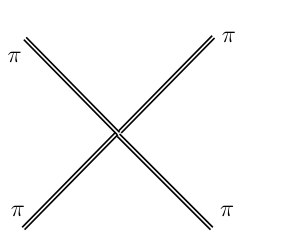
Refer to caption

Figure 3: DMP →\to DMP scattering diagram.

In terms of DMP defined in the Cartan basis

𝝅2=∑iπi2+2​∑𝜶>0π𝜶​π−𝜶;π𝜶†=π−𝜶,{\bm{\pi}}^{2}=\sum_{i}\pi_{i}^{2}+2\sum_{{\bm{\alpha}}>0}\pi_{\bm{\alpha}}\pi_{-{\bm{\alpha}}}\,;\qquad\pi_{\bm{\alpha}}^{\dagger}=\pi_{-{\bm{\alpha}}}\,, (79)

we have the following reactions:

reactionLagrangianamplitudecrosssectioni​i→j​j​(i≠j)−(u/4)​πi2​(□+μ2)​πj2i​u​(s−μ2)σ0/2i​i→i​i−(u/8)​πi2​(□+μ2)​πi2i​u​(4​M2−3​μ2)u2​(M2−34​μ2)2/(2​π​s)i​i→𝜶​𝜶¯−(u/2)​πi2​(□+μ2)​|π𝜶|2i​u​(s−μ2)σ0𝜶​𝜶¯→i​i−(u/2)​πi2​(□+μ2)​|π𝜶|2i​u​(s−μ2)σ0/2𝜶​𝜶¯→𝜷​𝜷¯​(𝜶≠𝜷)−u​|π𝜷|2​(□+μ2)​|π𝜶|2i​u​(s−μ2)σ0𝜶​𝜶¯→𝜶​𝜶¯−(u/2)​|π𝜶|2​(□+μ2)​|π𝜶|22​i​u​(M2−μ2)u2​(M2−μ2)2/(4​π​s)\begin{array}[]{llll}{\rm reaction}&{\rm\qquad Lagrangian}&{\rm amplitude}&{\rm crosssection}\cr\hline\cr ii\to jj~(i\not=j)&-(u/4)\pi_{i}^{2}(\square+\mu^{2})\pi_{j}^{2}&iu(s-\mu^{2})&\sigma_{0}/2\cr ii\to ii&-(u/8)\pi_{i}^{2}(\square+\mu^{2})\pi_{i}^{2}&iu(4M^{2}-3\mu^{2})&u^{2}\left(M^{2}-\frac{3}{4}\mu^{2}\right)^{2}/(2\pi s)\cr ii\to{\bm{\alpha}}\bar{\bm{\alpha}}&-(u/2)\pi_{i}^{2}(\square+\mu^{2})|\pi_{\bm{\alpha}}|^{2}&iu(s-\mu^{2})&\sigma_{0}\cr{\bm{\alpha}}\bar{\bm{\alpha}}\to ii&-(u/2)\pi_{i}^{2}(\square+\mu^{2})|\pi_{\bm{\alpha}}|^{2}&iu(s-\mu^{2})&\sigma_{0}/2\cr{\bm{\alpha}}\bar{\bm{\alpha}}\to{\bm{\beta}}\bar{\bm{\beta}}~({\bm{\alpha}}\not={\bm{\beta}})&-u|\pi_{\bm{\beta}}|^{2}(\square+\mu^{2})|\pi_{\bm{\alpha}}|^{2}&iu(s-\mu^{2})&\sigma_{0}\cr{\bm{\alpha}}\bar{\bm{\alpha}}\to{\bm{\alpha}}\bar{\bm{\alpha}}&-(u/2)|\pi_{\bm{\alpha}}|^{2}(\square+\mu^{2})|\pi_{\bm{\alpha}}|^{2}&2iu(M^{2}-\mu^{2})&u^{2}\left(M^{2}-\mu^{2}\right)^{2}/(4\pi s)\end{array} (80)

where 𝜶¯=−𝜶,𝜷¯=−𝜷\bar{\bm{\alpha}}=-{\bm{\alpha}},~\bar{\bm{\beta}}=-{\bm{\beta}}, and

σ0=u2​(s−μ2)216​π​s,u=N2​f2​(N2−2).\sigma_{0}=\frac{u^{2}(s-\mu^{2})^{2}}{16\pi s}\,,\qquad u=\frac{N}{2f^{2}(N^{2}-2)}\,. (81)

3.4 Decays of SM particles to DMP

Limits on the DMP parameters can be derived either from collider reactions or from potential deviations from SM decays. Reactions of the form f​f¯→π​πf\bar{f}\to\pi\pi, where ff is a SM fermion, or WW fusion reactions W​W→π​πWW\to\pi\pi, would mimic neutrino production at colliders. The limits, however, are very weak since these processes proceed through a virtual hh and so the amplitude will be proportional to small Yukawa coupling, or, for the case of heavy initial quarks, suppressed distribution functions.

The main limits are then derived form the two leading decay processes, Fig.4, namely, h→π​πh\to\pi\pi and Z→π​π​πZ\to\pi\pi\pi, to which we now turn.

Refer to caption     Refer to caption

Figure 4: SM particle decays to DMP.

h→𝝅​𝝅h\to{\bm{\pi}}{\bm{\pi}} decay

Using () and choosing a Hermitian π\pi basis we find that the width is given by

Γ⁡(h→πa​πb)=Γh​π​π​δa​b;Γh​π​π=(λh​v)216​π​mh​(mh2−2​M22​f2)2​1−4​M2mh2​θ​(mh−2​M);\Gamma(h\to\pi_{a}\pi_{b})=\Gamma_{h\pi\pi}\delta_{ab}\,;\quad\Gamma_{h\pi\pi}=\frac{(\lambda_{h}v)^{2}}{16\pi m_{h}}\left(\frac{m_{h}^{2}-2M^{2}}{2f^{2}}\right)^{2}\sqrt{1-\frac{4M^{2}}{m_{h}^{2}}}\,\theta(m_{h}-2M)\,; (82)

in the Cartan basis Γ⁡(h→πi​πi)=Γh​π​π\Gamma(h\to\pi_{i}\pi_{i})=\Gamma_{h\pi\pi} and Γ⁡(h→π𝜶​π−𝜶)=2​Γh​π​π\Gamma(h\to\pi_{\bm{\alpha}}\pi_{-{\bm{\alpha}}})=2\Gamma_{h\pi\pi}. Recent data [35] favors a Higgs decay close to the SM prediction of ∼4​MeV\sim 4\,\hbox{MeV} and a mass mh∼125​GeVm_{h}\sim 125\,\hbox{GeV}; this requires M>mh/2M>m_{h}/2, or M<mh/2M<m_{h}/2 and Γh​π​π<4​MeV\Gamma_{h\pi\pi}<4\,\hbox{MeV}, hence the constraint we use is

f>5.9​|λh|1/2​|7812.5−M2|1/2​[1−(M62.5)2]1/8,M<62.5​(M​in​GeV).f>5.9|\lambda_{h}|^{1/2}|7812.5-M^{2}|^{1/2}\left[1-\left(\frac{M}{62.5}\right)^{2}\right]^{1/8}\,,\qquad M<62.5~(M~\hbox{in}~\hbox{GeV})\,. (83)

In the numerical solutions to Boltzmann equations for DMP for the S​U​(2){SU(2)} case (discussed below), we consider DMP masses in the interval 50​GeV≤M≤2000​GeV50\,\hbox{GeV}\leq M\leq 2000\,\hbox{GeV} so the h→𝝅​𝝅h\to{\bm{\pi}}{\bm{\pi}} constraint plays an important role only for comparatively small values of MM.

Z→𝝅​𝝅​𝝅Z\to{\bm{\pi}}{\bm{\pi}}{\bm{\pi}} decay

The calculation is straightforward; using again a Hermitian DMP basis we find

Γ⁡(Z→π​π​π)=M7​sw2​λV215​(8​π​f2)3​r5/2​(∑a>b>c|fa​b​c|2)​[pE​𝐄​(c)+pK​𝐊​(c)],\Gamma(Z\to\pi\pi\pi)=\frac{M^{7}s_{\rm w}^{2}\lambda_{V}^{2}}{15\,(8\pi f^{2})^{3}\,r^{5/2}}\left(\sum_{a>b>c}|f_{abc}|^{2}\right)\left[p_{E}{\bf E}(c)+p_{K}{\bf K}(c)\right]\,, (84)

where sw=sin⁡θws_{\rm w}=\sin\theta_{\rm w}, while 𝐄,𝐊{\bf E},\,{\bf K} denote the usual Elliptic functions, and

pE\displaystyle p_{E} =\displaystyle= (3​r8+394​r6−720​r4+54​r2−243),\displaystyle(3r^{8}+394r^{6}-720r^{4}+54r^{2}-243)\,, (85)
pK\displaystyle p_{K} =\displaystyle= −12​(r−1)3​(20​r6+63​r5+99​r4+522​r3+918​r2+567​r+243),\displaystyle-\frac{1}{2}(r-1)^{3}(20r^{6}+63r^{5}+99r^{4}+522r^{3}+918r^{2}+567r+243)\,, (86)
c\displaystyle c =\displaystyle= −(r−3)​(1+r)316​r,\displaystyle-\frac{(r-3)(1+r)^{3}}{16r}\,, (87)
r\displaystyle r =\displaystyle= mZM.\displaystyle\frac{m_{Z}}{M}\,. (88)

For ℋDM=S​U​(N){\cal H}_{\rm DM}={SU(N)} and our normalization conventions (13,14) the summation involving the structure constants is given by

∑a>b>c|fa​b​c|2=13!​∑a,b,c|fa​b​c|2=N⁡(N2−1)3.\sum_{a>b>c}|f_{abc}|^{2}=\frac{1}{3!}\sum_{a,b,c}|f_{abc}|^{2}=\frac{N(N^{2}-1)}{3}\,. (89)

Using the uncertainty in the invisible width of the ZZ, Γ​(Z)inv\Gamma(Z)_{\rm inv} we have limit

Γ⁡(Z→π​π​π)<3×10⁻³​Γ​(Z)inv=3×10⁻³​g2​mZ32​π​cw2,{\Gamma(Z\to\pi\pi\pi)}{}<3\times 10^{-3}\Gamma(Z)_{\rm inv}=3\times 10^{-3}\frac{g^{2}m_{Z}}{32\pi c_{\rm w}^{2}}\,, (90)

which implies

55.4>N⁡(N2−1)​(mZ3​λVf3)2​Q,55.4>N(N^{2}-1)\left(\frac{m_{Z}^{3}\lambda_{V}}{f^{3}}\right)^{2}Q\,, (91)

where

Q=r−19/2[pE𝐄(u)+pK𝐊(u)].Q=r^{-19/2}[p_{E}{\bf E}(u)+p_{K}{\bf K}(u)]\,. (92)

The function QQ is monotonic; it vanishes as r→3r\to 3 and approaches 0.750.75 as r→∞r\to\infty. Taking N=2N=2, and λV=0.63\lambda_{V}=0.63, the most conservative limit (corresponding to taking Q=3/4Q=3/4) corresponds to

f>51.43​GeV(M<mz3).f>51.43\,\hbox{GeV}\quad\left(M<\frac{m_{z}}{3}\right)\,. (93)

When λV=0.063\lambda_{V}=0.063, this limit becomes f>23.87​GeVf>23.87\,\hbox{GeV}.

In the numerical analysis, we choose to work with DMP mass ≥50​GeV\geq 50\,\hbox{GeV} and therefore the constraint from Z→π​π​πZ\to\pi\pi\pi is of no importance.

4 Thermal history of DMP

We now turn to the derivation of the relic abundance of DMP. We follow the standard treatment (see e.g. [39]) and will consider only 2→22\to 2 processes.

4.1 Boltzmann equations

The change in the number density of particle of type aa due to collisions and the expansion of the universe is given by

n˙a+3​H​na\displaystyle\dot{n}_{a}+3Hn_{a} =\displaystyle= −𝒞a,\displaystyle-{\cal C}_{a}\,, (94)
𝒞a\displaystyle{\cal C}_{a} =\displaystyle= ∑b,c,d∫d​Φ​|𝒜a+b→c+d|2​(fa​fb−fc​fd),\displaystyle\sum_{b,c,d}\int d\Phi|{\cal A}_{a+b\to c+d}|^{2}(f_{a}f_{b}-f_{c}f_{d})\,, (95)
d​Φ\displaystyle d\Phi =\displaystyle= d​Πa​d​Πb​d​Πc​d​Πd​(2​π)4​δ(4)​(pa+pb−pc−pd),\displaystyle d\Pi_{a}\,d\Pi_{b}\,d\Pi_{c}\,d\Pi_{d}(2\pi)^{4}\delta^{\left(4\right)}(p_{a}+p_{b}-p_{c}-p_{d})\,, (96)

where d​Πd\Pi denotes the phase-space volume

d​Π=g2​E𝐩​d3​𝐩(2​π)3,d\Pi=\frac{g}{2E_{\bf p}}\frac{d^{3}{\bf p}}{(2\pi)^{3}}\,, (97)

and gg is the number of internal degrees of freedom. The amplitude-squared |𝒜|2|{\cal A}|^{2} for the a+b→c+da+b\to c+d process is understood to be averaged over initial and final states, and to include symmetry factors for identical particles in the final states. The functions ff are the particle phase-space distribution functions; the corresponding particle number density is

n=g​∫d3​𝐩(2​π)3​f.n=g\int\frac{d^{3}{\bf p}}{(2\pi)^{3}}f\,. (98)

We will assume that interactions are such that kinetic equilibrium is maintained [40]; we will also assume that particles densities are sufficiently small to ignore the effects of quantum statistics. In this case the energy dependence in the distribution functions is given by the Boltzmann factor: f=ζexp(−E/T)f=\zeta\exp(-E/T). Since we are interested in the epoch when the DMP first decouple, all distribution functions will have the same temperature TT; this will continue after decoupling provided no mass thresholds are crossed, or phase transitions occur.

The equilibrium distributions for a particle of mass mm is given by

n(eq)\displaystyle n^{\left({\rm eq}\right)} =\displaystyle= gz∫d3​𝐩(2​π)3e−E/T=z​g​m32​π2K2​(x)x,E=m2+𝐩2,x=mT\displaystyle gz\int\frac{d^{3}{\bf p}}{(2\pi)^{3}}e^{-E/T}=\frac{zgm^{3}}{2\pi^{2}}\frac{K_{2}(x)}{x}\,,\quad E=\sqrt{m^{2}+{\bf p}^{2}}\,,~x=\frac{m}{T} (99)

where zz is the fugacity in equilibrium. For the SM zSM=1z_{\rm SM}=1 to very good accuracy [41]; for the DMP, however, we will allow non-zero chemical potentials. Using the definition in (40) and the discussion below it, it follows that

μj(i)=0,μ𝜶(i)=−μ−𝜶(i),\mu^{\left(i\right)}_{j}=0\,,\qquad\mu^{\left(i\right)}_{\bm{\alpha}}=-\mu^{\left(i\right)}_{-{\bm{\alpha}}}\,, (100)

where μa(i)\mu_{a}^{\left(i\right)} denotes the chemical potential for particle aa associated with charge QiQ_{i} so that z≠1z\not=1 for those particles with non-zero conserved charges, as defined in Sec. 2.1.

Substituting these definitions in the expression for 𝒞{\cal C} and using the standard definition of the scattering cross section σ\sigma we find

𝒞a\displaystyle{\cal C}_{a} =\displaystyle= ∑b,c,d(n~a​n~b−na(eq)​nb(eq)nc(eq)​nd(eq)​n~c​n~d)​⟨σ​v⟩a+b→c+d,\displaystyle\sum_{b,c,d}\left(\tilde{n}_{a}\tilde{n}_{b}-\frac{n^{\left({\rm eq}\right)}_{a}n^{\left({\rm eq}\right)}_{b}}{n^{\left({\rm eq}\right)}_{c}n^{\left({\rm eq}\right)}_{d}}\tilde{n}_{c}\tilde{n}_{d}\right)\left\langle\sigma v\right\rangle_{a+b\to c+d}\,, (101)
⟨σ​v⟩a+b→c+d\displaystyle\left\langle\sigma v\right\rangle_{a+b\to c+d} =\displaystyle= T​ga​gb2​(2​π)4​na(eq)​nb(eq)​∫so∞d​s​λ⁡(s,mb2,ma2)s​K1​(s/T)​σa+b→c+d​(s),\displaystyle\frac{Tg_{a}g_{b}}{2\,(2\pi)^{4}n^{\left({\rm eq}\right)}_{a}n^{\left({\rm eq}\right)}_{b}}\int_{s_{o}}^{\infty}ds\,\frac{\lambda(s,m_{b}^{2},m_{a}^{2})}{\sqrt{s}}K_{1}(\sqrt{s}/T)\,\sigma_{a+b\to c+d}(s)\,, (103)

where n~=z​n\tilde{n}=zn, s=(pa+pb)2=ma2+mb2+2​pa.pbs=(p_{a}+p_{b})^{2}=m_{a}^{2}+m_{b}^{2}+2p_{a}.p_{b}, λ⁡(a,b,c)\lambda(a,b,c) is defined in (71), and

so=max⁡{(ma+mb)2,(mc+md)2}.s_{o}={\rm max}\{(m_{a}+m_{b})^{2},(m_{c}+m_{d})^{2}\}\,. (104)

In the definition of sos_{o} we used the condition (contained in the cross section) that ss should be large enough to create cc and dd.

For the pure DMP scattering processes that appear in the Boltzmann equations the averaged cross sections can be evaluated in closed form. We obtain, for example

⟨σ​v⟩πi​πi→π𝜶​π−𝜶\displaystyle\left\langle\sigma v\right\rangle_{\pi_{i}\pi_{i}\to\pi_{\bm{\alpha}}\pi_{-{\bm{\alpha}}}} =\displaystyle= 18​xzπa​zπb​[K2​(x)]2​1M5​∫4​M2∞d​s​s​(s−4​M2)​K1​(s/T)​σ0\displaystyle\frac{1}{8}\frac{x}{z_{\pi_{a}}z_{\pi_{b}}[K_{2}(x)]^{2}}\frac{1}{M^{5}}\int_{4M^{2}}^{\infty}ds\,\sqrt{s}\,(s-4M^{2})K_{1}(\sqrt{s}/T)\,\sigma_{0} (105)
=\displaystyle= 4​u2​M2π​1zπa​zπb​x3​[K2​(x)]2​[B​x2+3x​K2​(2​x)+B2​x2+64​K1​(2​x)],\displaystyle\frac{4u^{2}M^{2}}{\pi}\frac{1}{z_{\pi_{a}}z_{\pi_{b}}x^{3}[K_{2}(x)]^{2}}\left[\frac{Bx^{2}+3}{x}K_{2}(2x)+\frac{B^{2}x^{2}+6}{4}K_{1}(2x)\right]\,, (106)

with similar expressions for the other relevant processes; in deriving this we used (80) and (81). For the relevant initial states (πi​πi\pi_{i}\pi_{i} or π𝜶​π−𝜶\pi_{\bm{\alpha}}\pi_{-{\bm{\alpha}}}) we have zi=1=z𝜶​z−𝜶z_{i}=1=z_{{\bm{\alpha}}}z_{-{\bm{\alpha}}} so that in all cases of interest (see below) we can replace zπa​zπb→1z_{\pi_{a}}z_{\pi_{b}}\to 1. Also uu is defined in (81), while BB is defined as

B=1−μ24​M2=N4−12​N2+1N2​(N2+1)B=1-\frac{\mu^{2}}{4M^{2}}=\frac{N^{4}-\frac{1}{2}N^{2}+1}{N^{2}(N^{2}+1)} (107)

and μ\mu is given in (77). In deriving the above result we used

∫1∞d​y​(y2−1)n​K1​(2​x​y)=n!2​Kn​(2​x)xn+1.\int_{1}^{\infty}dy(y^{2}-1)^{n}K_{1}(2xy)=\frac{n!}{2}\frac{K_{n}(2x)}{x^{n+1}}\,. (108)

With the above preliminaries we can now find the relevant collision terms 𝒞a{\cal C}_{a} (c.f Eq.(96)) for the cases a=πia=\pi_{i} and a=π𝜶a=\pi_{\bm{\alpha}} that we abbreviate as 𝒞i{\cal C}_{i} and 𝒞𝜶{\cal C}_{{}_{\bm{\alpha}}} respectively. We will assume that all SM particles remain in equilibrium, so that nSM=nSM(eq)n_{\rm SM}=n^{\left({\rm eq}\right)}_{\rm SM}. The tables of the relevant reactions (which do not cancel in 𝒞i,α{\cal C}_{i,\alpha} ) are

a=π𝜶bc/dπ−𝜶W+​W−,Z​Z,f​f¯,h​h,πj​V,πj​πj,π𝜷​π−𝜷Vπj​π𝜶,π𝜷​π𝜶−𝜷πjV​π𝜶π𝜷V​π𝜶+𝜷\displaystyle\begin{array}[]{|c|c|}\hline\cr\vrule\lx@intercol\hfil a=\pi_{\bm{\alpha}}\hfil\lx@intercol\vrule\lx@intercol\cr\hline\cr\hline\cr b&c/d\cr\hline\cr\pi_{-{\bm{\alpha}}}&W^{+}W^{-},\;ZZ,\;f\bar{f},\;hh,\;\pi_{j}V,\;\pi_{j}\pi_{j},\;\pi_{\bm{\beta}}\pi_{-{\bm{\beta}}}\cr\hline\cr V&\pi_{j}\pi_{\bm{\alpha}},\;\pi_{\bm{\beta}}\pi_{{\bm{\alpha}}-{\bm{\beta}}}\cr\hline\cr\pi_{j}&V\pi_{\bm{\alpha}}\cr\hline\cr\pi_{\bm{\beta}}&V\pi_{{\bm{\alpha}}+{\bm{\beta}}}\cr\hline\cr\end{array}
(116)
a=πibc/dπiW+​W−,Z​Z,f​f¯,h​h,πj​πj,π𝜷​π−𝜷π𝜷V​π𝜷\displaystyle\begin{array}[]{|c|c|}\hline\cr\vrule\lx@intercol\hfil a=\pi_{i}\hfil\lx@intercol\vrule\lx@intercol\cr\hline\cr\hline\cr b&c/d\cr\hline\cr\pi_{i}&W^{+}W^{-},\;ZZ,\;f\bar{f},\;hh,\;\pi_{j}\pi_{j},\;\pi_{\bm{\beta}}\pi_{-{\bm{\beta}}}\cr\hline\cr\pi_{\bm{\beta}}&V\pi_{\bm{\beta}}\cr\hline\cr\end{array}

where VV represents ZZ or γ\gamma, 𝜷≠−𝜶{\bm{\beta}}\not=-{\bm{\alpha}}, and a summation over jj and 𝜷{\bm{\beta}} is assumed.

Now, using (103) and noting that (100) implies

n~i=ni,n~𝜶​n~−𝜶=n𝜶​n−𝜶,\tilde{n}_{i}=n_{i}\,,\qquad\tilde{n}_{\bm{\alpha}}\tilde{n}_{-{\bm{\alpha}}}=n_{\bm{\alpha}}n_{-{\bm{\alpha}}}\,, (122)

and similarly for the equilibrium densities, we find

𝒞i\displaystyle{\cal C}_{i} =\displaystyle= (ni2−ni(eq))2⟨σv⟩πi​πi→S​M+∑𝜶n~𝜶(ni−ni(eq))[⟨σv⟩πi​π𝜶→γ​π𝜶+⟨σv⟩πi​π𝜶→Z​π𝜶]\displaystyle(n_{i}^{2}-n^{\left({\rm eq}\right)}_{i}{}^{2})\left\langle\sigma v\right\rangle_{\pi_{i}\pi_{i}\to SM}+\sum_{\bm{\alpha}}\tilde{n}_{\bm{\alpha}}\left(n_{i}-n^{\left({\rm eq}\right)}_{i}\right)\left[\left\langle\sigma v\right\rangle_{\pi_{i}\pi_{\bm{\alpha}}\to\gamma\pi_{\bm{\alpha}}}+\left\langle\sigma v\right\rangle_{\pi_{i}\pi_{\bm{\alpha}}\to Z\pi_{\bm{\alpha}}}\right] (125)
+∑𝜶ni(eq)(nini(eq)−n𝜶n𝜶(eq)n−𝜶n−𝜶(eq))[nZ(eq)⟨σv⟩πi​Z→π𝜶​π−𝜶+nγ(eq)⟨σv⟩πi​γ→π𝜶​π−𝜶]\displaystyle\quad+\sum_{\bm{\alpha}}n^{\left({\rm eq}\right)}_{i}\left(\frac{n_{i}}{n^{\left({\rm eq}\right)}_{i}}-\frac{n_{\bm{\alpha}}}{n^{\left({\rm eq}\right)}_{\bm{\alpha}}}\frac{n_{-{\bm{\alpha}}}}{n^{\left({\rm eq}\right)}_{-{\bm{\alpha}}}}\right)\left[n^{\left({\rm eq}\right)}_{Z}\left\langle\sigma v\right\rangle_{\pi_{i}Z\to\pi_{\bm{\alpha}}\pi_{-{\bm{\alpha}}}}+n^{\left({\rm eq}\right)}_{\gamma}\left\langle\sigma v\right\rangle_{\pi_{i}\gamma\to\pi_{\bm{\alpha}}\pi_{-{\bm{\alpha}}}}\right]
+∑j≠i(ni2−n(eq)i2n(eq)j2nj2)⟨σv⟩πi​πi→πj​πj+∑𝜶(ni2−n(eq)i2n𝜶(eq)​n−𝜶(eq)n𝜶n−𝜶)⟨σv⟩πi​πi→π𝜶​π−𝜶\displaystyle\quad+\sum_{j\not=i}\left(n_{i}^{2}-\frac{n^{\left({\rm eq}\right)}_{i}{}^{2}}{n^{\left({\rm eq}\right)}_{j}{}^{2}}n_{j}^{2}\right)\left\langle\sigma v\right\rangle_{\pi_{i}\pi_{i}\to\pi_{j}\pi_{j}}+\sum_{\bm{\alpha}}\left(n_{i}^{2}-\frac{n^{\left({\rm eq}\right)}_{i}{}^{2}}{n^{\left({\rm eq}\right)}_{\bm{\alpha}}n^{\left({\rm eq}\right)}_{-{\bm{\alpha}}}}n_{\bm{\alpha}}n_{-{\bm{\alpha}}}\right)\left\langle\sigma v\right\rangle_{\pi_{i}\pi_{i}\to\pi_{\bm{\alpha}}\pi_{-{\bm{\alpha}}}}

and

𝒞𝜶\displaystyle{\cal C}_{\bm{\alpha}} =\displaystyle= (n𝜶​n−𝜶−n𝜶(eq)​n−𝜶(eq))​⟨σ​v⟩π𝜶​π−𝜶→S​M\displaystyle(n_{\bm{\alpha}}n_{-{\bm{\alpha}}}-n^{\left({\rm eq}\right)}_{\bm{\alpha}}n^{\left({\rm eq}\right)}_{-{\bm{\alpha}}})\left\langle\sigma v\right\rangle_{\pi_{\bm{\alpha}}\pi_{-{\bm{\alpha}}}\to SM} (129)
+∑i(n𝜶n−𝜶−n𝜶(eq)n−𝜶(eq)nini(eq))[⟨σv⟩π𝜶​π−𝜶→πi​γ+⟨σv⟩π𝜶​π−𝜶→πi​Z]\displaystyle\quad+\sum_{i}\left(n_{\bm{\alpha}}n_{-{\bm{\alpha}}}-n^{\left({\rm eq}\right)}_{\bm{\alpha}}n^{\left({\rm eq}\right)}_{-{\bm{\alpha}}}\frac{n_{i}}{n^{\left({\rm eq}\right)}_{i}}\right)\left[\left\langle\sigma v\right\rangle_{\pi_{\bm{\alpha}}\pi_{-{\bm{\alpha}}}\to\pi_{i}\gamma}+\left\langle\sigma v\right\rangle_{\pi_{\bm{\alpha}}\pi_{-{\bm{\alpha}}}\to\pi_{i}Z}\right]
+∑i(n𝜶n−𝜶−n𝜶(eq)​n−𝜶(eq)n(eq)i2ni2)⟨σv⟩π𝜶​π−𝜶→πi​πi\displaystyle\quad+\sum_{i}\left(n_{\bm{\alpha}}n_{-{\bm{\alpha}}}-\frac{n^{\left({\rm eq}\right)}_{\bm{\alpha}}n^{\left({\rm eq}\right)}_{-{\bm{\alpha}}}}{n^{\left({\rm eq}\right)}_{i}{}^{2}}n_{i}^{2}\right)\left\langle\sigma v\right\rangle_{\pi_{\bm{\alpha}}\pi_{-{\bm{\alpha}}}\to\pi_{i}\pi_{i}}
+∑𝜷≠±𝜶(n𝜶n−𝜶−n𝜶(eq)​n−𝜶(eq)n𝜷(eq)​n−𝜷(eq)n𝜷n−𝜷)⟨σv⟩π𝜶​π−𝜶→π𝜷​π−𝜷,\displaystyle\quad+\sum_{{\bm{\beta}}\not=\pm{\bm{\alpha}}}\left(n_{\bm{\alpha}}n_{-{\bm{\alpha}}}-\frac{n^{\left({\rm eq}\right)}_{\bm{\alpha}}n^{\left({\rm eq}\right)}_{-{\bm{\alpha}}}}{n^{\left({\rm eq}\right)}_{\bm{\beta}}n^{\left({\rm eq}\right)}_{-{\bm{\beta}}}}n_{\bm{\beta}}n_{-{\bm{\beta}}}\right)\left\langle\sigma v\right\rangle_{\pi_{\bm{\alpha}}\pi_{-{\bm{\alpha}}}\to\pi_{\bm{\beta}}\pi_{-{\bm{\beta}}}}\,, (130)

where the contributions coming from π𝜶​V→πi​π𝜶\pi_{\bm{\alpha}}V\to\pi_{i}\pi_{\bm{\alpha}} (V=Z,γV=Z,\,\gamma) and π𝜶​πi→V​π𝜶\pi_{\bm{\alpha}}\pi_{i}\to V\pi_{\bm{\alpha}} cancel, as do those from π𝜶​π𝜷→V​π𝜶+𝜷\pi_{\bm{\alpha}}\pi_{\bm{\beta}}\to V\pi_{{\bm{\alpha}}+{\bm{\beta}}} and π𝜶​V→π𝜷​π𝜶−𝜷\pi_{\bm{\alpha}}V\to\pi_{\bm{\beta}}\pi_{{\bm{\alpha}}-{\bm{\beta}}}. We have also defined, using (103),

⟨σ​v⟩πi​πi→S​M\displaystyle\left\langle\sigma v\right\rangle_{\pi_{i}\pi_{i}\to SM} =\displaystyle= ⟨σ​v⟩πi​πi→W​W+⟨σ​v⟩πi​πi→Z​Z+∑f⟨σ​v⟩πi​πi→f​f+⟨σ​v⟩πi​πi→h​h\displaystyle\left\langle\sigma v\right\rangle_{\pi_{i}\pi_{i}\to WW}+\left\langle\sigma v\right\rangle_{\pi_{i}\pi_{i}\to ZZ}+\sum_{f}\left\langle\sigma v\right\rangle_{\pi_{i}\pi_{i}\to ff}+\left\langle\sigma v\right\rangle_{\pi_{i}\pi_{i}\to hh} (131)
=\displaystyle= T32π4n(eq)i2∫0∞dss3/2K1(s/T)β2[σπi​πi→W​W+σπi​πi→Z​Z\displaystyle\frac{T}{32\pi^{4}n^{\left({\rm eq}\right)}_{i}{}^{2}}\int_{0}^{\infty}ds\,s^{3/2}\,K_{1}(\sqrt{s}/T)\beta^{2}\biggl[\sigma_{\pi_{i}\pi_{i}\to WW}+\sigma_{\pi_{i}\pi_{i}\to ZZ} (133)
+∑fσπi​πi→f​f¯+σπi​πi→h​h]\displaystyle\qquad+\sum_{f}\sigma_{\pi_{i}\pi_{i}\to f\bar{f}}+\sigma_{\pi_{i}\pi_{i}\to hh}\biggr]

and similarly for π𝜶​π−𝜶→S​M\pi_{\bm{\alpha}}\pi_{-{\bm{\alpha}}}\to SM.

4.2 Contributions from SM→\toDMP decays

The effects of Higgs decays into DMP, when kinematically allowed, can be included in the Boltzmann equation in two equivalent ways. We can include them in the total hh width:

Γh=ΓhSM+Γ⁡(h→π​π)\Gamma_{h}=\Gamma_{h}^{\rm SM}+\Gamma(h\to\pi\pi) (134)

and use this expression in the cross sections involving Higgs exchange. Or, alternatively, we can exclude these effects from the Higgs propagators (see e.g. [42]) :

mh​Γh(s−mh2)2+mh2​Γh2\displaystyle\frac{m_{h}\Gamma_{h}}{(s-m_{h}^{2})^{2}+m_{h}^{2}\Gamma_{h}^{2}} →\displaystyle\to mh​Γh(s−mh2)2+mh2​Γh2−π​δ​(s−mh2)​Θ​(s−4​mi2).\displaystyle\frac{m_{h}\Gamma_{h}}{(s-m_{h}^{2})^{2}+m_{h}^{2}\Gamma_{h}^{2}}-\pi\delta(s-m_{h}^{2})\Theta(s-4m_{i}^{2})\,. (135)

and include them in suitable additions 𝒞i,α(decay){\cal C}_{i,\alpha}^{\left(\rm decay\right)} to the collision terms; explicitly (see Appendix A)

𝒞i(decay)\displaystyle{\cal C}_{i}^{\left(\rm decay\right)} =\displaystyle= NHi​nH(eq)​K1​(xH)K2​(xH)​Γ​(h→π​π)\displaystyle N_{H}^{i}n^{\left({\rm eq}\right)}_{H}\frac{K_{1}(x_{H})}{K_{2}(x_{H})}\Gamma(h\to\pi\pi) (136)

where Nh(i)N_{h}^{\left(i\right)} counts the number of produced πi\pi_{i}: Nh(i)=2!N_{h}^{\left(i\right)}=2! for h→πi​πih\to\pi_{i}\pi_{i} and Nh(i)=1N_{h}^{\left(i\right)}=1 for h→π𝜶​π−𝜶h\to\pi_{\bm{\alpha}}\pi_{-{\bm{\alpha}}}; Γ⁡(h→π​π)\Gamma(h\to\pi\pi) is given in (82), and xi=mi/Tx_{i}=m_{i}/T. An analogous equation holds for 𝒞𝜶(decay){\cal C}_{\bm{\alpha}}^{\left(\rm decay\right)}.

If we assume that the recently observed particle at the LHC [35] is the SM Higgs, it’s very small total width ensures that the effects from Higgs decay to DMP are negligible. We have checked that for realistic DMP masses the contribution of Z→π​π​πZ\to\pi\pi\pi decays in the Boltzmann equations (see Appendix A) are also negligible.

5 Solving the Boltzmann equations for the S​U​(2){SU(2)} case

The simplest non-trivial group is ℋDM=S​U​(2){\cal H}_{\rm DM}={SU(2)}, which we consider as an illustrative example of the formalism; the same approach can be used for any NN, though with the calculations become increasingly cumbersome. For N=2N=2 there is a single conserved charge and 3 DMP states that we label as o,±o,\pm, with the first associated with the Cartan generator.

As usually we find it convenient to rewrite the Boltzmann equations (BE) (96, , 130) by defining

x=MT,Yr=1s​nr,Yr(eq)=1s​nr(eq),x=\frac{M}{T}\,,\qquad Y_{r}=\frac{1}{s}n_{r}\,,\qquad Y^{{\rm(eq)}}_{r}=\frac{1}{s}n^{\left({\rm eq}\right)}_{r}\,, (137)

where TT denotes the photon temperature and ss the entropy density:

s=2​π245​gs​(T)​T3;gs​(T)=∑krk​gk​(TkT)3​θ​(T−mk);s=\frac{2\pi^{2}}{45}g_{s}(T)T^{3}\,;\quad g_{s}(T)=\sum_{k}r_{k}g_{k}\left(\frac{T_{k}}{T}\right)^{3}\theta(T-m_{k})\,; (138)

here kk runs over all particles, TkT_{k} is the temperature of particle kk and gkg_{k} its number of internal degrees of freedom, and rk=1​(7/8)r_{k}=1\,(7/8) when kk is a bosons (fermion). We will also make use of Friedman’s equation,

H2=8​π​G3​ρ=4​π3​G45​g​(T)​T4;g⁡(T)=∑krk​gk​(TkT)4​θ​(T−mk).H^{2}=\frac{8\pi G}{3}\rho=\frac{4\pi^{3}G}{45}g(T)\,T^{4}\,;\quad g(T)=\sum_{k}r_{k}g_{k}\left(\frac{T_{k}}{T}\right)^{4}\theta(T-m_{k})\,. (139)

In the following we will take TkT_{k} for all SM particles (assuming TT is above that of the e+​e−e^{+}e^{-} annihilation epoch), so that gs​(T)=g​(T)g_{s}(T)=g(T); we use the expression for g⁡(T)g(T) in Ref. [43]. The explicit form of the equilibrium distribution is

Yr(eq)=454​π4​grgs​(T)​zr​xr2​K2​(xr)⟶xr≫1ar​zr​xr3/2​e−xr;xr=mrT,ar=454​π4​π2​grgs​(T)Y^{{\rm(eq)}}_{r}=\frac{45}{4\pi^{4}}\frac{g_{r}}{g_{s}(T)}z_{r}x_{r}^{2}K_{2}(x_{r})\stackrel{{\scriptstyle x_{r}\gg 1}}{{\longrightarrow}}a_{r}z_{r}x_{r}^{3/2}e^{-x_{r}}\,;\qquad x_{r}=\frac{m_{r}}{T}\,,~~a_{r}=\frac{45}{4\pi^{4}}\sqrt{\frac{\pi}{2}}\frac{g_{r}}{g_{s}(T)} (140)

where zrz_{r} is the fugacity for particle rr and grg_{r} the number of internal degrees of freedom.

We will also consider model parameters where the SM and DM sectors are in equilibrium for temperatures T>TfT>T_{f}, such that Tf>MT_{f}>M, so that the region of interest is x>1x>1 and the DMP will not contribute55 5 If Tf>MT_{f}>M then the situation is more complicated, the DMP maintain a temperature TπT_{\pi} which is initially TfT_{f}, but then is determined by sπ​(Tπ)​R3=sπ​(Tf)​Rd3s_{\pi}(T_{\pi})R^{3}=s_{\pi}(T_{f})R_{d}^{3} and is in general different form the photon temperature. to the effective number of relativistic degrees of freedom g​(T)=gS​M​(T)g(T)=g_{SM}(T).

In terms of YY the Boltzmann equations take the form

d​Yrd​x=−π​g​(T)45​GMx2Cr(Y),Cr(Y)=1s2𝒞r,(r=o,±)\displaystyle\frac{d\,Y_{r}}{d\,x}=-\sqrt{\frac{\pi g(T)}{45G}}\frac{M}{x^{2}}C_{r}(Y)\;,\qquad C_{r}(Y)=\frac{1}{s^{2}}{\cal C}_{r}\,,\qquad(r=o,\pm) (141)

where the collision terms are

Co​(Y)\displaystyle C_{o}(Y) =\displaystyle= (Yo2−Yo(eq)2)​⟨σ​v⟩πo​πo→S​M+(Yo2−Y+​Y−)​⟨σ​v⟩πo​πo→π+​π−\displaystyle\left({Y_{o}^{2}}-{Y^{{\rm(eq)}}_{o}}^{2}\right)\left\langle\sigma v\right\rangle_{\pi_{o}\pi_{o}\to SM}+\left(Y_{o}^{2}-Y_{+}Y_{-}\right)\left\langle\sigma v\right\rangle_{\pi_{o}\pi_{o}\to\pi_{+}\pi_{-}} (143)
+[Yo​Yo(eq)−Y+​Y−+(Y++Y−)​(Yo−Yo(eq))]​⟨σ​v⟩π+​π−→πo​V,\displaystyle~+\left[Y_{o}Y^{{\rm(eq)}}_{o}-Y_{+}Y_{-}+(Y_{+}+Y_{-})(Y_{o}-Y^{{\rm(eq)}}_{o})\right]\left\langle\sigma v\right\rangle_{\pi_{+}\pi_{-}\to\pi_{o}V}\,,

and

C±​(Y)\displaystyle C_{\pm}(Y) =\displaystyle= (Y+​Y−−Yo(eq)2)​⟨σ​v⟩πo​πo→S​M+(Y+​Y−−Yo2)​⟨σ​v⟩π+​π−→πo​πo\displaystyle\left({Y_{+}Y_{-}}-{Y^{{\rm(eq)}}_{o}}^{2}\right)\left\langle\sigma v\right\rangle_{\pi_{o}\pi_{o}\to SM}+\left(Y_{+}Y_{-}-Y_{o}^{2}\right)\left\langle\sigma v\right\rangle_{\pi_{+}\pi_{-}\to\pi_{o}\pi_{o}} (145)
+(Y+​Y−−Yo​Yo(eq))​⟨σ​v⟩π+​π−→πo​V,\displaystyle~+\left({Y_{+}Y_{-}}-{Y_{o}Y^{{\rm(eq)}}_{o}}\right)\left\langle\sigma v\right\rangle_{\pi_{+}\pi_{-}\to\pi_{o}V}\,,

where we used Y+(eq)​Y−(eq)=Yo(eq)2Y^{{\rm(eq)}}_{+}Y^{{\rm(eq)}}_{-}={Y^{{\rm(eq)}}_{o}}^{2}, and also

Yo(eq)​YZ/γ(eq)​⟨σ​v⟩πo​Z/γ→π+​π−=Yo(eq)​Y±(eq)​⟨σ​v⟩πo​π±→Z/γ​π±=Yo(eq)2​⟨σ​v⟩π+​π−→πo​Z/γ,Y^{{\rm(eq)}}_{o}Y^{{\rm(eq)}}_{Z/\gamma}\left\langle\sigma v\right\rangle_{\pi_{o}Z/\gamma\to\pi_{+}\pi_{-}}=Y^{{\rm(eq)}}_{o}Y^{{\rm(eq)}}_{\pm}\left\langle\sigma v\right\rangle_{\pi_{o}\pi_{\pm}\to Z/\gamma\pi_{\pm}}={Y^{{\rm(eq)}}_{o}}^{2}\left\langle\sigma v\right\rangle_{\pi_{+}\pi_{-}\to\pi_{o}Z/\gamma}\,, (146)

and defined

⟨σ​v⟩π+​π−→πo​V=⟨σ​v⟩π+​π−→πo​γ+⟨σ​v⟩π+​π−→πo​Z.\left\langle\sigma v\right\rangle_{\pi_{+}\pi_{-}\to\pi_{o}V}=\left\langle\sigma v\right\rangle_{\pi_{+}\pi_{-}\to\pi_{o}\gamma}+\left\langle\sigma v\right\rangle_{\pi_{+}\pi_{-}\to\pi_{o}Z}\,. (147)

For the S​U​(2){SU(2)} case there is a single non-trivial chemical potential (100) and an associated conserved charge

q=Y−−Y+.q=Y_{-}-Y_{+}\,. (148)

Using qq, the two independent Boltzmann equations become

d​Y+d​x\displaystyle\frac{dY_{+}}{dx} =\displaystyle= −π​g​(T)45​GMx2{[Y+(Y++q)−Yo(eq)]2⟨σv⟩πo​πo→S​M+[Y+(Y++q)−Yo2]⟨σv⟩π+​π−→πo​πo\displaystyle-\sqrt{\frac{\pi g(T)}{45G}}\frac{M}{x^{2}}\Biggl\{\left[Y_{+}(Y_{+}+q)-Y^{{\rm(eq)}}_{o}{}^{2}\right]\left\langle\sigma v\right\rangle_{\pi_{o}\pi_{o}\to SM}+\left[Y_{+}(Y_{+}+q)-Y_{o}^{2}\right]\left\langle\sigma v\right\rangle_{\pi_{+}\pi_{-}\to\pi_{o}\pi_{o}} (150)
+[Y+(Y++q)−YoYo(eq)]⟨σv⟩π+​π−→πo​V]},\displaystyle\qquad\qquad\qquad\qquad+\left[Y_{+}(Y_{+}+q)-Y_{o}Y^{{\rm(eq)}}_{o}\right]\left\langle\sigma v\right\rangle_{\pi_{+}\pi_{-}\to\pi_{o}V}]\Biggr\}\,,
d​Yod​x\displaystyle\frac{dY_{o}}{dx} =\displaystyle= −π​g​(T)45​GMx2{(Yo2−Yo(eq)2)⟨σv⟩πo​πo→S​M+[Yo2−Y+(Y++q)]⟨σv⟩πo​πo→π+​π−\displaystyle-\sqrt{\frac{\pi g(T)}{45G}}\frac{M}{x^{2}}\Biggl\{\left({Y_{o}^{2}}-{Y^{{\rm(eq)}}_{o}}^{2}\right)\left\langle\sigma v\right\rangle_{\pi_{o}\pi_{o}\to SM}+\left[Y_{o}^{2}-Y_{+}(Y_{+}+q)\right]\left\langle\sigma v\right\rangle_{\pi_{o}\pi_{o}\to\pi_{+}\pi_{-}} (152)
+[(2Y++q)(Yo−Yo(eq))−Y+(Y++q)+YoYo(eq)]⟨σv⟩π+​π−→πo​V}.\displaystyle~+\left[(2Y_{+}+q)(Y_{o}-Y^{{\rm(eq)}}_{o})-Y_{+}(Y_{+}+q)+Y_{o}Y^{{\rm(eq)}}_{o}\right]\left\langle\sigma v\right\rangle_{\pi_{+}\pi_{-}\to\pi_{o}V}\Biggr\}\,. (153)

From (103) we find that

Yo(eq)​YZ/γ(eq)​⟨σ​v⟩πo​Z/γ→π+​π−\displaystyle Y^{{\rm(eq)}}_{o}Y^{{\rm(eq)}}_{Z/\gamma}\left\langle\sigma v\right\rangle_{\pi_{o}{Z/\gamma}\to\pi_{+}\pi_{-}} =\displaystyle= T2​[2​π2​s​(T)]2​∫so∞d​s​P​KV​s​K1​(s/T)​σZ/γ,\displaystyle\frac{T}{2[2\pi^{2}s(T)]^{2}}\int_{s_{o}}^{\infty}ds\,PK_{V}\sqrt{s}K_{1}(\sqrt{s}/T)\sigma^{Z/\gamma}\,, (154)
Yo(eq)⟨σv⟩πo​πo→S​M2\displaystyle Y^{{\rm(eq)}}_{o}{}^{2}\left\langle\sigma v\right\rangle_{\pi_{o}\pi_{o}\to SM} =\displaystyle= T2​[2​π2​s​(T)]2​∫so∞d​s​s​P2​K1​(s/T)​σπo​πo→S​M,\displaystyle\frac{T}{2[2\pi^{2}s(T)]^{2}}\int_{s_{o}}^{\infty}ds\,\sqrt{s}P^{2}K_{1}(\sqrt{s}/T)\sigma_{\pi_{o}\pi_{o}\to SM}\,, (156)

where σZ/γ\sigma^{Z/\gamma} are given in (69) and P,KVP,\,K_{V} are defined in (70).

The ⟨σ​v⟩\left\langle\sigma v\right\rangle are plotted in Fig.5 for a representative parameter space point. The SM cross section is almost xx-independent (corresponding to a predominance of ss-wave scattering), while the γ/Z\gamma/Z cross section is proportional to 1/x1/x, indicating a predominance of pp-wave scattering. It is interesting to note that the DMP→\toDMP cross section has an unusual 1/x1/\sqrt{x} behavior for large xx that results from all particles having the same mass and the amplitude being non-zero and finite at threshold, which for this model is a consequence of the chiral couplings of the DMPs. One can see, that ⟨σ​v⟩π​π→S​M\left\langle\sigma v\right\rangle_{\pi\pi\to SM} is much smaller than ⟨σ​v⟩π​π→π​V\left\langle\sigma v\right\rangle_{\pi\pi\to\pi V} or ⟨σ​v⟩π​π→π​π\left\langle\sigma v\right\rangle_{\pi\pi\to\pi\pi} for the particular choice of parameters. The relevance of ⟨σ​v⟩π​π→S​M\left\langle\sigma v\right\rangle_{\pi\pi\to SM} can be understood by referring to Fig.6 where we compare ⟨σ​v⟩π​π→S​M\left\langle\sigma v\right\rangle_{\pi\pi\to SM} and ⟨σ​v⟩π​π→π​V\left\langle\sigma v\right\rangle_{\pi\pi\to\pi V} at the decoupling temperature (the point at which the DMP particle density begins to deviate significantly from its equilibrium value – see Sec.5.1) for points that satisfy the cold-dark matter (CDM) relic-abundance constraint (see Eq.(183) below).

Figure 5: Cross sections for a representative set of parameters, (M,f,λh,λV)=(1000​GeV, 950​GeV, 0.01, 0.63)(M,f,\lambda_{h},\lambda_{V})=(1000\,\hbox{GeV},\,950\,\hbox{GeV},\,0.01,\,0.63), for which the model satisfies the cold-dark matter and direct-detection constraints. Top curve: 107​x​⟨σ​v⟩π​π→π​V10^{7}x\left\langle\sigma v\right\rangle_{\pi\pi\to\pi V}; middle curve: 1012​⟨σ​v⟩π​π→S​M10^{12}\left\langle\sigma v\right\rangle_{\pi\pi\to SM}; bottom curve: 108​x​⟨σ​v⟩π​π→π​π10^{8}\sqrt{x}\left\langle\sigma v\right\rangle_{\pi\pi\to\pi\pi}. The prefactors are chosen to fit the curves into the same graph and to illustrate the leading xx behavior. All the cross sections are in GeV−2\hbox{GeV}^{-2}.
Refer to caption
Figure 6: Region in the M−fM-f plane allowed by the CMD constraint (183) when q=0q=0, λV=0.63\lambda_{V}=0.63, and |λh|<1|\lambda_{h}|<1. Blue points: subregion where ⟨σ​v⟩π​π→S​M​(x=xf)>⟨σ​v⟩π​π→π​V​(x=xf)\left\langle\sigma v\right\rangle_{\pi\pi\to SM}(x=x_{f})>\left\langle\sigma v\right\rangle_{\pi\pi\to\pi V}(x=x_{f}). Green points: subregion where ⟨σ​v⟩π​π→S​M​(x=xf)<⟨σ​v⟩π​π→π​V​(x=xf)\left\langle\sigma v\right\rangle_{\pi\pi\to SM}(x=x_{f})<\left\langle\sigma v\right\rangle_{\pi\pi\to\pi V}(x=x_{f}). Red points: subregion excluded by the Higgs decay constraint (83).

To obtain the particle densities and their freeze out temperatures it is necessary to solve a system of coupled linear differential equations for {Yo,Y+}\{Y_{o},Y_{+}\} given by (153). The boundary conditions are determined by requiring that at low xx the DM sector is in equilibrium with the SM:

x<xf:Yo=Yo(eq),andY±=Y±(eq)=Y(eq)o2+q24∓q2.x<x_{f}:~~Y_{o}=Y^{{\rm(eq)}}_{o}\,,\quad{\rm and}\quad Y_{\pm}=Y^{{\rm(eq)}}_{\pm}=\sqrt{Y^{{\rm(eq)}}_{o}{}^{2}+\frac{q^{2}}{4}}\mp\frac{q}{2}. (158)

Note that (153) and (158) imply that both the equations and initial conditions are invariant under Y+↔Y−Y_{+}\leftrightarrow Y_{-} and q↔−qq\leftrightarrow-q.

For the following it is useful to note that ⟨σ​v⟩πo​πo→S​M\left\langle\sigma v\right\rangle_{\pi_{o}\pi_{o}\to SM} depends on λh\lambda_{h} only in the combination λh/f2\lambda_{h}/f^{2}, while ⟨σ​v⟩π+​π−→πo​V\left\langle\sigma v\right\rangle_{\pi_{+}\pi_{-}\to\pi_{o}V} depends on λV\lambda_{V} only as λV/f3\lambda_{V}/f^{3}. This implies that we can take M,fM,f and λh\lambda_{h} as independent parameters, fixing λV\lambda_{V} at some convenient value as in (41); any other value of λV\lambda_{V} can be obtained by appropriate rescaling of ff and λh\lambda_{h}.

–

5.1 Zero charge solutions

When q=0q=0 all DMP will have the same initial equilibrium distribution, the relevant solutions to the BE then correspond to Yo,±=YY_{o,\pm}=Y; substituting this (and q=0q=0) in (153) we find

d​Yd​x=−π​g​(T)45​G​Mx2​(Y−Y(eq))​{(Y+Y(eq))​⟨σ​v⟩πo​πo→S​M+Y​⟨σ​v⟩π+​π−→πo​V},\frac{dY}{dx}=-\sqrt{\frac{\pi g(T)}{45G}}\frac{M}{x^{2}}\left(Y-Y^{{\rm(eq)}}\right)\Bigl\{\left(Y+Y^{{\rm(eq)}}\right)\left\langle\sigma v\right\rangle_{\pi_{o}\pi_{o}\to SM}+Y\left\langle\sigma v\right\rangle_{\pi_{+}\pi_{-}\to\pi_{o}V}\Bigr\}\,, (159)

where we drop the o,±o,\pm subindices.

Approximate solutions to this equation are readily obtained. We find that to good accuracy (see Fig.5) the cross sections have an ss and pp wave behaviors for x>10x>10:

⟨σ​v⟩πo​πo→S​M≃σS​M,⟨σ​v⟩π+​π−→πo​V≃1x​σV,\left\langle\sigma v\right\rangle_{\pi_{o}\pi_{o}\to SM}\simeq\sigma_{SM}\,,\qquad\left\langle\sigma v\right\rangle_{\pi_{+}\pi_{-}\to\pi_{o}V}\simeq\frac{1}{x}\sigma_{V}\,, (160)

where σS​M,V\sigma_{SM,V} are approximately xx-independent.

Near the decoupling temperature we write Y=Y(eq)+ΔY=Y^{{\rm(eq)}}+\Delta and neglect terms proportional to d​Δ/d​xd\Delta/dx and Δ2\Delta^{2}; then (159) becomes

Δ≃x22​ϑS​M+ϑV/x;ϑS​M=π​g​(T)45​G​M​σS​M,ϑV=π​g​(T)45​G​M​σV,\Delta\simeq\frac{x^{2}}{2\vartheta_{SM}+\vartheta_{V}/x}\,;\quad\vartheta_{SM}=\sqrt{\frac{\pi g(T)}{45G}}{M\sigma_{SM}}\,,\quad\vartheta_{V}=\sqrt{\frac{\pi g(T)}{45G}}{M\sigma_{V}}\,, (161)

where we also approximated d​Y(eq)/d​x≃−Y(eq)dY^{{\rm(eq)}}/dx\simeq-Y^{{\rm(eq)}}.

For large xx, in contrast, Δ≃Y≫Y(eq)\Delta\simeq Y\gg Y^{{\rm(eq)}} and (159) becomes

d​Δd​x=−ϑS​M​x+ϑVx3​Δ2⇒Δ∞≃xf2ϑS​M​xf+ϑV/2.\frac{d\Delta}{dx}=-\frac{\vartheta_{SM}x+\vartheta_{V}}{x^{3}}\Delta^{2}{\quad\Rightarrow\quad}\Delta_{\infty}\simeq\frac{x_{f}^{2}}{\vartheta_{SM}x_{f}+\vartheta_{V}/2}\,. (162)

where 1/Δ⁡(xf)1/\Delta(x_{f}) is neglected.

Finally the decoupling ‘temperature’ xfx_{f} is obtained from the condition Δ⁡(xf)=c​Y(eq)​(xf)\Delta(x_{f})=cY^{{\rm(eq)}}(x_{f}), where cc is a numerical constant. This gives

Y∞\displaystyle Y_{\infty} =\displaystyle= xf2ϑS​M​xf+ϑV/2,\displaystyle\frac{x_{f}^{2}}{\vartheta_{SM}x_{f}+\vartheta_{V}/2}\,, (163)
xf\displaystyle x_{f} =\displaystyle= ln[ac(c+2)ϑS​Mξ−1/2+ac(c+1)ϑVξ−3/2];ξ=ln[c(ϑS​M+ϑV)a]\displaystyle\ln\left[ac(c+2)\vartheta_{SM}\xi^{-1/2}+ac(c+1)\vartheta_{V}\xi^{-3/2}\right]\,;\quad\xi=\ln[c(\vartheta_{SM}+\vartheta_{V})a] (164)

where aa is defined in (140) and ϑS​M,ϑV\vartheta_{SM},\,\vartheta_{V} in (161); this result is better suited for the case ϑV≫ϑS​M\vartheta_{V}\gg\vartheta_{SM} than the one presented in [39]. We will follow this reference and choose c⁡(c+2)=1c(c+2)=1 or, c≃0.414c\simeq 0.414. In calculating the relic abundance it is important to remember that Y∞Y_{\infty} refers to each DMP species, so that the total abundance will be proportional to 3​Y∞3Y_{\infty}.

An alternative definition of xfx_{f} can be derived by assuming YY is close to Y(eq)Y^{{\rm(eq)}} and casting (159) in the form

xYo(eq)​d​Yd​x=−ΓH​(YYo(eq)−1);ΓH=(2​ϑS​M+ϑVx)​Yo(eq)\frac{x}{Y^{{\rm(eq)}}_{o}}\frac{dY}{dx}=-\frac{\Gamma}{H}\left(\frac{Y}{Y^{{\rm(eq)}}_{o}}-1\right)\,;\qquad\frac{\Gamma}{H}=\left(\frac{2\vartheta_{SM}+\vartheta_{V}}{x}\right)Y^{{\rm(eq)}}_{o} (165)

so xfx_{f} can be defined as the point where Γ/H=1\Gamma/H=1. A plot of Γ/H\Gamma/H for representative values of the parameters, and a comparison with the previous definition of xfx_{f} is given in Fig.7. This also illustrates that xfx_{f} in general is large enough for the approximations (160) to be valid.

In Fig.8 we compare the relic abundance derived numerically with the one obtained from (164), showing that, at least in this instance, the latter is reasonably accurate. From this figure one can also see that the decoupling point inferred from the numerical solutions equals the analytically obtained values within 10%.

Figure 7: Plot of Γ/H\Gamma/H for the same parameters as in Fig.5. We also include the values of xfx_{f} obtained from the condition Δ=c​Y(eq)\Delta=cY^{{\rm(eq)}} for c=0.414, 0.732, 1c=0.414,\,0.732,\,1 (left, center and right heavy dots on the dashed line, respectively). The freeze-out condition Γ=H\Gamma=H corresponds to xf≃31.3x_{f}\simeq 31.3 which coincides almost exactly with the c=1c=1 value.

Figure 8: Plot of the yield YY as a function xx for the representative point of Fig.5 when q=0q=0. Dark matter pion aboundance is depicted in blue, and the equilibrium distribution is shown in red. The heavy dot on the right indicates the value of Y∞Y_{\infty} obtained form (164) using c=1c=1. All masses are in GeV.

5.2 Behavior for small values of |q||q|

We now turn to the case where qq is small but non-vanishing. In this case it is convenient to define

Yt\displaystyle Y_{t} =\displaystyle= Yo+Y++Y−=Yo+2​Y++q,\displaystyle Y_{o}+Y_{+}+Y_{-}=Y_{o}+2Y_{+}+q\,, (166)
Yd\displaystyle Y_{d} =\displaystyle= Y++Y−2−Yo=Y+−Yo+q2,\displaystyle\frac{Y_{+}+Y_{-}}{2}-Y_{o}=Y_{+}-Y_{o}+\frac{q}{2}\,, (167)

in terms of which Eqs.(153) become

Yt′\displaystyle Y_{t}^{\prime} =\displaystyle= −13​(yt2+2​yd2)​(A+B)+(yt+yd2)​B+[q24​(2​A+B)+3​A],\displaystyle-\frac{1}{3}(y_{t}^{2}+2y_{d}^{2})(A+B)+(y_{t}+y_{d}^{2})B+\Biggl[\frac{q^{2}}{4}(2A+B)+3A\Biggr]\,, (168)
Yd′\displaystyle Y_{d}^{\prime} =\displaystyle= 13​yd​(yd−2​yt)​(A+B+32​C)−yd​(yd+2)​B+q24​(A+3​B+32​C),\displaystyle\frac{1}{3}y_{d}(y_{d}-2y_{t})\left(A+B+\frac{3}{2}C\right)-y_{d}(y_{d}+2)B+\frac{q^{2}}{4}\left(A+3B+\frac{3}{2}C\right)\,, (169)

where yt,d=Yt,d/Yo(eq)y_{t,d}=Y_{t,d}/Y^{{\rm(eq)}}_{o} and

{A,B,C}=π​g​(T)45​GMx2Yo(eq){⟨σv⟩πo​πo→S​M,⟨σv⟩π+​π−→πo​V,⟨σv⟩πo​πo→π+​π−}2,\{A,\,B,\,C\}=\sqrt{\frac{\pi g(T)}{45G}}\frac{M}{x^{2}}Y^{{\rm(eq)}}_{o}{}^{2}\{\left\langle\sigma v\right\rangle_{\pi_{o}\pi_{o}\to SM},\;\left\langle\sigma v\right\rangle_{\pi_{+}\pi_{-}\to\pi_{o}V},\;\left\langle\sigma v\right\rangle_{\pi_{o}\pi_{o}\to\pi_{+}\pi_{-}}\}\,, (170)

while the initial conditions (158) correspond to

Yt=Yt(eq)\displaystyle Y_{t}=Y^{{\rm(eq)}}_{t} =\displaystyle= Yo(eq)+2​Yo(eq)2+q2/4,\displaystyle Y^{{\rm(eq)}}_{o}+2\sqrt{{Y^{{\rm(eq)}}_{o}}^{2}+q^{2}/4}\,, (171)
Yd=Yd(eq)\displaystyle Y_{d}=Y^{{\rm(eq)}}_{d} =\displaystyle= −Yo(eq)+Yo(eq)2+q2/4.\displaystyle-Y^{{\rm(eq)}}_{o}+\sqrt{{Y^{{\rm(eq)}}_{o}}^{2}+q^{2}/4}\,. (172)

Now Yt,dY_{t,d} are even in qq, and assuming they are analytical in qq it follows that they depend on q2q^{2}; at q=0q=0, we have Yt=3​YY_{t}=3Y and Yd=0Y_{d}=0. Taking a derivative of (169) with respect to q2q^{2} and evaluating at q=0q=0 gives

(∂Yt∂q2)q=0′\displaystyle\left(\frac{\partial Y_{t}}{\partial q^{2}}\right)_{q=0}^{\prime} =\displaystyle= −2​yYo(eq)​(A+B−B2​y)​(∂Yt∂q2)q=0+2​A+B4,\displaystyle-\frac{2y}{Y^{{\rm(eq)}}_{o}}\left(A+B-\frac{B}{2y}\right)\left(\frac{\partial Y_{t}}{\partial q^{2}}\right)_{q=0}+\frac{2A+B}{4}\,, (173)
(∂Yd∂q2)q=0′\displaystyle\left(\frac{\partial Y_{d}}{\partial q^{2}}\right)_{q=0}^{\prime} =\displaystyle= −2​yYo(eq)​(A+B+By+32​C)​(∂Yd∂q2)q=0+A+3​B+3​C/24,\displaystyle-\frac{2y}{Y^{{\rm(eq)}}_{o}}\left(A+B+\frac{B}{y}+\frac{3}{2}C\right)\left(\frac{\partial Y_{d}}{\partial q^{2}}\right)_{q=0}+\frac{A+3B+3C/2}{4}\,, (174)

where y=Yo/Yo(eq)y=Y_{o}/Y^{{\rm(eq)}}_{o}. Initially,

(∂Yt∂q2)q=0=(∂Yt(eq)∂q2)q=0=14​Yo(eq),\displaystyle\left(\frac{\partial Y_{t}}{\partial q^{2}}\right)_{q=0}=\left(\frac{\partial Y^{{\rm(eq)}}_{t}}{\partial q^{2}}\right)_{q=0}=\frac{1}{4Y^{{\rm(eq)}}_{o}}\,, (175)
(∂Yd∂q2)q=0=(∂Yd(eq)∂q2)q=0=18​Yo(eq).\displaystyle\left(\frac{\partial Y_{d}}{\partial q^{2}}\right)_{q=0}=\left(\frac{\partial Y^{{\rm(eq)}}_{d}}{\partial q^{2}}\right)_{q=0}=\frac{1}{8Y^{{\rm(eq)}}_{o}}\,. (176)

Now, a differential equation of the form

Z′=u​Z+vZ^{\prime}=uZ+v (177)

has solution

Z⁡(x)=∫xixd​s​v​(s)​exp​[∫sxd​r​u​(r)]+Zi​exp​[∫xixd​r​u​(r)],Zi=(xi).Z(x)=\int_{x_{i}}^{x}ds\,v(s)\exp\left[\int_{s}^{x}dr\,u(r)\right]+Z_{i}\exp\left[\int_{x_{i}}^{x}dr\,u(r)\right]\,,\qquad Z_{i}=(x_{i})\,. (178)

In particular, if v⁡(x)>0v(x)>0 for all xx, and Zi>0Z_{i}>0, then Z⁡(x)>0Z(x)>0 for x>xix>x_{i}. Applying this to Z=(∂Yt,d/∂q2)q=0Z=(\partial Y_{t,d}/\partial q^{2})_{q=0}, that have initial values ∼1/Yo(eq)​(xi)>0\sim 1/Y^{{\rm(eq)}}_{o}(x_{i})>0, we find that

(∂Yt,d∂q2)q=0>0,for​x≥xi.\left(\frac{\partial Y_{t,d}}{\partial q^{2}}\right)_{q=0}>0\,,~{\rm for}~x\geq x_{i}\,. (179)

The relic abundance is obtained from the expression [39]

ΩDM​h2=2.7711×10⁸​(M/GeV)​(Yo+Y++Y−)x=∞=2.7711×108​(M/GeV)​Yt|x=∞,\Omega_{\rm DM}h^{2}=2.7711\times 10^{8}(M/\hbox{GeV})(Y_{o}+Y_{+}+Y_{-})_{x=\infty}=2.7711\times 10^{8}(M/\hbox{GeV})\,Y_{t}|_{x=\infty}\,, (180)

since Yt​(q≠0)>Yt​(q=0)Y_{t}(q\not=0)>Y_{t}(q=0) (at least for small qq and with the other parameters fixed), it follows that

ΩDM​(f,M,λh,λV,q=0)<ΩDM​(f,M,λh,λV,q≠0).\Omega_{\rm DM}(f,M,\lambda_{h},\lambda_{V};q=0)<\Omega_{\rm DM}(f,M,\lambda_{h},\lambda_{V};q\not=0)\,. (181)

If ΩD​M​(f,M,λh,λV,q=0)<ΩCDM\Omega_{DM}(f,M,\lambda_{h},\lambda_{V};q=0)<\Omega_{\rm CDM} for some parameters {f,M,λh,λV}\{f,\,M,\,\lambda_{h},\,\lambda_{V}\}, then there will be a non-zero qq such that ΩDM​(f,M,λh,λV,q)=ΩCDM\Omega_{\rm DM}(f,M,\lambda_{h},\lambda_{V};q)=\Omega_{\rm CDM}. That is, if the predicted abundance falls below the observations when q=0q=0, one can always “make-up” the difference by introducing an appropriate qq (at least when the difference is small). It follows that the the region in parameter space that can satisfy the CDM constraints is determined by

ΩD​M​(f,M,λh,λV,q=0)<ΩCDM.\Omega_{DM}(f,M,\lambda_{h},\lambda_{V};q=0)<\Omega_{\rm CDM}\,. (182)

A non-zero value of qq does not, of course, affect the direct-detection probability.

We illustrate Boltzmann equation solutions for small qq in Fig.9. In general, there is a small range of |q|∼10−12−10−13|q|\sim 10^{-12}-10^{-13} for which differences among the Y+Y_{+}, Y−Y_{-} and Y0Y_{0} abundances and between these and their equilibrium values are easily distinguished (it these cases the freeze-out temperatures for all three DMP components are very close). For smaller values, the effect of qq is negligible, while for larger values the effects of qq dominate the relic abundance and we find that Yo+Y++Y−≃|q|Y_{o}+Y_{+}+Y_{-}\simeq|q|.

Figure 9: Illustration of the q≠0q\neq 0 case.

6 Experimental limits on model parameters

6.1 Constraints from the cold dark matter (CDM) relic density measurements

In this section we will obtain the numerical solution to the Boltzmann equations for the case q=0q=0, when66 6 Note that for q=0q=0 case, DMP →\to DMP scattering cross sections do not enter Eq.(159). Y+=Y−=Yo=YY_{+}=Y_{-}=Y_{o}=Y, and find the region of parameter space that meets the relic-abundance constraint [44] 77 7 The range we use corresponds to the WMAP results; the PLANCK constraints 0.112≤ΩDM​h2≤0.1280.112\leq\Omega_{\rm DM}h^{2}\leq 0.128 [7], though more stringent, do not lead to significant changes in the allowed regions of parameter space.

0.094≤ΩDM​h2≤0.130.0.094\leq\Omega_{\rm DM}h^{2}\leq 0.130\,. (183)

As noted at the end of Sec.5 the solutions will depend on 3 independent parameters that we choose as MM, ff and λh\lambda_{h}; without loss of generality, we fix λV\lambda_{V} to the value (41). We scan the 3-dimensional parameter space (M,f,λh)(M,f,\lambda_{h}) in the ranges 50​GeV≤M≤2​TeV50\,\hbox{GeV}\leq M\leq 2\,\hbox{TeV}, 50​GeV≤f≤1.5​TeV50\,\hbox{GeV}\leq f\leq 1.5\,\hbox{TeV}, 10−4≤|λh|≤110^{-4}\leq|\lambda_{h}|\leq 1 for points allowed by (183); we also impose the constraint (43) and the one derived from h→π​πh\to\pi\pi decay, which is open in the low MM region (cf. Sec.3.4); note that in this region of parameter space the decay Z→π​π​πZ\to\pi\pi\pi is kinematically forbidden, so that the restriction (91) does not apply. The q≠0q\not=0 case is included by considering only the upper inequalities (see (182)). In the next section we consider the constraints direct-detection results from XENON100 and XENON1T experiments [38]. In particular, using Yo+Y++Y−≃|q|Y_{o}+Y_{+}+Y_{-}\simeq|q| for q≫10−12q\gg 10^{-12} (cf. the end of Sec. 5.2) we fin that (182) satisfies (183) provided

3.4×10⁻¹⁰M/GeV<|q|<4.7×10−10M/GeVM≪100​GeV\frac{3.4\times 10^{-10}}{M/\hbox{GeV}}<|q|<\frac{4.7\times 10^{-10}}{M/\hbox{GeV}}\qquad M\ll 100\hbox{GeV} (184)
Refer to caption  Refer to caption
Refer to caption
Figure 10: ΩDM​h2\Omega_{\rm DM}h^{2} (top left) and Y∞Y_{\infty} (top right) dependence on the DMP mass MM for all values of f,λhf,\,\lambda_{h} in the region scanned, and when q=0q=0 and λV=0.63\lambda_{V}=0.63. Red points: DM over-abundance (ΩDM​h2>0.13\Omega_{\rm DM}h^{2}>0.13); blue points: region allowed by the CDM constraint (183); green points: DM under-abundance (ΩDM​h2<0.094\Omega_{\rm DM}h^{2}<0.094), which are allowed for appropriately chosen non zero qq. The CDM-allowed region for Y∞Y_{\infty} is amplified in the bottom panel in order to better see the dependence on MM.
Refer to captionRefer to caption
Figure 11: Left panel: region in the f−Mf-M plane allowed by the CDM constraint (blue); the region corresponding to DM under-abundance (green); and the region excluded by the Higgs decay constraint Eq.(83) (red). The solid and dashed black line correspond to the analytic approximations (185). Right panel: λh\lambda_{h} dependence of the points in the region allowed by (183). Blue: 0.0001≤λh≤0.010.0001\leq\lambda_{h}\leq 0.01, green: 0.01≤λh≤0.30.01\leq\lambda_{h}\leq 0.3, purple: 0.3≤λh≤0.60.3\leq\lambda_{h}\leq 0.6, orange: 0.6≤λh≤10.6\leq\lambda_{h}\leq 1. Red points are disallowed by (83).

In Fig.10 we plot the relic abundance ΩDM​h2\Omega_{\rm DM}h^{2} and low-temperature distribution Y∞Y_{\infty} as functions of MM. In Fig.11 we show the region in the M−fM-f plane allowed by the CDM constraint (183) as well as the region allowed by q≠0q\not=0. Note, from the bottom panel of this figure, that Y∞Y_{\infty} cannot be assumed to be MM independent as usually assumed in many models.

In Fig.11 we present the region in the M−fM-f plane allowed by the CDM constraint We see from that figure that ΩDM\Omega_{\rm DM} increases with λh\lambda_{h}: and the region of sufficiently small (large) λh\lambda_{h} corresponds to an under (over)-abundance of DM. This is in contrast to models where the leading coupling to the DM fields is through the Higgs-portal interaction [31]. We trace this difference to the presence of the π​π→Z​π\pi\pi\to Z\pi interaction: comparing Fig.6 and Fig.11 we see that the region where the relic abundance is small (but still allowed by the data) corresponds to small values of λh\lambda_{h} and also to ⟨σ​v⟩π​π→S​M​(x=xf)>⟨σ​v⟩π​π→π​V​(x=xf)\left\langle\sigma v\right\rangle_{\pi\pi\to SM}(x=x_{f})>\left\langle\sigma v\right\rangle_{\pi\pi\to\pi V}(x=x_{f}); while large values of λx\lambda_{x} correspond to the larger allowed values of the relic abundance and to ⟨σ​v⟩π​π→S​M​(x=xf)<⟨σ​v⟩π​π→π​V​(x=xf)\left\langle\sigma v\right\rangle_{\pi\pi\to SM}(x=x_{f})<\left\langle\sigma v\right\rangle_{\pi\pi\to\pi V}(x=x_{f}).

The q=0q=0 allowed region in Fig.11 can be approximated analytically by

39.65​M≥f≥9.33​M2/3(M,f​in​GeV,M<2​TeV,|λh|≤1,λV=0.63).39.65\,\sqrt{M}\geq f\geq 9.33\,M^{2/3}\qquad(M,f\;{\rm in}\;\hbox{GeV};\;M<2\,\hbox{TeV},\,|\lambda_{h}|\leq 1,\,\lambda_{V}=0.63)\,. (185)

We now use this result to extend the CDM limits with reasonable accuracy to the whole region of parameter space of interest. To do that note first that the ss-wave contribution to ⟨σ​v⟩π​π→S​M\left\langle\sigma v\right\rangle_{\pi\pi\to SM} is generated by the π​π→h​h\pi\pi\to hh contribution (cf. Eq.(57)) so that in (160) σS​M∼(λh​M/f2)2\sigma_{SM}\sim(\lambda_{h}M/f^{2})^{2} where the factor (|λh|/f2)2(|\lambda_{h}|/f^{2})^{2} comes from the vertices, while the factor of M2M^{2} is needed to get the right units (the other mass scales can be ignored for M>mh/2M>m_{h}/2). Similarly σV∼(λV​M2/f3)2\sigma_{V}\sim(\lambda_{V}M^{2}/f^{3})^{2} where the factor (|λV|/f3)2(|\lambda_{V}|/f^{3})^{2} comes from the vertices, while the factor of M4M^{4} is needed to get the right units.

Using this in (164) and (180) we find that up to a weak logarithmic dependence the parameters, 1/(h2​ΩD​M)1/(h^{2}\Omega_{DM}) will depend on a linear combination of (λh​M/f2)2(\lambda_{h}M/f^{2})^{2} and (λV​M2/f3)2(\lambda_{V}M^{2}/f^{3})^{2}. Comparing then Fig.6 and Fig.11 we find that the upper limit in (185) corresponds to parameters where σS​M\sigma_{SM} dominates and where the upper limit in (183) is saturated; while the lower limit in (185) corresponds to parameters where σV\sigma_{V} dominates and where the lower limit in (183) is saturated. Using this in conjunction with (185) we find that the CDM constrain reduces to

4.04×10⁻⁷≤(λh​Mf2)2+0.93​(λV​M2f3)2≤5.59×10⁻⁷​δq​0(M,f​in​GeV).4.04\times 10^{-7}\leq\left(\frac{\lambda_{h}\,M}{f^{2}}\right)^{2}+0.93\left(\frac{\lambda_{V}\,M^{2}}{f^{3}}\right)^{2}\leq 5.59\times 10^{-7}\delta_{q0}\quad(M,f\;{\rm in}\;\hbox{GeV})\,. (186)

where δq​0\delta_{q0} vanishes when q≠0q\not=0 so that there is no upper limit in (186) in this case.

6.2 Direct detection constraints

The direct detection experiments probe the elastic scattering of DM particles off different kinds of materials [36, 37, 38]. For the present model the leading interaction is the π​N→π​N\pi N\to\pi N scattering of DMP off the material’s nucleons NN (Fig.12) through a tt-channel Higgs exchange. The corresponding hard process was discussed in Sec.3.2 where we show that the DMP-quark scattering cross section (75) is proportional to (λh​M2/f2)2(\lambda_{h}M^{2}/f^{2})^{2}

Refer to caption

Figure 12: Direct detection process.
Figure 13: Direct detection constraints from XENON experiments. XENON100 excludes all points above the solid line in purple at the top, which corresponds to the constraint λh/f2<10−5.5\lambda_{h}/f^{2}<10^{-5.5}. XENON1T is projected to exclude all points above the lower (red) solid line and would correspond to the constraint λh/f2<10−6.5\lambda_{h}/f^{2}<10^{-6.5}.

The parton-level interaction is converted to the nucleon level by using effective nucleon fqN{f_{q}}^{N} (N=p,n)(N=p,n) couplings defined as [45]

⟨N|mq​ψq¯​ψq|N⟩=fqN​MN,\displaystyle\langle N|m_{q}\bar{\psi_{q}}\psi_{q}|N\rangle={f_{q}}^{N}M_{N}\,, (187)

where MNM_{N} is the nucleon mass and fup=0.0160,fdp=0.0193,fsp=0.0410f_{u}^{p}=0.0160,\;f_{d}^{p}=0.0193,\;f_{s}^{p}=0.0410, for the proton; fun=0.0108,fdn=0.0284,fsn=0.0409f_{u}^{n}=0.0108,\;f_{d}^{n}=0.0284,\;f_{s}^{n}=0.0409 for the neutron; while for the heavy quarks the fqNf_{q}^{N} are generated by gluon exchange with the nucleon and are given by

fQN=227​(1−∑q=u,d,sfqN)Q=c,t,b.\displaystyle f_{Q}^{N}=\frac{2}{27}\left(1-\sum_{q=u,d,s}f_{q}^{N}\right)\,\quad Q=c,t,b. (188)

Then, DMP scattering with a nucleon composed of ZZ protons and A−ZA-Z neutrons is [45]

σπ​N=1π​(mNmN+M)2​(Z​fp+(A−Z)​fn)2;fNmN=∑qfqNmq​αq\displaystyle\sigma_{\pi N}=\frac{1}{\pi}\left(\frac{m_{N}}{m_{N}+M}\right)^{2}(Zf^{p}+(A-Z)f^{n})^{2}\,;\qquad\frac{f^{N}}{m_{N}}=\sum_{q}\frac{f_{q}^{N}}{m_{q}}\alpha_{q} (189)

and the sum is over all quarks. The αq\alpha_{q} are effective couplings of DMP with the qq-quarks, ℒ=−12​αq​ψq¯​ψ​q​π​π{\cal L}=-\frac{1}{2}\alpha_{q}\overline{\psi_{q}}\psi q\pi\pi that can be read off (76):

αq=2​mq​M2mh2​λhf2.\displaystyle\alpha_{q}=\sqrt{2}\frac{m_{q}\,M^{2}}{m_{h}^{2}}\frac{\lambda_{h}}{f^{2}}\,. (190)

Using microOMEGAs [45] we evaluate numerically the DMP-nucleon scattering cross section for direct detection and then compare these results to the XENON100 and XENON1T bounds. The results are presented in Fig.13. As indicated above, if MM is fixed the cross section depends only on λh/f2\lambda_{h}/f^{2} and, in fact, the XENON bounds give rather simple expression for the constraints on this ratio:

XENON100:\displaystyle{\rm XENON100}: f2/λh>105.5,\displaystyle f^{2}/\lambda_{h}>10^{5.5}\,, (191)
XENON1T:\displaystyle{\rm XENON1T}: f2/λh>106.5.\displaystyle f^{2}/\lambda_{h}>10^{6.5}\,. (192)

The corresponding restrictions on the M−fM-f plane over the CDM constrain are presented in Fig.14.

Refer to caption Refer to caption
Figure 14: Left: region in the M−fM-f plane allowed by the CDM constraint and allowed (green) or disallowed (red) by the XENON100 data (192); black points are disallowed by (83). Right: same for the predicted XENON1T exclusion region in red and allowed in blue. We took q=0q=0, λV=0.63\lambda_{V}=0.63 and |λh|<1|\lambda_{h}|<1.

6.3 Combined constraints on DMP model

The parameters in the model are constrained by the relations (45), (83), (186), and (192) that we collect here for convenience:

perturbativity:\displaystyle{\rm perturbativity:} f≥max​{4​π​λV, 1}​M4​π\displaystyle f\geq{\rm max}\{\sqrt{4\pi\lambda_{V}}\,,\,1\}\frac{M}{4\pi} (193)
Higgs​decay:\displaystyle{\rm Higgs~decay:} f>5.9​|λh|1/2​|7812.5−M2|1/2​[1−(M62.5)2]1/8(M<62.5​[GeV])\displaystyle f>5.9|\lambda_{h}|^{1/2}|7812.5-M^{2}|^{1/2}\left[1-\left(\frac{M}{62.5}\right)^{2}\right]^{1/8}\qquad(M<62.5\;[{\rm GeV}]) (194)
XENON100:\displaystyle{\rm XENON100:} f>562.3​|λh|1/2\displaystyle f>562.3|\lambda_{h}|^{1/2} (195)
CDM:\displaystyle{\rm CDM:} 4.04×10⁻⁷≤(λh​Mf2)2+0.93​(λV​M2f3)2≤5.59×10⁻⁷​δq,0,\displaystyle 4.04\times 10^{-7}\leq\left(\frac{\lambda_{h}\,M}{f^{2}}\right)^{2}+0.93\left(\frac{\lambda_{V}\,M^{2}}{f^{3}}\right)^{2}\leq 5.59\times 10^{-7}\delta_{q,0}\;, (197)

where f,Mf,M are in GeV, and we used the XENON100 limit. The δq,0\delta_{q,0} factor indicates that the corresponding limit disappears when non-zero values of qq are allowed.

Refer to caption Refer to caption
Figure 15: Top left panel: region in the f−Mf-M plane allowed by the combined constraints (197) when q=0q=0 for λV=0.0023\lambda_{V}=0.0023. The various bands correspond to λh={0, 0.5, 1, 1.5, 2, 2.5, 3}\lambda_{h}=\{0,\,0.5,\,1,\,1.5,\,2,\,2.5,\,3\} from bottom to top, respectively; the darker regions correspond to those allowed by XENON1T. Top right panel: same for λV=0.63\lambda_{V}=0.63. Bottom panels: same as the top panels when q≠0q\not=0.

The resulting allowed regions in parameter space are given in Fig.15 for our benchmark value of λV=0.63\lambda_{V}=0.63 as well as for the smaller natural value λV=0.0023\lambda_{V}=0.0023 derived by NDA (see Sec.2.2). As can be seen from this figure if λh≄0\lambda_{h}\not\simeq 0 current data excludes DMP masses below ∼100​GeV\sim 100\,\hbox{GeV} while XENON1T would push this limit above 1​TeV1\,\hbox{TeV}. These limits do not apply when λh≃0\lambda_{h}\simeq 0; in this case low values (<100​GeV<100\,\hbox{GeV}) for MM and ff are allowed; in this case a non-zero value of qq can always be found that meets all constraints (see Eq. 184).

7 Conclusions

We have studied a phenomenological model, where dark matter particles are pseudo-Goldstone bosons associated with the spontaneous breaking 𝒢DM→ℋDM{\cal G}_{\rm DM}\to{\cal H}_{\rm DM}; we refer to these particles as dark matter “pions”. The self-couplings and the couplings to the SM for such pionic DM differ from those of conventional scalars due to their chiral nature. We have illustrated the formalism for the case 𝒢DM=S​U​(2)×S​U​(2){\cal G}_{\rm DM}={SU(2)}\times{SU(2)}, ℋDM=S​U​(2){\cal H}_{\rm DM}={SU(2)} for which we have calculated all possible interactions and solved the Boltzmann equations to study the thermal history of such pionic dark matter. We have also derived approximate analytic solutions and shown that they are consistent with the numerical calculations.

Our model of pionic dark matter satisfy relic abundance and direct detection constraint in a large region of parameter space. When the coupling to the Higgs is not too small the DMP mass MM is required to lie above ∼100​GeV\sim 100\,\hbox{GeV}, and this lower limit will increase to ∼2​TeV\sim 2\,\hbox{TeV} if XENON1T does not detect a signal, since the absence of direct detection corresponds to relatively large values of f2/λhf^{2}/\lambda_{h}. For each value of MM the DMP decay constant ff is moderately constrained to a range of values which is ∼200​GeV\sim 200\,\hbox{GeV} wide.

Collider signature of such dark matters at LHC is hard to see. The channel to study is essentially jets with missing energy [46], which is similar to many other dark matter model signatures [47]. This requires a careful analysis to see if the existing bound in such channels put further constraints on the DMP parameter space, which lies beyond the scope of this paper. We will consider this in a future publication.

The DM couples to the SM via ZZ, γ\gamma and hh, therefore it does not distinguish between fermion flavors. In particular there is no mechanism for suppressing the effects of the π\pi at XENON experiments and enhancing them at DAMA/LIBRA [36].

As in QCD, there will presumably be baryons in this model (corresponding to solitons in the chiral theory, stabilized by higher derivative terms such as the Skyrme term [28]), but though they are SM singlets, they carry DM baryon number, so they do not couple singly to the SM, and they do not look like RH neutrinos.

Appendix A Effects on the Boltzmann equations of the SM particle decays to DMP.

The decay of the SM particles to the DMP require modification of the Boltzmann equation collision term by adding two terms 𝒞h{\cal C}^{h} and 𝒞Z{\cal C}^{Z} corresponding to the h→π​πh\to\pi\pi and Z→π​π​πZ\to\pi\pi\pi decays. For the first,

𝒞h\displaystyle{\cal C}^{h} =\displaystyle= 2​∫d​Πh​d​Ππ​d​Ππ​(2​π)4​δ(4)​(ph−pπ−pπ)​|𝒜h→π+π|2​fh​(1+fπ)​(1+fπ)\displaystyle 2\int d\Pi_{h}\,d\Pi_{\pi}\,d\Pi_{\pi}(2\pi)^{4}\delta^{\left(4\right)}(p_{h}-p_{\pi}-p_{\pi})|{\cal A}_{h\to\pi+\pi}|^{2}f_{h}(1+f_{\pi})(1+f_{\pi}) (198)
≃\displaystyle\simeq Nh(i)​mh​Γ​(h→π​π)​∫d​p3(2​π)3​Eh​fh,\displaystyle N_{h}^{\left(i\right)}m_{h}\Gamma(h\to\pi\pi)\int\frac{dp^{3}}{(2\pi)^{3}E_{h}}f_{h}\,, (199)

where the prefactor of Nh(i)N_{h}^{\left(i\right)} corresponds to the number πi\pi_{i} produced, and we approximated (1+fπ)≃1(1+f_{\pi})\simeq 1. Since Γ\Gamma does not depend on Eh=p2+mh2E_{h}=\sqrt{p^{2}+m_{h}^{2}}, and using fh=e−Eh/Tf_{h}=e^{-E_{h}/T} (we assume a vanishing Higgs chemical potential), it follows

𝒞h\displaystyle{\cal C}^{h} =\displaystyle= Nh(i)mhΓ(h→ππ)∫d​p3(2​π)3​Ehe−Eh/T=Nh(i)2mh3π2K1​(κh)κhΓ(h→ππ)\displaystyle N_{h}^{\left(i\right)}m_{h}\Gamma(h\to\pi\pi)\int\frac{dp^{3}}{(2\pi)^{3}E_{h}}e^{-E_{h}/T}=\frac{N_{h}^{\left(i\right)}}{2}\frac{m_{h}^{3}}{\pi^{2}}\frac{K_{1}(\kappa_{h})}{\kappa_{h}}\Gamma(h\to\pi\pi) (200)
=\displaystyle= Nh(i)​Γ​(h→π​π)​K1​(κh)K2​(κh)​nh(eq)​(κh),\displaystyle N_{h}^{\left(i\right)}\Gamma(h\to\pi\pi)\,\frac{K_{1}(\kappa_{h})}{K_{2}(\kappa_{h})}\,n^{\left({\rm eq}\right)}_{h}(\kappa_{h})\,, (201)

with κi\kappa_{i} defined in (), Γ⁡(h→π​π)\Gamma(h\to\pi\pi) is given in (82), and where we used (99).

In complete analogy, the corresponding contribution from Γ→π​π​π\Gamma\to\pi\pi\pi is

𝒞Z=Γ⁡(Z→π​π​π)​K1​(κZ)K2​(κZ)​nZ(eq)​(κZ).{\cal C}^{Z}=\Gamma(Z\to\pi\pi\pi)\,\frac{K_{1}(\kappa_{Z})}{K_{2}(\kappa_{Z})}\,n^{\left({\rm eq}\right)}_{Z}(\kappa_{Z})\,. (202)

where Γ⁡(Z→π​π​π)\Gamma(Z\to\pi\pi\pi) is given in (84). Note that for this decay the final state has a single πi\pi_{i} (and a π±𝜶\pi_{\pm{\bm{\alpha}}} pair) so the prefactor corresponding to Nh(i)N_{h}^{\left(i\right)} is NZ(i)=1N_{Z}^{\left(i\right)}=1.

Appendix B Kinetics of pure DMP

Using expressions from Sec.4 and Sec.5, and Eq.(80) the Boltzmann equations for pure DMP scattering are

d​Yid​τ\displaystyle\frac{dY_{i}}{d\tau} =\displaystyle= −∑j≠i(Yi2−Yj2)−∑𝜶>0(Yi2−Y𝜶Y−𝜶),\displaystyle-\sum_{j\not=i}\left(Y_{i}^{2}-Y_{j}^{2}\right)-\sum_{{\bm{\alpha}}>0}\left(Y_{i}^{2}-Y_{\bm{\alpha}}Y_{-{\bm{\alpha}}}\right)\,, (203)
d​Y𝜶d​τ\displaystyle\frac{dY_{\bm{\alpha}}}{d\tau} =\displaystyle= −∑i(Y𝜶Y−𝜶−Yi2)−∑𝜷≠±𝜶,𝜷>0(Y𝜶Y−𝜶−Y𝜷Y−𝜷),\displaystyle-\sum_{i}\left(Y_{\bm{\alpha}}Y_{-{\bm{\alpha}}}-Y_{i}^{2}\right)-\sum_{{\bm{\beta}}\not=\pm{\bm{\alpha}},\,{\bm{\beta}}>0}\left(Y_{\bm{\alpha}}Y_{-{\bm{\alpha}}}-Y_{\bm{\beta}}Y_{-{\bm{\beta}}}\right)\,, (205)

where d​τ=ξ​d​xd\tau=\xi\,dx with

ξ=π​g​(T)45​G​Mx2​⟨σ​v⟩πi​πi→π𝜶​π−𝜶\xi=\sqrt{\frac{\pi g(T)}{45G}}\frac{M}{x^{2}}\left\langle\sigma v\right\rangle_{\pi_{i}\pi_{i}\to\pi_{\bm{\alpha}}\pi_{-{\bm{\alpha}}}} (206)

and the last factor is explicitly given in (106). We solve these equations in two special cases

  • •

    Suppose Yi=Yj=YCY_{i}=Y_{j}=Y_{C} for all i,ji,j and Y𝜶=Y𝜷=YRY_{\bm{\alpha}}=Y_{\bm{\beta}}=Y_{R} for all 𝜶,𝜷{\bm{\alpha}},{\bm{\beta}}; then

    d​YCd​τ=−N⁡(N−1)2​(YC2−YR2),d​YRd​τ=−N−12​(YR2−YC2),\frac{dY_{C}}{d\tau}=-\frac{N(N-1)}{2}(Y_{C}^{2}-Y_{R}^{2})\,,\qquad\frac{dY_{R}}{d\tau}=-\frac{N-1}{2}(Y_{R}^{2}-Y_{C}^{2})\,, (207)

    with solutions

    YC=N2​𝒩N2−1​(w−1N),YR=N2​𝒩N2−1​(1−wN),Y_{C}=\frac{N^{2}{\cal N}}{N^{2}-1}\left(w-\frac{1}{N}\right)\,,\qquad Y_{R}=\frac{N^{2}{\cal N}}{N^{2}-1}\left(1-\frac{w}{N}\right)\,, (208)

    where 𝒩{\cal N} is a constant and

    w=tanh⁡(N⁡(N−1)2​𝒩​τ+const).w=\tanh\left(\frac{N(N-1)}{2}{\cal N}\tau+{\rm const}\right)\,. (209)

    In particular, YC​(τ=∞)=YR​(τ=∞)=N​𝒩/(N+1)Y_{C}(\tau=\infty)=Y_{R}(\tau=\infty)=N{\cal N}/(N+1).

  • •

    N=2N=2. Using the notation of Sec.5

    d​Yod​τ=Y+​Y−−Yo2,d​Y±d​τ=12​(Yo2−Y+​Y−),\frac{dY_{o}}{d\tau}=Y_{+}Y_{-}-Y_{o}^{2}\,,\qquad\frac{dY_{\pm}}{d\tau}=\frac{1}{2}(Y_{o}^{2}-Y_{+}Y_{-})\,, (210)

    then88 8 Other constants of the motion of the form (c++c−)​Yo+2​c+​Y++2​c−​Y−(c_{+}+c_{-})Y_{o}+2\,c_{+}Y_{+}+2\,c_{-}Y_{-} are not independent. Yo+Y++Y−=3​𝒩=constY_{o}+Y_{+}+Y_{-}=3{\cal N}={\rm const}, and Y+−Y−=6​𝒩​δ=constY_{+}-Y_{-}=6{\cal N}\delta={\rm const}. Defining now

    η=|1−3​δ2|,u=3​η​𝒩2​τ+u0,yo,±=Yo,±𝒩,\eta=\sqrt{|1-3\delta^{2}|}\,,\quad u=\frac{3\eta{\cal N}}{2}\;\tau+u_{0}\,,\quad y_{o,\pm}=\frac{Y_{o,\pm}}{{\cal N}}\,, (211)

    where u0u_{0} is a constant, the time-dependent solutions for 3​δ2<13\delta^{2}<1 are

    yo=−1+2​η​tanh⁡(u)\displaystyle y_{o}=-1+2\eta\;\tanh(u) y±=2±3​δ−η​tanh⁡(u)\displaystyle y_{\pm}=2\pm 3\delta-\eta\;\tanh(u) (212)
    or\displaystyle{\rm or} (213)
    yo=−1+2​η​coth⁡(u)\displaystyle y_{o}=-1+2\eta\;\coth(u) y±=2±3​δ−η​coth⁡(u),\displaystyle y_{\pm}=2\pm 3\delta-\eta\;\coth(u)\,, (214)

    where the second set diverges at u=0u=0; in particular, for τ→∞\tau\to\infty: yo→−1+2​ηy_{o}\to-1+2\eta, y±→2±3​δ+ηy_{\pm}\to 2\pm 3\delta+\eta (for τ→−∞\tau\to-\infty replace η→−η\eta\to-\eta). For 3​δ2>13\delta^{2}>1 the time-dependent solutions become

    no=−1−2​η​tan⁡(u),n±=2±3​δ+η​tan⁡(u),n_{o}=-1-2\eta\;\tan(u)\,,\qquad n_{\pm}=2\pm 3\delta+\eta\;\tan(u)\,, (215)

    which diverge for u=(n+1/2)​π,n∈ℤu=(n+1/2)\pi,~n\in{\mathbbm{Z}}. Note that for all the time-dependent solutions there is always an unphysical τ\tau region where Yo<0Y_{o}<0.

    There are also constant solutions

    yo\displaystyle y_{o} =\displaystyle= −1−2​ηy±=2±3​δ+η,\displaystyle-1-2\eta\qquad y_{\pm}=2\pm 3\delta+\eta\,, (216)
    yo\displaystyle y_{o} =\displaystyle= −1+2​ηy±=2±3​δ−η,\displaystyle-1+2\eta\qquad y_{\pm}=2\pm 3\delta-\eta\,, (217)

    that are real only for 3​δ2≤13\delta^{2}\leq 1; note that the τ\tau-dependent solutions interpolate between them. Only the second set has a region (|δ|≤1/2|\delta|\leq 1/2) where they are all positive, so these correspond to the steady-state solutions.

Acknowledgements.
The work of SB is supported by U.S Department of Energy under Grant No. DE-SC0008541. BM acknowledges the support of the Fulbright Foundation and the Ministry of Science and Technology of the Republic of Croatia under Contract No. 098-0982930-2864.

References

  • (1) See for example, J. H. Oort, Bulletin of the Astronomical Institutes of the Netherlands. 4, 249 (1932).
  • (2) F. Zwicky, Helv. Phys. Acta 6, 110 (1933).
  • (3) F. Zwicky, Astrophys. J. 86, 217 (1937).
  • (4) P.J.E. Peebles, Principles of Physical Cosmology (Princeton University Press; 1993)
  • (5) See for example, A. Klypin, J. Holtzman, J. Primack and E. Regos, Astrophys. J. 416, 1 (1993) [astro-ph/9305011].
  • (6) N. Jarosik, C. L. Bennett, J. Dunkley, B. Gold, M. R. Greason, M. Halpern, R. S. Hill and G. Hinshaw et al., Astrophys. J. Suppl. 192, 14 (2011) [arXiv:1001.4744 [astro-ph.CO]].
  • (7) P. A. R. Ade et al. [Planck Collaboration], arXiv:1303.5076 [astro-ph.CO].
  • (8) H. Goldberg, Phys. Rev. Lett. 50, 1419 (1983) [Erratum-ibid. 103, 099905 (2009)].
  • (9) J. R. Ellis, J. S. Hagelin, D. V. Nanopoulos, K. A. Olive and M. Srednicki, Nucl. Phys. B 238, 453 (1984).
  • (10) H. -C. Cheng, K. T. Matchev and M. Schmaltz, Phys. Rev. D 66, 036005 (2002) [hep-ph/0204342].
  • (11) G. Servant and T. M. P. Tait, New J. Phys. 4, 99 (2002) [hep-ph/0209262].
  • (12) K. Agashe and G. Servant, Phys. Rev. Lett. 93, 231805 (2004) [hep-ph/0403143].
  • (13) J. Hubisz and P. Meade, Phys. Rev. D 71, 035016 (2005) [hep-ph/0411264].
  • (14) E. Ma, Phys. Rev. D 79, 117701 (2009) [arXiv:0904.1378 [hep-ph]].
  • (15) F. Petriello and K. M. Zurek, JHEP 0809, 047 (2008) [arXiv:0806.3989 [hep-ph]].
  • (16) K. M. Zurek, Phys. Rev. D 79, 115002 (2009) [arXiv:0811.4429 [hep-ph]].
  • (17) D. E. Kaplan, M. A. Luty and K. M. Zurek, Phys. Rev. D 79, 115016 (2009) [arXiv:0901.4117 [hep-ph]].
  • (18) G. Bertone, D. Hooper and J. Silk, Phys. Rept. 405, 279 (2005) [hep-ph/0404175].
  • (19) M. Cvetic, D. A. Demir, J. R. Espinosa, L. L. Everett and P. Langacker, Phys. Rev. D 56, 2861 (1997) [Erratum-ibid. D 58, 119905 (1998)] [hep-ph/9703317]; V. Barger, P. Langacker, I. Lewis, M. McCaskey, G. Shaughnessy and B. Yencho, Phys. Rev. D 75, 115002 (2007) [hep-ph/0702036 [HEP-PH]]; S. Bhattacharya, J. L. Diaz-Cruz, E. Ma and D. Wegman, Phys. Rev. D 85, 055008 (2012) [arXiv:1107.2093 [hep-ph]].
  • (20) J. McDonald, Phys. Rev. D 50, 3637 (1994) [hep-ph/0702143 [HEP-PH]]; R. Barbieri, L. J. Hall and V. S. Rychkov, Phys. Rev. D 74, 015007 (2006) [hep-ph/0603188].
  • (21) S. Weinberg, The Quantum Theory of Fields, (Cambridge University Press, 2005)
  • (22) M. L. Graesser, I. M. Shoemaker and L. Vecchi, JHEP 1110, 110 (2011) [arXiv:1103.2771 [hep-ph]].
  • (23) R. H. Brandenberger, N. Kaiser, D. N. Schramm and N. Turok, Phys. Rev. Lett. 59, 2371 (1987); M. Davis, F. J. Summers and D. Schlegel, Nature 359, 393 (1992); A. Klypin, J. Holtzman, J. Primack and E. Regos, Astrophys. J. 416, 1 (1993) [astro-ph/9305011].
  • (24) S. R. Coleman, J. Wess and B. Zumino, Phys. Rev. 177, 2239 (1969); C. G. Callan, Jr., S. R. Coleman, J. Wess and B. Zumino, Phys. Rev. 177, 2247 (1969).
  • (25) E. Farhi and L. Susskind, Phys. Rept. 74 (1981) 277. G. ’t Hooft, Phys. Rept. 142 (1986) 357.
  • (26) J. Gasser and H. Leutwyler, Annals Phys. 158 (1984) 142; Phys. Rept. 87 (1982) 77.
  • (27) H. Georgi, Weak Interactions and Modern Particle Theory (Dover Books, 2009)).
  • (28) T. H. R. Skyrme, Proc. Roy. Soc. Lond. A 260 (1961) 127. G. S. Adkins, C. R. Nappi and E. Witten, Nucl. Phys. B 228 (1983) 552. S. Saito, In *Tsukuba 1985, Proceedings, Few-body Problems In High and Medium Energy Physics*, 75-84.
  • (29) M. Archidiacono, S. Hannestad, A. Mirizzi, G. Raffelt and Y. Y. Y. Wong, arXiv:1307.0615 [astro-ph.CO].
  • (30) R. Gilmore, Lie Groups, Physics, and Geometry: An Introduction for Physicists, Engineers and Chemists (Cambridge University Press; 2008). H. Georgi, Lie Algebras In Particle Physics: from Isospin To Unified Theories (Frontiers in Physics) (Westview Press; 1999)
  • (31) J. March-Russell, S. M. West, D. Cumberbatch and D. Hooper, JHEP 0807, 058 (2008) [arXiv:0801.3440 [hep-ph]]. A. Drozd, B. Grzadkowski and J. Wudka, JHEP 1204 (2012) 006. [arXiv:1112.2582 [hep-ph]].
  • (32) R. Jackiw, In *Treiman, S.b. ( Ed.) Et Al.: Current Algebra and Anomalies*, 81-210
  • (33) A. Manohar and H. Georgi, Nucl. Phys. B 234 (1984) 189.
  • (34) R. S. Chivukula, M. J. Dugan and M. Golden, Phys. Lett. B 292 (1992) 435 [hep-ph/9207249]. H. Georgi, Phys. Lett. B 298 (1993) 187
  • (35) G. Aad et al. [ATLAS Collaboration], Phys. Lett. B 716 (2012) 1 [arXiv:1207.7214 [hep-ex]];
    S. Chatrchyan et al. [CMS Collaboration], Phys. Lett. B 716 (2012) 30 [arXiv:1207.7235 [hep-ex]].
  • (36) R. Bernabei, P. Belli, A. Di Marco, F. Cappella, A. d’Angelo, A. Incicchitti, V. Caracciolo and R. Cerulli et al., arXiv:1301.6243 [astro-ph.GA]. R. Bernabei et al. [DAMA and LIBRA Collaborations], Eur. Phys. J. C 67, 39 (2010) [arXiv:1002.1028 [astro-ph.GA]].
  • (37) Z. Ahmed et al. [CDMS Collaboration], Phys. Rev. Lett. 102, 011301 (2009) [arXiv:0802.3530 [astro-ph]]; Z. Ahmed et al. [CDMS-II Collaboration], Science 327, 1619 (2010) [arXiv:0912.3592 [astro-ph.CO]].
  • (38) E. Aprile et al. [XENON100 Collaboration], Phys. Rev. D 84, 061101 (2011) [arXiv:1104.3121 [astro-ph.CO]]; E. Aprile et al. [XENON100 Collaboration]; Phys. Rev. Lett. 107, 131302 (2011) [arXiv:1104.2549 [astro-ph.CO]].
  • (39) E. W. Kolb and M. S. Turner, The Early universe (Westview Press, 1994))
  • (40) S. Dodelson, Modern cosmology, Amsterdam, Netherlands: Academic Pr. (2003).
  • (41) S. Weinberg, Gravitation and Cosmology: Principles and Applications of the General Theory of Relativity (John Wiley & Sons, Inc.; 1972).
  • (42) M. Frigerio, T. Hambye and E. Masso, Phys. Rev. X 1, 021026 (2011) [arXiv:1107.4564 [hep-ph]].
  • (43) M. Laine and Y. Schroder, Phys. Rev. D 73, 085009 (2006) [hep-ph/0603048].
  • (44) J. Beringer et al. (Particle Data Group), Phys. Rev. D 86, 010001 (2012).
  • (45) G. Belanger, F. Boudjema, A. Pukhov and A. Semenov, Comput. Phys. Commun. 180, 747 (2009) [arXiv:0803.2360 [hep-ph]].
  • (46) P. J. Fox, R. Harnik, J. Kopp and Y. Tsai, Phys. Rev. D 85, 056011 (2012) [arXiv:1109.4398 [hep-ph]].
  • (47) A. Djouadi, O. Lebedev, Y. Mambrini and J. Quevillon, Phys. Lett. B 709, 65 (2012) [arXiv:1112.3299 [hep-ph]].