The Irreducible Spine(s) of Undirected Networks

It is hard to describe the structure of large networks. If the network has fewer than 100 nodes, then we can hope to draw it as a graph and visually comprehend it [6]. But, with more than 100 nodes this becomes increasingly difficult.

Simply counting the number $n$ of nodes and number $e$ of edges, or connections, provides essential basic information. Other combinatorial measures include counting the number of triangles, the number of edges incident to a node $v$, and the total number of nodes such that $\delta(v)=k$, where $\delta(v)$ denotes the degree of a node $v$, or the number of edges incident to $v$. There exist data representations that effectively keep these kinds of counts, even in rapidly changing dynamic networks [12].

More sophisticated methods involve treating the defining adjacency matrix as if it were a linear transformation and employing an eigen analysis [14]. All these techniques convey information about a network. In this paper, we present a rather different approach.

First in Section 2 we reduce the network to an irreducible core, which is shown to be unique (upto isomorphism) for any network. Then in Section 3 we show that the irreducible core is comprised exclusively of chordless cycles of length $k$, or $k$-cycles. The center of the network, whether defined in terms of distance, or betweenness centrality [3], can always be found in this spine. In addition, the distribution of these $k$-cycles, $3\leq k\leq max\_length$, can provide a “signature” for the network.

Finally, we indicate how spine can be used to estimate other parameters of the network, such as diameter and number of triangles.

For this paper we regard a network ${\cal N}$ as an undirected graph on a set $N$ of $n$ nodes with a set $E$ of $e$ edges, or connections. Many of these results can be applied to directed networks as well, but we will not explore these possibilities here. The neighborhood of a set $Y$ of nodes are those nodes not in $Y$ with an edge connecting them to at least one node in $Y$. We denote such a neighborhood by $Y.\mbox{$\eta$}$, that is $Y.\mbox{$\eta$}=\{z\not\in Y|\exists y\in Y,(y,z)\in E\}$. We use this somewhat unusual suffix notation because we regard $\eta$ as a set-valued operator acting on the set $Y$. By the region dominated by $Y$, denoted $Y.\mbox{$\rho$}$, we mean $Y.\mbox{$\rho$}=Y.\mbox{$\eta$}\cup Y$.

In our treatment of network structure, we will make use of the neighborhood closure operator, denoted by $\varphi$ [15]. For all $Y\subseteq N$, this is defined to be $Y.\mbox{$\varphi$}=\{z\in Y.\mbox{$\rho$}:\{z\}.\mbox{$\rho$}\subseteq Y.\mbox{$\rho$}\}$ which is computationally equivalent to $Y.\mbox{$\varphi$}=Y\cup\{z\in Y.\mbox{$\eta$}:\{z\}.\mbox{$\eta$}\subseteq Y.\mbox{$\rho$}\}$. Readily $Y\subseteq Y.\mbox{$\varphi$}\subseteq Y.\mbox{$\rho$}$. Recall that a closure operator $\varphi$ is one that satisfies the 3 properties: (C1) $Y\subseteq Y.\mbox{$\varphi$}$, (C2) $X\subseteq Y$ implies $X.\mbox{$\varphi$}\subseteq Y.\mbox{$\varphi$}$, and (C3) $Y.\mbox{$\varphi$}.\mbox{$\varphi$}=Y.\mbox{$\varphi$}$.

Because the structure of large networks can be so difficult to comprehend it is natural to seek techniques for reducing their size, while still preserving certain essential properties [1, 7], often by selective sampling [11]. Our approach is some what different. We view “structure” through the lens of neighborhood closure, which we then use to find the unique irreducible sub-network $\mbox{${\cal I}$}\subseteq\mbox{${\cal N}$}$.

A graph, or network, is said to be irreducible if every singleton subset $\{y\}$ is closed. A node $z$ is subsumed by a node $y$ if $\{z\}.\mbox{$\varphi$}\subseteq\{y\}.\mbox{$\varphi$}$. Since in this case, $z$ contributes very little to our understanding of the closure structure of ${\cal N}$, its removal will result in little loss of information.

In other words, $z$ can be removed from ${\cal N}$ with the certainty that if there was a path from some node $x$ to $y$ through $z$, there will still exist a path of equal length from $x$ to $y$ after $z$’s removal. Such subsumed nodes can be iteratively removed from ${\cal N}$ without changing connectivity. This iterative reduction process we denote by $\omega$.

Operationally, it is easiest to search the neighborhood $\{y\}.\mbox{$\eta$}$ of each node $y$, and test whether $\{z\}.\mbox{$\eta$}\subseteq\{y\}.\mbox{$\rho$}$ as shown in the code fragment of Figure 1.

Before considering the behavior of $\omega$, we want to establish a few formal properties of the reduced network.

Two graphs, or networks, $\mbox{${\cal N}$}=(N,E)$ and $\mbox{${\cal N}$}^{\prime}=(N^{\prime},E^{\prime})$ are said to be isomorphic, or $\mbox{${\cal N}$}\cong\mbox{${\cal N}$}^{\prime}$, if there exists a bijection, $i:N\rightarrow N^{\prime}$ such that for all $x,y\in N$, $(i(x),i(y))\in E^{\prime}$ if and only if $(x,y)\in E$. That is, the mapping $i$ precisely preserves the edge structure, or equivalently its neighborhood structure. Thus, $i(y)\in i(x).\mbox{$\eta$}^{\prime}$ if and only if $y\in x.\mbox{$\eta$}$.¹¹ 1 Note that $i:N\rightarrow N^{\prime}$ is a normal single-valued function on $N$, so we use traditional prefix notation. We reserve suffix notation for set-valued operators/functions.

The order in which nodes, or more accurately the singleton subsets, of ${\cal N}$ are encountered can alter which points are subsumed and subsequently deleted. Nevertheless, we show below that the reduced graph $\mbox{${\cal I}$}=\mbox{${\cal N}$}.\omega$ will be unique, upto isomorphism.

For the remainder of this paper we will use a single example to illustrate our approach to describing network structure. In [14] Mark Newman describes a 379 node network in which each node corresponds to an individual engaged in network research, with an edge between nodes if the two individuals have co-authored a paper.

The reader is encouraged to view an annotated version at www.umich.edu/~ mejn/centrality.²² 2 Similar “collaboration” networks can be found in Stamford Large Network Database.

As described in [16], we used the code of Figure 1 to reduce the 379 Newman collaboration network to the 65 node irreducible spine shown in Figure 3.

In our implementation, we keep a count of the number of nodes directly, or indirectly, subsumed by an irreducible node $y$. (These counts are displayed in following figures). In addition, we keep a list of the node identifiers of every subsumed node, so we can reconstruct a close approximation of the original network. Thus, this irreducible sub-network $\mbox{${\cal I}$}\subseteq\mbox{${\cal N}$}$ can be regarded as a true surrogate of ${\cal N}$ itself. For simplicity, we have replaced the actual author names with identifying integers; for example the uppermost node, 1:23, denotes D. Stauffer. Here 1 is the identifier, $23=\tau(1)$ denotes the number of individuals in the community subsumed by 1.³³ 3 Because there is considerable randomness in the reduction process, several individuals other than Stauffer could have been chosen to represent this community. Still, the resulting graph would have been isomorphic to Figure 3. By indicating the numbers of individuals/nodes subsumed by a node in the reduced version, we suggest the density of the original graph in this neighborhood. To further help the reader orient this reduced network with the original, we observe that 14:18 denotes M. Newman, 23:6 denotes H. Jeong, 25:41 denotes A.-L. Barabasi, 53:8 denotes Y. Moreno and 60:14 denotes J. Kurths.

We must emphasize that we are concerned strictly with the structure of a network, not its content. We have chosen this collaboration network solely because it is fairly familiar and well known. In no way do we want to suggest that the irreducible sub-network of this section, or the chordless $k$-cycles described in the following section necessarily contribute to an interpretation of the significance of the collaboration. ${\cal N}$ should be regarded simply as an arbitrary, but relatively complex, network.

What is the computational cost of reducing such a network to its irreducible spine?

The dominant cost is the loop in Figure 1 over all $n$ nodes of $N$. So, it is at least $O(n)$. Then we have the embedded loop for_each z in y.nbhd. First, we assume that the degree $\delta(y)$ of each node is bounded (typically the case in large networks), thus its behavior will still be linear. In our implementation, all sets are represented by bit strings, with each bit denoting an element; set operators are thus logical bit operations. There is no need to loop over the elements of a set. Consequently, set operations such as union, intersection, or containment testing, are $O(1)$. In this case, the entire loop will still be $O(n)$.

However, the loop of Figure 1 must be iterated until no more nodes are subsumed. It is not hard to create networks in which only one node is subsumed on each iteration; Figure 4 is a simple example,

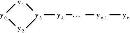
if nodes are encountered in subscript order. So worst case behavior is $O(n^{2})$.

The analysis above assumed that the degree of all nodes was bounded. Suppose not; suppose $\delta(y)\rightarrow n=|N|$. In this case the node $y$ will subsume many nodes, thereby bounding the number of necessary iterations. We have no formal proof for this last assertion, but it appears to be true.

Using their H-graph structure, Lin, Soulignac and Szwarcfiter, show that the cost to dismantle a network is $O(n+\alpha m)$ where $\alpha$ denotes the arboricity of ${\cal N}$ [12]. Experimentally, our reduction, $\omega$, of the Newman collaboration graph to its irreducible spine shown in Figure 3 required 5 iterations, with the last over the remaining 65 nodes to verify irreducibility. Other reductions of 4,764, and 5,242, node networks to their 228, and 1,469, node irreducible spines respectively took 5 and 6 iterations. In practice, network reduction appears to be nearly linear.

A cycle is a closed, simple path [2, 9]. A cycle $C=<y_{1},y_{2},\ldots,y_{k},y_{1}>$ has length $k$. For each node $y_{i}\in C$, $|\{y_{i}\}.\mbox{$\eta$}|\geq 2$. The irreducible spine of Figure 3 has an abundance of cycles and no nodes $x$ with $|\{x\}.\mbox{$\eta$}|=1$.

A chord in a cycle is an edge/connection $(y_{i},y_{j})\in E$ where $j\neq i\pm 1$ (or $i=1,j=k-1$). A cycle $C$ is chordless if it has no chords.⁴⁴ 4 In [15, 16], the author mistakenly used the term “fundamental cycle” for the chordless cycles that will be explored in this section.

It is the thesis of this paper that these chordless $k$-cycles provide a valuable characterization of the structure of a network. As a small example, consider Figure 5 from Granovetter’s 1973 article on ”weak ties” [8], which has been redrawn so as to emphasize the chordless 14-cycle.

The nodes $X,Y,Z$ represent other portions of the network. Readily, describing this subset as a 14-cycle with 9 pendant nodes is an appropriate characterization. Our goal with this example is simply to show that these kinds of chordless cycles arise naturally in the literature and in real life.

One should have many tools on hand to understand the nature of large graphs, or networks. In this paper we have presented one that is rather unusual, yet also rather powerful. Even so, it must be observed that the reduction, $\omega$, of graphs will always be of mixed value. Some graphs, for example chordal graphs, will reduce to a single node. This in itself conveys considerable information, but in this case other kinds of analysis are clearly more appropriate. Nevertheless, for many of the kinds of networks one encounters in real situations, reducing the network to its irreducible spine is a quick, easy first step.

Because the irreducible spine, ${\cal I}$, is effectively unique, further analysis of it is a valid way of getting information about the original network. It is a “reliable” surrogate. It preserves connectivity and path centrality concepts. Consequently, this kind of analysis with respect to closed sets can provide valuable insights into the nature, and the structure, of the network.

We believe that by counting edges as well as nodes in the subsumed chordal portions we can get much tighter bounds on the diameters and triangle counts in these subgraphs, and thus in the entire network. This, and further exploration of the idea of connective complexity are some of future research projects arising from this work.

References

- [1] Charu C. Aggarwal and Haixun Wang. On Dimensionality Reduction of Massive Graphs for Indexing and Retrieval. In Serge Abiteboul, Klemens Böhem, Christof Koch, and Kian-Lee Tan, editors, IEEE, 27th Intern. Conf. on Data Engineering (ICDE), pages 1091–1102, Hanover Germany, 2011.
- [2] Geir Agnarsson and Raymond Greenlaw. Graph Theory: Modeling, Applications and Algorithms. Prentice Hall, Upper Saddle River, NJ, 2007.
- [3] Ulrik Brandes. A Faster Algorithm for Betweeness Centrality. J.Mathematical Sociology, 25(2):163–177, 2001.
- [4] Thomas H. Cormen, Charles E. Leiserson, and Ronald L. Rivest. Introduction to Algorithms. MIT Press, Cambridge, MA, 1996.
- [5] Linton C. Freeman. Centrality in Social Networks, Conceptual Clarification. Social Networks, 1:215–239, 1978/79.
- [6] Linton C. Freeman. Visualizing Social Networks. J. of Social Structure, 1(1):1–19, 2000.
- [7] Anna C. Gilbert and Kirill Levchenko. Compressing Network Graphs. In Proc. LinkKDD’04, Seattle, WA, Aug. 2004.
- [8] Mark S. Granovetter. The Strength of Weak Ties. Amer. J. of Sociology, 78(6):1360–1380, 1973.
- [9] Frank Harary. Graph Theory. Addison-Wesley, 1969.
- [10] Michael S. Jacobson and Ken Peters. Chordal graphs and upper irredundance, upper domination and independence. Discrete Mathematics, 86(1-3):59–69, Dec. 1990.
- [11] Jure Leskovec and Christos Faloutsos. Sampling from Large Graphs. In 12th Intern. Conf. on Knowledge Discovery and Data Mining, KDD’06, pages 631–636, Philadelphia, PA, 2006.
- [12] Min Chin Lin, Francisco J. Soulignac, and Jayme L. Szwarcfiter. Arboricity, -Index, and Dynamic Algorithms. arXiv:1005.2211v1, pages 1–19, May 2010.
- [13] Terry A. McKee. How Chordal Graphs Work. Bulletin of the ICA, 9:27–39, 1993.
- [14] Mark. E. J. Newman. Finding community structure in networks using the eigenvectors of matrices. Phys.Rev.E, 74(036104):1–22, July 2006.
- [15] John L. Pfaltz. Mathematical Continuity in Dynamic Social Networks. In Anwitaman Datta, Stuart Shulman, Baihua Zheng, Shoude Lin, Aixin Sun, and Ee-Peng Lim, editors, Third International Conf. on Social Informatics, SocInfo2011, volume LNCS # 6984, pages 36–50, 2011.
- [16] John L. Pfaltz. Finding the Mule in the Network. In Reda Alhajj and Bob Werner, editors, Intern. Conf on Advances in Social Network Analysis and Mining, ASONAM 2012, pages 667–672, Istanbul, Turkey, August 2012.
- [17] Charalampos E. Tsourakakis, Petros Drineas, Eirinaios Michelakis, Ioannis Koutis, and Christos Faloutos. Spectral counting of triangles via element-wise sparsification and triangle-based link recommendation. Soc. Network Analysis and Mining, 1(2):75–81, Apr. 2011.