Finite size effects in the correlation structure of stochastic neural networks: analysis of different connectivity matrices and failure of the mean-field theory

Diego Fasoli* Olivier Faugeras*

*NeuroMathComp Laboratory, INRIA Sophia-Antipolis, France. Email: firstname.name@inria.fr

Abstract

We quantify the finite size effects in a stochastic network made up of rate neurons, for several kinds of recurrent connectivity matrices.

This analysis is performed by means of a perturbative expansion of the neural equations, where the perturbative parameters are the intensities of the sources of randomness in the system.

In detail, these parameters are the variances of the background or input noise, of the initial conditions and of the distribution of the synaptic weights.

The technique developed in this article can be used to study systems which are invariant under the exchange of the neural indices and it allows us to quantify the correlation structure of the network, in terms of pairwise and higher order correlations between the neurons.

We also determine the relation between the correlation and the external input of the network, showing that strong signals coming from the environment reduce significantly the amount of correlation between the neurons.

Moreover we prove that in general the phenomenon of propagation of chaos does not occur, even in the thermodynamic limit, due to the correlation structure of the $3$ sources of randomness considered in the model.

Furthermore, we show that the propagation of chaos does not depend only on the number of neurons in the network, but also and mainly on the number of incoming connections per neuron.

To conclude, we prove that for special values of the parameters of the system the neurons become perfectly correlated, a phenomenon that we have called stochastic synchronization.

These discoveries clearly prevent the use of the mean-field theory in the description of the neural network.

1 Introduction

According to the theory of complexity [1][2][3], in order to have emergent behaviors in systems made up of many interacting units, what really matters are not the properties of the single units themselves, but rather the way they interact with each other.

The most famous example of this phenomenon is represented by flocks of birds, since it is possible to recreate in a computer simulation their ability to form stable and complicated patterns and to rejoin when the group is splitted, throught the implementation of very simple rules of interaction.

In fact, according to the famous artificial life program Boids [4], it is possible to reproduce this emergent behavior assuming that every bird has to fly in the same direction of the neighbours, with the same speed and avoiding obstacles or to bump into other birds.

This example clearly shows that the complexity of the system is a consequence of the interaction between birds, and not of the model used to described a single bird.

Therefore, in the context of the brain, where the elementary units are represented by neurons, the priority is not to study extremely biologically realistic models of single neurons.

The really important problem is to describe in an accurate way the interaction between them, or in other terms their synaptic connectivity matrix.

For this reason we believe that it should be more relevant to use simplified neural models (like the so called rate model [5][6][7][8][9]) with complex connectivity matrices, than to use more biologically plausible neural models (like the Hodgkin-Huxley model [10]) with simple connections.

So in this article we focus mainly on the differences in the behavior of the network induced by different topologies of the synaptic connectivity.

Following this current of thought, a great effort has been devoted to finding the pattern of the synaptic connections of the human brain [11][12][13].

Therefore an important question we have to try to answer is: how does the behavior of the brain change when we modify its connectivity matrix?

This is the key to understand how the brain processes the information it receives from the environment, and hopefully also the necessary ingredient to explain how its higher cognitive functions naturally emerge from the interaction of the neurons.

It is therefore fundamental to develop a theory that is able to determine the behavior of a neural network once its external inputs and connectivity matrix are known, for many different kinds of input and connection structures.

The behavior of a neural network that this theory must be able to describe is twofold.

In fact the theory has to provide the time evolution of the membrane potentials and firing rates of the neurons but, from a probabilistic point of view, it must also be able to determine their statistics.

It is well known that the neurons are not reliable units and that the variability of their behavior is described by adding a source of stochasticity in their equations [14][15][16].

This transforms the system into a non-deterministic network, and therefore one has to compute the probability density of the neurons and their pairwise correlation structure.

Actually the latter is receiving an increasing attention from the scientific community since it may be involved in the extraordinary information processing capabilities of the brain.

It is also known as functional connectivity, a term coined in order to distinguish the correlation structure from the wiring pattern of all the synaptic connections, that is known instead as structural or anatomical connectivity.

The problem of finding the relation between these two kinds of connectivity is currently intensively investigated [17][18][19][20][21][22], and the theory we are looking for should provide such a link.

In Section 2 we develop a perturbative approch that let us determine the behavior of a neural network with finite size, made up of a generic number of neurons described by rate equations.

The perturbative parameters are the variances of the $3$ sources of randomness considered in the model: the background or input noise, the initial conditions and the synaptic weights.

This allows us to study the network for many different types of structural connectivity matrices, with a special emphasis on the evaluation of their corresponding functional connectivity matrices.

Therefore in Section 3 we provide an explicit formula that relates the two connectivity matrices, for many different kinds of structural connectivities, and we also explain how to use this model to compute higher order correlations, like those between triplets and quadruplets of neurons.

In particular, in Section 4 we consider the special cases of block circulant matrices with circulant blocks, and of symmetric matrices.

The goodness of the perturbative approach is proved in Section 5 through many numerical simulations.

Moreover, using these formulae, in Section 6 we determine the relation between the correlation structure and the external input of the network, showing that strong signals coming from the environment reduce significantly the amount of correlation between the neurons.

Moreover in Section 7 we prove that the phenomenon known as propagation of chaos [9][23][24][25] in general does not occur, even in the thermodynamic limit, due to the correlation structure of the $3$ sources of randomness.

Furthermore, we show that propagation of chaos does not depend only on the number of neurons in the network, but also and mainly on the number of incoming connections per neuron.

This model predicts also arbitrarily high values of correlation between the neurons for special values of the parameters of the system, a phenomenon that we have called stochastic synchronization.

The direct consequence of these results is therefore the impossibility to apply in general the mean-field theory in order to describe the activity of the network.

It is also interesting to observe that since this approach works for a generic and finite number of neurons $N$ , it is able to quantify the finite size effects of the network.

Therefore simply increasing the value of the parameter $N$ , in principle we can evaluate the differences that occur in the behavior of a neural network when we switch from a microscopic scale ( $N\sim 10^{0}$ , i.e. single neurons) to mesoscopic ( $N\sim 10^{1}\div 10^{5}$ , i.e. neural masses and cortical columns) and then to macroscopic scales ( $N\sim 10^{6}\div 10^{11}$ , i.e. extended brain areas, like the visual cortex).

This in principle would allow us to show if there are actually emerging properties of the system that are triggered by its size.

Such properties can be identified for example in a difference in the information processing capabilities of the system that emerges when we increase $N$ .

These capabilities can be evaluated with our model in the linear approximation regime, since in that case the system is described by a multivariate normal distribution and therefore it allows us to compute analytically all the information quantities of the system.

However we will not show this analysis here since it is beyond the purpose of the current article and also because the study of macroscopic areas of the brain requires the refinement of the model using neural fields equations [8][26][27] in order to describe the spatial extension of the areas and also the delays in the propagation of the electric signals.

2 Description of the model

We suppose that the neural network is described by the following rate model:

dV_{i}\left(t\right)=\left[-\frac{1}{\tau}V_{i}\left(t\right)+\sum_{j=0}^{N-1}J_{ij}\left(t\right)S\left(V_{j}\left(t\right)\right)+I_{i}\left(t\right)\right]dt+\sigma_{1}dB_{i}\left(t\right)

(2.1)

with $i=0,1,...,N-1$ .

Here $V_{i}\left(t\right)$ is the mebrane potential of the $i$ -th neuron, $I_{i}\left(t\right)$ is its external input current and $\tau$ is a time constant that determines the speed of convergence of the membrane potential to its rest state $V_{i}\left(t\right)=0$ in the case of disconnected neurons.

Moreover $N$ is the number of neurons in the network, $J_{ij}\left(t\right)$ is the synaptic weight from the the $j$ -th neuron to the $i$ -th neuron, and $S\left(\cdot\right)$ is a sigmoid function, which converts the membrane potential of a neuron into the rate of the spikes it produces, according to the law:

S\left(V\right)=\frac{T_{MAX}}{1+e^{-\lambda\left(V-V_{T}\right)}}

where $T_{MAX}$ is the maximum amplitude of the function, $\lambda$ is a parameter that determines its slope, and $V_{T}$ is the horizontal shift along the $V$ axis.

$\sigma_{1}$ is the noise intensity, that for simplicity is supposed to be the same for all the neurons and constant in time.

The functions $B_{i}\left(t\right)$ are Brownian motions, which can be equivalently interpreted as a background noise for the membrane potentials $V_{i}\left(t\right)$ or as the stochastic component of the external input $I_{i}\left(t\right)$ .

In general they are correlated according to a covariance matrix $\Sigma_{1}$ , whose components are:

	$\displaystyle\left[\Sigma_{1}\right]_{ij}=$	$\displaystyle Cov\left(\frac{dB_{i}\left(t\right)}{dt},\frac{dB_{j}\left(s\right)}{ds}\right)=C_{ij}^{1}\delta\left(t-s\right)$
	$\displaystyle C_{ij}^{1}=$	$\displaystyle\begin{cases}1&\begin{array}[]{ccc}\mathrm{if}&&i=j\end{array}\\ \\ C_{1}&\begin{array}[]{ccc}\mathrm{if}&&i\neq j\end{array}\end{cases}$

where $\delta\left(\cdot\right)$ is the Dirac delta function, while $C_{1}$ represents the correlation between two different Brownian motions (here the derivative of the Brownian motion is meant in the weak sense of distributions and is interpreted as white noise). In order to be a true covariance matrix, $\Sigma_{1}$ must be positive-semidefinite. Since it is symmetric, then it is positive-semidefinite if and only if its eigenvalues are non-negative. But $\Sigma_{1}$ is a circulant matrix, therefore its eigenvalues are $e_{0}=1+C_{1}\left(N-1\right)$ and $e_{i}=1-C_{1}$ , for $i=1,2,...,N-1$ . Therefore $\Sigma_{1}$ is positive-semidefinite if and only if $\frac{1}{1-N}\leq C_{1}\leq 1$ . We could increase the complexity of this correlation structure, since there is no technical difficulty in doing that, but we keep it simple for the sake of clarity.

We also suppose that the initial conditions are distributed according to the following multivariate normal probability density:

\overrightarrow{V}\left(0\right)\sim\mathcal{N}\left(\overrightarrow{\mu},\Sigma_{2}\right)

(2.3)

where for simplicity:

	$\displaystyle\mu_{i}=$	$\displaystyle\begin{array}[]{ccc}\mu,&&i=0,1,...,N-1\end{array}$
	$\displaystyle\Sigma_{2}=$	$\displaystyle\sigma_{2}^{2}\left[\begin{array}[]{cccc}1&C_{2}&\cdots&C_{2}\\ C_{2}&1&\cdots&C_{2}\\ \vdots&\vdots&\ddots&\vdots\\ C_{2}&C_{2}&\cdots&1\end{array}\right]$

Here $\sigma_{2}$ represents the initial standard deviation of each neuron, while $C_{2}$ is the initial correlation between pairs of neurons. As before, the matrix $\Sigma_{2}$ must be positive-semidefinite, and this is true if and only if $\frac{1}{1-N}\leq C_{2}\leq 1$ . Again, we could increase the complexity of this correlation structure, if desired.

For the synaptic connectivity matrix $J\left(t\right)$ , we suppose that its entries have a deterministic temporal evolution, but they are distributed randomly over many repetitions of the network. With this model we can match our results with those appeared in [28]. So, in detail, we suppoose that the synaptic connectivity matrix $J\left(t\right)$ has random entries distributed according to the law:

J\left(t\right)\sim\mathcal{MN}\left(\overline{J}+\sigma_{4}Z\left(t\right),\Omega_{3},\Sigma_{3}\right)

(2.9)

This is the so called matrix normal distribution [29], namely the generalization of the multivariate normal distribution to the case of matrix-valued random variables. Here $\overline{J}$ , $Z\left(t\right)$ , $\Omega_{3}$ and $\Sigma_{3}$ are $N\times N$ deterministic matrices. In particular, $\overline{J}+\sigma_{4}Z\left(t\right)$ represents the mean of $J\left(t\right)$ , while $\Omega_{3}$ and $\Sigma_{3}$ are its covariance matrices. We suppose that $\overline{J}$ has only two different kinds of entries, namely $0$ (absence of connection) and $\Lambda$ , where $\Lambda$ is a free non-zero parameter. We also suppose that $Z\left(t\right)$ has general entries (with the obvious exception that $Z_{ij}\left(t\right)=0$ if there is no connection from the $j$ -th neuron to the $i$ -th neuron, namely if $J_{ij}\left(t\right)=0$ $\forall t$ ), therefore it is a source of inhomogeneity and time-variability for the connectivity matrix. We use for simplicity specific structures of the covariance matrices $\Omega_{3}$ and $\Sigma_{3}$ . Supposing that all the non-zero entries of $J\left(t\right)$ have the same standard deviation $\sigma_{3}$ , it is possible to rewrite the matrix $J\left(t\right)$ in the following equivalent way:

	$\displaystyle J\left(t\right)=$	$\displaystyle\overline{J}+\sigma_{3}W+\sigma_{4}Z\left(t\right)$		(2.10)
	$\displaystyle W\sim$	$\displaystyle\mathcal{MN}\left(0,\widetilde{\Omega}_{3},\widetilde{\Sigma}_{3}\right)$		(2.11)

where $\widetilde{\Omega}_{3}$ and $\widetilde{\Sigma}_{3}$ are normalized covariance matrices. Their explicit structure is not important, and the only thing that we need to know is that they are chosen in order to have:

Cov\left(W_{ij},W_{kl}\right)=\begin{cases}0&\begin{array}[]{ccc}\mathrm{if}&&\left(g\left(i,j\right)=0\right)\vee\left(g\left(k,l\right)=0\right)\end{array}\\ \\ 1&\begin{array}[]{ccc}\mathrm{if}&&\left(i=k\right)\wedge\left(j=l\right)\wedge\left(g\left(i,j\right)=1\right)\end{array}\\ \\ C_{3}&\mathrm{otherwise}\end{cases}

(2.12)

where $g\left(x,y\right)=0$ if there is no synaptic connection from the the $y$ -th neuron to the $x$ -th neuron (namely if $J_{xy}\left(t\right)=0$ $\forall t$ ), and $1$ otherwise, while $C_{3}$ is the correlation between two different and non-zero synaptic weights. We observe that the range of the possible values of $C_{3}$ in general depends on the topology of the connectivity matrix, and $W_{ij}=0$ if there is no connection from the $j$ -th neuron to the $i$ -th neuron (this is a consequence of the formulae 2.10 and 2.12). Again, as for the Brownian motions and the initial conditions, we could increase the complexity of this correlation structure, if desired.

We suppose that every neuron has the same number of incoming connections, that we call $M$ . We observe that our assumptions imply that the network is invariant under exchange of the neuronal indices, which is the main hypothesis of this article. When $M$ increases, each neuron receives a larger and larger input from the remainder of the network, therefore in order to fix this divergence we normalize the synaptic weight in the following way:

J\left(t\right)\rightarrow\frac{J\left(t\right)}{M}

This normalization is intended to be used only when $M\neq 0$ , because otherwise we obtain $J_{ij}=\frac{0}{0}$ . For $M=0$ the neurons have no incoming connections, therefore we have simply to set $J_{ij}=0$ .

To conclude, we also suppose that the external input current is deterministic (if we interpret $B_{i}\left(t\right)$ as the noise of the membrane potential) and given by:

\overrightarrow{I}\left(t\right)=\overrightarrow{\overline{I}}+\sigma_{5}\overrightarrow{H}\left(t\right)

(2.13)

where the vector $\overrightarrow{\overline{I}}$ is time-independent and such that $\overline{I}_{i}=\overline{I}$ , for $i=0,1,...,N-1$ . The vector $\overrightarrow{H}\left(t\right)$ has in general different and time-variable entries, so it is a source of inhomogeneity and time-variability.

Now we define the following 2nd order perturbative expansion of the membrane potential:

V_{i}\left(t\right)\approx\mu+\sum_{m=1}^{5}\sigma_{m}Y_{m}^{i}\left(t\right)+{\displaystyle\sum\limits_{\begin{subarray}{c}m,n=1\\ m\leq n\end{subarray}}^{5}}\sigma_{m}\sigma_{n}Y_{m,n}^{i}\left(t\right)

(2.14)

which will be used to obtain an approximate analytic solution of the system 2.1.

2.1 The system of equations

Now we put the perturbative expansion 2.14 and the expressions 2.10 and 2.13 for, respectively, the synaptic weights and the external input current, inside the system 2.1. If all the parameters $\sigma_{m}$ are small enough, we can expand the sigmoid function in a Taylor series around $\mu$ (see 2). In order to be rigorous, we have to determine the radius of convergence of the Taylor expansion of $S\left(V\right)$ for every value of $V$ and to check if it is big enough compared to $\sigma_{m}$ , because otherwise our technique cannot be applied. In fact, the various $\sigma_{m}$ determine the order of magnitude of the fluctuations of $V$ around $\mu$ , therefore it is important to check that $V$ is inside the interval of convergence of the Taylor expansion of $S\left(V\right)$ . To our knowledge, this calculation has been performed only for $V=0$ , so in Appendix A we show the general analysis, obtaining that in general the radius of convergence decreases with the slope parameter $\lambda$ of the sigmoid function. So, supposing that $\lambda$ is small enough, if we call:

\zeta_{j}=\sum_{m=1}^{5}\sigma_{m}Y_{m}^{j}\left(t\right)+{\displaystyle\sum\limits_{\begin{subarray}{c}m,n=1\\ m\leq n\end{subarray}}^{5}}\sigma_{m}\sigma_{n}Y_{m,n}^{j}\left(t\right)

the Taylor expansion of the sigmoid function is:

\displaystyle S\left(\mu+\zeta_{j}\right)\approx

\displaystyle S\left(\mu\right)+S^{\prime}\left(\mu\right)\zeta_{j}+\frac{1}{2}S^{\prime\prime}\left(\mu\right)\zeta_{j}^{2}\hphantom{\,\,\,\,\,\,\,\,\,\,\,\,\,\,\,\,\,\,\,\,\,\,\,\,\,\,\,\,\,\,\,\,\,\,\,\,\,\,\,\,\,\,\,\,\,\,\,\,\,\,\,\,\,\,\,\,\,\,\,\,\,\,\,\,\,\,\,\,\,\,\,\,\,\,\,\,\,\,\,\,\,\,\,\,\,\,\,\,\,\,\,\,\,}

	$\displaystyle\approx$	$\displaystyle S\left(\mu\right)+S^{\prime}\left(\mu\right)\sum_{m=1}^{5}\sigma_{m}Y_{m}^{j}\left(t\right)$
		$\displaystyle+{\displaystyle\sum\limits_{\begin{subarray}{c}m,n=1\\ m<n\end{subarray}}^{5}}\sigma_{m}\sigma_{n}\left[S^{\prime}\left(\mu\right)Y_{m,n}^{j}\left(t\right)+S^{\prime\prime}\left(\mu\right)Y_{m}^{j}\left(t\right)Y_{n}^{j}\left(t\right)\right]$
		$\displaystyle+\sum_{m=1}^{5}\sigma_{m}^{2}\left[S^{\prime}\left(\mu\right)Y_{m,m}^{j}\left(t\right)+\frac{1}{2}S^{\prime\prime}\left(\mu\right)\left(Y_{m}^{j}\left(t\right)\right)^{2}\right]$

having neglected the terms with order higher than $2$ . Now we substitute this expansion of the sigmoid function inside the neural equation system and we equate the terms with the same $\sigma$ coefficients, obtaining (here we report only the equations that we will actually use to compute the correlation structure in Section 3):

$\displaystyle\mu=$	$\displaystyle\tau\left[\Lambda S\left(\mu\right)+\overline{I}\right]$	(2.15)
$\displaystyle dY_{1}^{i}\left(t\right)=$	$\displaystyle\left[-\frac{1}{\tau}Y_{1}^{i}\left(t\right)+S^{\prime}\left(\mu\right)\sum_{j=0}^{N-1}\overline{J}_{ij}Y_{1}^{j}\left(t\right)\right]dt+dB_{i}\left(t\right)$	(2.16)
$\displaystyle dY_{2}^{i}\left(t\right)=$	$\displaystyle\left[-\frac{1}{\tau}Y_{2}^{i}\left(t\right)+S^{\prime}\left(\mu\right)\sum_{j=0}^{N-1}\overline{J}_{ij}Y_{2}^{j}\left(t\right)\right]dt$	(2.17)
$\displaystyle dY_{3}^{i}\left(t\right)=$	$\displaystyle\left[-\frac{1}{\tau}Y_{3}^{i}\left(t\right)+S^{\prime}\left(\mu\right)\sum_{j=0}^{N-1}\overline{J}_{ij}Y_{3}^{j}\left(t\right)+S\left(\mu\right)\sum_{j=0}^{N-1}W_{ij}\right]dt$	(2.18)
$\displaystyle dY_{4}^{i}\left(t\right)=$	$\displaystyle\left[-\frac{1}{\tau}Y_{4}^{i}\left(t\right)+S^{\prime}\left(\mu\right)\sum_{j=0}^{N-1}\overline{J}_{ij}Y_{4}^{j}\left(t\right)+S\left(\mu\right)\sum_{j=0}^{N-1}Z_{ij}\left(t\right)\right]dt$	(2.19)
$\displaystyle dY_{5}^{i}\left(t\right)=$	$\displaystyle\left[-\frac{1}{\tau}Y_{5}^{i}\left(t\right)+S^{\prime}\left(\mu\right)\sum_{j=0}^{N-1}\overline{J}_{ij}Y_{5}^{j}\left(t\right)+H_{i}\left(t\right)\right]dt\hphantom{\,\,\,\,\,\,\,\,\,\,\,\,\,\,\,\,\,\,\,\,\,\,\,\,\,\,\,\,\,\,\,\,\,\,\,\,\,\,\,\,\,\,\,\,\,\,\,\,\,\,\,\,\,\,\,\,\,\,\,\,\,\,\,\,\,\,\,\,\,\,\,\,\,\,\,\,\,\,\,\,\,\,\,\,\,\,\,\,\,\,\,\,\,\,\,\,\,\,\,\,\,\,\,\,\,\,\,\,\,\,\,\,\,\,\,\,\,\,\,\,\,\,\,\,\,\,\,\,\,\,\,\,\,\,\,\,}$	(2.20)

$\displaystyle dY_{1,4}^{i}\left(t\right)=$	$\displaystyle\left[-\frac{1}{\tau}Y_{1,4}^{i}\left(t\right)+S^{\prime}\left(\mu\right)\sum_{j=0}^{N-1}\overline{J}_{ij}Y_{1,4}^{j}\left(t\right)+S^{\prime}\left(\mu\right)\sum_{j=0}^{N-1}Z_{ij}\left(t\right)Y_{1}^{j}\left(t\right)+S^{\prime\prime}\left(\mu\right)\sum_{j=0}^{N-1}\overline{J}_{ij}Y_{1}^{j}\left(t\right)Y_{4}^{j}\left(t\right)\right]dt$	(2.21)
$\displaystyle dY_{1,5}^{i}\left(t\right)=$	$\displaystyle\left[-\frac{1}{\tau}Y_{1,5}^{i}\left(t\right)+S^{\prime}\left(\mu\right)\sum_{j=0}^{N-1}\overline{J}_{ij}Y_{1,5}^{j}\left(t\right)+S^{\prime\prime}\left(\mu\right)\sum_{j=0}^{N-1}\overline{J}_{ij}Y_{1}^{j}\left(t\right)Y_{5}^{j}\left(t\right)\right]dt$	(2.22)
$\displaystyle dY_{2,4}^{i}\left(t\right)=$	$\displaystyle\left[-\frac{1}{\tau}Y_{2,4}^{i}\left(t\right)+S^{\prime}\left(\mu\right)\sum_{j=0}^{N-1}\overline{J}_{ij}Y_{2,4}^{j}\left(t\right)+S^{\prime}\left(\mu\right)\sum_{j=0}^{N-1}Z_{ij}\left(t\right)Y_{2}^{j}\left(t\right)+S^{\prime\prime}\left(\mu\right)\sum_{j=0}^{N-1}\overline{J}_{ij}Y_{2}^{j}\left(t\right)Y_{4}^{j}\left(t\right)\right]dt$	(2.23)
$\displaystyle dY_{2,5}^{i}\left(t\right)=$	$\displaystyle\left[-\frac{1}{\tau}Y_{2,5}^{i}\left(t\right)+S^{\prime}\left(\mu\right)\sum_{j=0}^{N-1}\overline{J}_{ij}Y_{2,5}^{j}\left(t\right)+S^{\prime\prime}\left(\mu\right)\sum_{j=0}^{N-1}\overline{J}_{ij}Y_{2}^{j}\left(t\right)Y_{5}^{j}\left(t\right)\right]dt$	(2.24)
$\displaystyle dY_{3,4}^{i}\left(t\right)=$	$\displaystyle\left[-\frac{1}{\tau}Y_{3,4}^{i}\left(t\right)+S^{\prime}\left(\mu\right)\sum_{j=0}^{N-1}\overline{J}_{ij}Y_{3,4}^{j}\left(t\right)+S^{\prime}\left(\mu\right)\sum_{j=0}^{N-1}Z_{ij}\left(t\right)Y_{3}^{j}\left(t\right)\right.$
	$\displaystyle\left.+S^{\prime}\left(\mu\right)\sum_{j=0}^{N-1}W_{ij}Y_{4}^{j}\left(t\right)+S^{\prime\prime}\left(\mu\right)\sum_{j=0}^{N-1}\overline{J}_{ij}Y_{3}^{j}\left(t\right)Y_{4}^{j}\left(t\right)\right]dt$	(2.25)
$\displaystyle dY_{3,5}^{i}\left(t\right)=$	$\displaystyle\left[-\frac{1}{\tau}Y_{3,5}^{i}\left(t\right)+S^{\prime}\left(\mu\right)\sum_{j=0}^{N-1}\overline{J}_{ij}Y_{3,5}^{j}\left(t\right)+S^{\prime}\left(\mu\right)\sum_{j=0}^{N-1}W_{ij}Y_{5}^{j}\left(t\right)+S^{\prime\prime}\left(\mu\right)\sum_{j=0}^{N-1}\overline{J}_{ij}Y_{3}^{j}\left(t\right)Y_{5}^{j}\left(t\right)\right]dt$	(2.26)

Equation 2.15 is algebraic and non-linear, therefore must be solved numerically. 2.16 is the only stochastic differential equation of the set and can be solved analytically, since it is linear with constant coefficients. Equations 2.17 - 2.20 are ordinary, and can be solved in the same way as 2.16. To conclude, equations 2.21 - 2.26 determine the functions $Y_{m,n}^{i}\left(t\right)$ , and depend on the terms $Y_{m}^{i}\left(t\right)$ , which have been calculated at the previous step. Being linear and with constant coefficients, they can be integrated analytically as a function of the already known functions $Y_{m}^{i}\left(t\right)$ .

2.2 The initial conditions

The perturbative expansion 2.14 at $t=0$ gives:

V_{i}\left(0\right)\approx\mu+\sum_{m=1}^{5}\sigma_{m}Y_{m}^{i}\left(0\right)+{\displaystyle\sum\limits_{\begin{subarray}{c}m,n=1\\ m\leq n\end{subarray}}^{5}}\sigma_{m}\sigma_{n}Y_{m,n}^{i}\left(0\right)

Moreover, according to 2.3, we have $V_{i}\left(0\right)\sim\mathcal{N}\left(\mu,\sigma_{2}^{2}\right)=\mu+\sigma_{2}\mathcal{N}\left(0,1\right)$ , so from the comparison it must be:

		$\displaystyle Y_{2}^{i}\left(0\right)\sim\mathcal{N}\left(0,1\right)$		(2.27)
		$\displaystyle\begin{array}[]{ccc}Y_{m}^{i}\left(0\right)=0,&&m=1,3,4,5\end{array}$
		$\displaystyle\begin{array}[]{ccc}Y_{m,n}^{i}\left(0\right)=0,&&\forall\left(m,n\right):\,m\leq n\end{array}$

So we have $V_{i}\left(0\right)=\mu+\sigma_{2}Y_{2}^{i}\left(0\right)$ and therefore:

Cov\left(V_{i}\left(0\right),V_{j}\left(0\right)\right)=\sigma_{2}^{2}Cov\left(Y_{2}^{i}\left(0\right),Y_{2}^{j}\left(0\right)\right)

But from 2 we also know that:

Cov\left(V_{i}\left(0\right),V_{j}\left(0\right)\right)=\begin{cases}\sigma_{2}^{2}&\begin{array}[]{ccc}\mathrm{if}&&i=j\end{array}\\ \\ \sigma_{2}^{2}C_{2}&\begin{array}[]{ccc}\mathrm{if}&&i\neq j\end{array}\end{cases}

so from the comparison it must be that:

Cov\left(Y_{2}^{i}\left(0\right),Y_{2}^{j}\left(0\right)\right)=\begin{cases}1&\begin{array}[]{ccc}\mathrm{if}&&i=j\end{array}\\ \\ C_{2}&\begin{array}[]{ccc}\mathrm{if}&&i\neq j\end{array}\end{cases}

(2.30)

2.3 Solutions of the equations

As we said at the end of Section 2.1, the algebraic equation 2.15 is non-linear, therefore it cannot be solved exactly. However, the differential equations satisfied by all the functions $Y_{m}^{i}\left(t\right)$ and $Y_{m,n}^{i}\left(t\right)$ are linear with constant coefficients, therefore they can be solved analytically. In particular, the equations 2.16 - 2.20 can be solved directly. Instead the remaining equations are functions of the previous $Y_{m}^{i}\left(t\right)$ , that we have already calculated. For example, according to 2.21, $Y_{1,4}^{i}\left(t\right)$ can be determined analytically as a function of $Y_{1}^{i}\left(t\right)$ and $Y_{4}^{i}\left(t\right)$ , which are already known from the equations 2.16 and 2.19. Now we introduce the fundamental matrix $\Phi\left(t\right)$ such that:

	$\displaystyle\Phi\left(t\right)=$	$\displaystyle e^{At}$
	$\displaystyle A_{ij}=$	$\displaystyle\begin{cases}-\frac{1}{\tau}&\begin{array}[]{ccc}\mathrm{if}&&i=j\end{array}\\ \\ \overline{J}_{ij}S^{\prime}\left(\mu\right)&\begin{array}[]{ccc}\mathrm{if}&&i\neq j\end{array}\end{cases}$

where:

\mathcal{J}=\overline{J}S^{\prime}\left(\mu\right)

(2.32)

is the effective connectivity matrix of the network. Therefore the solutions of all the functions $Y_{m}^{i}\left(t\right)$ can be obtained straightforwardly as follows:

\displaystyle Y_{1}^{i}\left(t\right)=\sum_{j=0}^{N-1}\int_{0}^{t}\left[\Phi\left(t-s\right)\right]_{ij}dB_{j}\left(s\right)\hphantom{\,\,\,\,\,\,\,\,\,\,\,\,\,\,\,\,\,\,\,\,\,\,\,\,\,\,\,\,\,\,\,\,\,\,\,\,\,\,\,\,\,\,\,\,\,\,\,\,\,\,\,\,\,\,\,\,\,\,\,\,\,\,\,\,\,\,\,\,\,\,\,\,\,\,\,\,\,\,\,\,\,\,\,\,\,\,\,\,\,\,\,\,\,\,\,\,\,\,\,\,\,\,\,\,\,\,\,\,\,\,\,\,\,\,\,\,\,\,\,\,\,\,\,\,\,\,\,\,\,\,\,\,\,\,\,\,\,\,\,\,\,\,\,\,\,\,\,\,\,\,\,\,\,\,\,\,\,\,\,\,\,\,\,\,\,\,\,\,\,\,\,\,\,\,\,\,\,\,\,\,\,\,\,\,\,\,\,\,\,\,\,\,\,\,\,\,\,}

(2.33)

$\displaystyle Y_{2}^{i}\left(t\right)=$	$\displaystyle\sum_{j=0}^{N-1}\Phi_{ij}\left(t\right)Y_{2}^{j}\left(0\right)$	(2.34)
$\displaystyle Y_{3}^{i}\left(t\right)=$	$\displaystyle S\left(\mu\right)\sum_{j,k=0}^{N-1}W_{jk}\int_{0}^{t}\left[\Phi\left(t-s\right)\right]_{ij}ds$	(2.35)
$\displaystyle Y_{4}^{i}\left(t\right)=$	$\displaystyle S\left(\mu\right)\sum_{j,k=0}^{N-1}\int_{0}^{t}\left[\Phi\left(t-s\right)\right]_{ij}Z_{jk}\left(s\right)ds$	(2.36)
$\displaystyle Y_{5}^{i}\left(t\right)=$	$\displaystyle\sum_{j=0}^{N-1}\int_{0}^{t}\left[\Phi\left(t-s\right)\right]_{ij}H_{j}\left(s\right)ds$	(2.37)
$\displaystyle Y_{1,4}^{i}\left(t\right)=$	$\displaystyle S^{\prime}\left(\mu\right)\sum_{j,k,l=0}^{N-1}\int_{0}^{t}\left[\Phi\left(t-s\right)\right]_{ij}\left\{\int_{0}^{s}\left[\Phi\left(s-u\right)\right]_{kl}dB_{l}\left(u\right)\right\}Z_{jk}\left(s\right)ds$
	$\displaystyle+S\left(\mu\right)S^{\prime\prime}\left(\mu\right)\sum_{j,k,l,m,n=0}^{N-1}\overline{J}_{jk}\int_{0}^{t}\left[\Phi\left(t-s\right)\right]_{ij}\left\{\int_{0}^{s}\left[\Phi\left(s-u\right)\right]_{kl}dB_{l}\left(u\right)\right\}\left\{\int_{0}^{s}\left[\Phi\left(s-u\right)\right]_{km}Z_{mn}\left(u\right)du\right\}ds$	(2.38)
$\displaystyle Y_{1,5}^{i}\left(t\right)=$	$\displaystyle S^{\prime\prime}\left(\mu\right)\sum_{j,k,l,m=0}^{N-1}\overline{J}_{jk}\int_{0}^{t}\left[\Phi\left(t-s\right)\right]_{ij}\left\{\int_{0}^{s}\left[\Phi\left(s-u\right)\right]_{kl}dB_{l}\left(u\right)\right\}\left\{\int_{0}^{s}\left[\Phi\left(s-u\right)\right]_{km}H_{m}\left(u\right)du\right\}ds$	(2.39)
$\displaystyle Y_{2,4}^{i}\left(t\right)=$	$\displaystyle S^{\prime}\left(\mu\right)\sum_{j,k,l=0}^{N-1}Y_{2}^{l}\left(0\right)\int_{0}^{t}\left[\Phi\left(t-s\right)\right]_{ij}\Phi_{kl}\left(s\right)Z_{jk}\left(s\right)ds$
	$\displaystyle+S\left(\mu\right)S^{\prime\prime}\left(\mu\right)\sum_{j,k,l,m,n=0}^{N-1}\overline{J}_{jk}Y_{2}^{l}\left(0\right)\int_{0}^{t}\left[\Phi\left(t-s\right)\right]_{ij}\Phi_{kl}\left(s\right)\left\{\int_{0}^{s}\left[\Phi\left(s-u\right)\right]_{km}Z_{mn}\left(u\right)du\right\}ds$	(2.40)
$\displaystyle Y_{2,5}^{i}\left(t\right)=$	$\displaystyle S^{\prime\prime}\left(\mu\right)\sum_{j,k,l,m=0}^{N-1}\overline{J}_{jk}Y_{2}^{l}\left(0\right)\int_{0}^{t}\left[\Phi\left(t-s\right)\right]_{ij}\Phi_{kl}\left(s\right)\left\{\int_{0}^{s}\left[\Phi\left(s-u\right)\right]_{km}H_{m}\left(u\right)du\right\}ds$	(2.41)
$\displaystyle Y_{3,4}^{i}\left(t\right)=$	$\displaystyle S\left(\mu\right)S^{\prime}\left(\mu\right)\sum_{j,k,l,m=0}^{N-1}W_{lm}\int_{0}^{t}\left[\Phi\left(t-s\right)\right]_{ij}\left\{\int_{0}^{s}\left[\Phi\left(s-u\right)\right]_{kl}du\right\}Z_{jk}\left(s\right)ds$
	$\displaystyle+S\left(\mu\right)S^{\prime}\left(\mu\right)\sum_{j,k,l,m=0}^{N-1}W_{jk}\int_{0}^{t}\left[\Phi\left(t-s\right)\right]_{ij}\left\{\int_{0}^{s}\left[\Phi\left(s-u\right)\right]_{kl}Z_{lm}\left(u\right)du\right\}ds$
	$\displaystyle+S^{2}\left(\mu\right)S^{\prime\prime}\left(\mu\right)\sum_{j,k,l,m,n,p=0}^{N-1}\overline{J}_{jk}W_{lm}\int_{0}^{t}\left[\Phi\left(t-s\right)\right]_{ij}\left\{\int_{0}^{s}\left[\Phi\left(s-u\right)\right]_{kl}du\right\}\left\{\int_{0}^{s}\left[\Phi\left(s-u\right)\right]_{kn}Z_{np}\left(u\right)du\right\}ds$	(2.42)

	$\displaystyle Y_{3,5}^{i}\left(t\right)=$	$\displaystyle S^{\prime}\left(\mu\right)\sum_{j,k,l=0}^{N-1}W_{jk}\int_{0}^{t}\left[\Phi\left(t-s\right)\right]_{ij}\left\{\int_{0}^{s}\left[\Phi\left(s-u\right)\right]_{kl}H_{l}\left(u\right)du\right\}ds$
		$\displaystyle+S\left(\mu\right)S^{\prime\prime}\left(\mu\right)\sum_{j,k,l,m,n=0}^{N-1}\overline{J}_{jk}W_{lm}\int_{0}^{t}\left[\Phi\left(t-s\right)\right]_{ij}\left\{\int_{0}^{s}\left[\Phi\left(s-u\right)\right]_{kl}du\right\}\left\{\int_{0}^{s}\left[\Phi\left(s-u\right)\right]_{kn}H_{n}\left(u\right)du\right\}ds$		(2.43)

To conclude, we have performed a perturbative expansion around a stationary state $\mu$ because in this way the equations 2.16 - 2.26 have constant coefficients and therefore they can be solved exactly using the fundamental matrix . Had we performed the perturbative expansion around a non-stationary state, we would have obtained a system of differential equations with time-varying coefficients, whose general solution is not known. In this case, the best thing that we can try is to write the solution in terms of the Magnus expansion [30], but this introduces another approximation to the real solution of the neural network.

In this article we have also supposed that the system is invariant under exchange of the neural indices: for this reason we have used the same stationary solution $\mu$ , the same (unperturbed) input current $\overline{I}$ and the same number of incoming connections for all the neurons in the network. This invariance is required in order to ensure that the effective connectivity matrix $\mathcal{J}$ given by 2.32 has the same structure as the real and unperturbed connectivity matrix $\overline{J}$ . In this way the fundamental matrix $\Phi\left(t\right)$ can be calculated using the properties of $\overline{J}$ , as explained in Section 4. If the system is not invariant under exchange of the neural indices, $\mathcal{J}$ does not inherit the structure of $\overline{J}$ , therefore the technique introduced in this article cannot be used anymore (see also the discussion at the end of Section 4.2). To conclude, it is important to observe that even if we have chosen structures of $\Sigma_{1}$ , $\Sigma_{2}$ , $\Sigma_{3}$ and $\Omega_{3}$ that are invariant under exchange of the neural indices, their invariance is not required here: we have used it only to simplify the final formulae that we will obtain in Section 3. Therefore in principle inhomogeneous structures can be used for these covariance matrices.

3 Correlation structure of the network

In this section we want to calculate the correlation structure of the membrane potentials, according to the perturbative expansion 2.14. Since the covariance function is bilinear, we have to compute it for all the possible combinations of the pairs $\left(Y_{m}^{i}\left(t\right),Y_{n}^{j}\left(t\right)\right)$ , $\left(Y_{m}^{i}\left(t\right),Y_{n,p}^{j}\left(t\right)\right)$ and $\left(Y_{m,n}^{i}\left(t\right),Y_{p,q}^{j}\left(t\right)\right)$ . However we do not have to consider the terms of order $4$ , like $\sigma_{1}^{2}\sigma_{2}^{2}Cov\left(Y_{1,1}^{i}\left(t\right),Y_{2,2}^{j}\left(t\right)\right)$ , because they are incomplete. In effect, in the perturbative expansion of $V_{i}\left(t\right)$ , we did not consider the terms of order $3$ , like $\sigma_{1}^{2}\sigma_{2}Y_{1,1,2}^{i}\left(t\right)$ , that generate contributions of order $4$ in the formula of the covariance. So the terms of order $4$ cannot be considered in the expansion of the covariance, therefore the final formula is of order $3$ .

For simplicity we suppose that the Brownian motions, the initial conditions and the uncertainty of the synaptic weights are $3$ independent random processes (and indeed there is a priori no obvious reason to think that they are correlated), so all the cross terms like $\sigma_{1}\sigma_{2}Cov\left(Y_{1}^{i}\left(t\right),Y_{2}^{j}\left(t\right)\right)$ , $\sigma_{1}\sigma_{2}Cov\left(Y_{2}^{i}\left(t\right),Y_{1}^{j}\left(t\right)\right)$ , $\sigma_{1}^{2}\sigma_{3}Cov\left(Y_{1,1}^{i}\left(t\right),Y_{3}^{j}\left(t\right)\right)$ , … are equal to zero (however, if desired, we could assume non-zero correlations between these $3$ sources of randomness, since there is no technical difficulty in the calculations, only the problem to compute many non-zero cross terms). Let us show it with an example:

	$\displaystyle Cov\left(Y_{1}^{i}\left(t\right),Y_{2}^{j}\left(t\right)\right)=$	$\displaystyle Cov\left(\int_{0}^{t}\sum_{k=0}^{N-1}\left[\Phi\left(t-s\right)\right]_{ik}dB_{k}\left(s\right),\sum_{l=0}^{N-1}\Phi_{jl}\left(t\right)Y_{2}^{l}\left(0\right)\right)$
	$\displaystyle=$	$\displaystyle\sum_{k,l=0}^{N-1}\Phi_{jl}\left(t\right)Cov\left(\int_{0}^{t}\left[\Phi\left(t-s\right)\right]_{ik}dB_{k}\left(s\right),Y_{2}^{l}\left(0\right)\right)$
	$\displaystyle=$	$\displaystyle 0$

since $B_{k}\left(s\right)$ and $Y_{2}^{l}\left(0\right)$ are independent by assumption. Moreover, due to the Isserlis’ theorem [31], we obtain also that all the terms in the covariance proportional to $\sigma_{m}^{2}\sigma_{n}$ with $m,n=1,2,3$ are equal to zero, like $\sigma_{1}^{2}\sigma_{2}$ and $\sigma_{3}^{3}$ . The same thing happens to all the terms proportional to $\sigma_{m}^{2}\sigma_{n}$ , with $m=4,5$ and $n=1,2,3$ . This is due to the fact that, according to the Isserlis’ theorem again, the mean of the product of any odd number of zero-mean normal processes is equal to zero. We show it with an example:

		$\displaystyle Cov\left(Y_{2}^{i}\left(t\right),Y_{2,2}^{j}\left(t\right)\right)$
		$\displaystyle=Cov\left(\sum_{k=0}^{N-1}\Phi_{ik}\left(t\right)Y_{2}^{k}\left(0\right),\frac{1}{2}S^{\prime\prime}\left(\mu\right)\sum_{l,m,n,p=0}^{N-1}\overline{J}_{lm}Y_{2}^{n}\left(0\right)Y_{2}^{p}\left(0\right)\int_{0}^{t}\left[\Phi\left(t-s\right)\right]_{jl}\Phi_{mn}\left(s\right)\Phi_{mp}\left(s\right)ds\right)$
		$\displaystyle=\frac{1}{2}S^{\prime\prime}\left(\mu\right)\sum_{k,l,m,n,p=0}^{N-1}\Phi_{ik}\left(t\right)\overline{J}_{lm}\left\{\int_{0}^{t}\left[\Phi\left(t-s\right)\right]_{jl}\Phi_{mn}\left(s\right)\Phi_{mp}\left(s\right)ds\right\}Cov\left(Y_{2}^{k}\left(0\right),Y_{2}^{n}\left(0\right)Y_{2}^{p}\left(0\right)\right)$
		$\displaystyle=0$

because:

Cov\left(Y_{2}^{k}\left(0\right),Y_{2}^{n}\left(0\right)Y_{2}^{p}\left(0\right)\right)=\mathbb{E}\left[Y_{2}^{k}\left(0\right)Y_{2}^{n}\left(0\right)Y_{2}^{p}\left(0\right)\right]-\mathbb{E}\left[Y_{2}^{k}\left(0\right)\right]\mathbb{E}\left[Y_{2}^{n}\left(0\right)Y_{2}^{p}\left(0\right)\right]=0

since $\mathbb{E}\left[Y_{2}^{k}\left(0\right)Y_{2}^{n}\left(0\right)Y_{2}^{p}\left(0\right)\right]=0$ by the Isserlis’ theorem and $\mathbb{E}\left[Y_{2}^{k}\left(0\right)\right]=0$ , because $Y_{2}^{k}\left(0\right)\sim\mathcal{N}\left(0,1\right)$ from 2.27.

In the final formula of the covariance, also the terms proportional to $\sigma_{m}\sigma_{n}$ and $\sigma_{m}^{2}\sigma_{n}$ with $m,n=4,5$ are zero, because the functions $Y_{m}^{i}\left(t\right)$ and $Y_{m,n}^{i}\left(t\right)$ are deterministic for $m,n=4,5$ . In fact, for example, from the formulae 2.36 and 2.37 we can easily see that the functions $Y_{4}^{i}\left(t\right)$ and $Y_{5}^{i}\left(t\right)$ depend only on deterministic functions ( $\Phi\left(t\right)$ , $Z_{jk}\left(t\right)$ and $H_{j}\left(t\right)$ ), deterministic parameters ( $\tau$ and all the parameters of $S\left(\cdot\right)$ ) and deterministic initial conditions ( $Y_{4}^{i}\left(0\right)=Y_{5}^{i}\left(0\right)=0$ , from 2.2), and therefore they are deterministic as well. Also the terms proportional to $\sigma_{m}\sigma_{n}\sigma_{p}$ for $m=4,5$ and $n\neq p$ are zero, due to the independence of the sources of randomness or to the fact that $Y_{m}^{i}\left(t\right)$ is deterministic for $m=4,5$ . In the same way the terms obtained from the covariance of $Y_{m}^{i}\left(t\right)$ for $m=4,5$ with $Y_{n,n}^{i}\left(t\right)$ for $n=1,2,3$ are zero due to the fact that the first function is deterministic.

To conclude, the only non-zero terms in the final formula of the covariance are those proportional to $\sigma_{m}^{2}$ for $m=1,2,3$ , and those obtained from the covariance of $Y_{m,n}^{i}\left(t\right)$ with $Y_{m}^{i}\left(t\right)$ , for $m=1,2,3$ and $n=4,5$ . So the final formula for the covariance is:

		$\displaystyle Cov\left(V_{i}\left(t\right),V_{j}\left(t\right)\right)$
		$\displaystyle=\sigma_{1}^{2}Cov\left(Y_{1}^{i}\left(t\right),Y_{1}^{j}\left(t\right)\right)+\sigma_{2}^{2}Cov\left(Y_{2}^{i}\left(t\right),Y_{2}^{j}\left(t\right)\right)+\sigma_{3}^{2}Cov\left(Y_{3}^{i}\left(t\right),Y_{3}^{j}\left(t\right)\right)$
		$\displaystyle+\sigma_{4}\left\{\sigma_{1}^{2}\left[Cov\left(Y_{1}^{i}\left(t\right),Y_{1,4}^{j}\left(t\right)\right)+Cov\left(Y_{1,4}^{i}\left(t\right),Y_{1}^{j}\left(t\right)\right)\right]+\sigma_{2}^{2}\left[Cov\left(Y_{2}^{i}\left(t\right),Y_{2,4}^{j}\left(t\right)\right)+Cov\left(Y_{2,4}^{i}\left(t\right),Y_{2}^{j}\left(t\right)\right)\right]\right.$
		$\displaystyle\left.+\sigma_{3}^{2}\left[Cov\left(Y_{3}^{i}\left(t\right),Y_{3,4}^{j}\left(t\right)\right)+Cov\left(Y_{3,4}^{i}\left(t\right),Y_{3}^{j}\left(t\right)\right)\right]\right\}$
		$\displaystyle+\sigma_{5}\left\{\sigma_{1}^{2}\left[Cov\left(Y_{1}^{i}\left(t\right),Y_{1,5}^{j}\left(t\right)\right)+Cov\left(Y_{1,5}^{i}\left(t\right),Y_{1}^{j}\left(t\right)\right)\right]+\sigma_{2}^{2}\left[Cov\left(Y_{2}^{i}\left(t\right),Y_{2,5}^{j}\left(t\right)\right)+Cov\left(Y_{2,5}^{i}\left(t\right),Y_{2}^{j}\left(t\right)\right)\right]\right.$
		$\displaystyle\left.+\sigma_{3}^{2}\left[Cov\left(Y_{3}^{i}\left(t\right),Y_{3,5}^{j}\left(t\right)\right)+Cov\left(Y_{3,5}^{i}\left(t\right),Y_{3}^{j}\left(t\right)\right)\right]\right\}$		(3.1)

Even if the third order terms can be calculated exactly using the Isserlis’ theorem (and even if in principle we can extend this perturbative expansion to any higher order), due to their complexity in this article we consider only the second order terms, that is equivalent to say that we truncate the perturbative expansion 2.14 of the membrane potential at the first order. After some algebra we obtain:

$\displaystyle Cov\left(Y_{1}^{i}\left(t\right),Y_{1}^{j}\left(t\right)\right)=$	$\displaystyle\sum_{k=0}^{N-1}\int_{0}^{t}\left[\Phi\left(t-s\right)\right]_{ik}\left[\Phi\left(t-s\right)\right]_{jk}ds$
	$\displaystyle+C_{1}{\displaystyle\sum\limits_{\begin{subarray}{c}k,l=0\\ k\neq l\end{subarray}}^{N-1}}\int_{0}^{t}\left[\Phi\left(t-s\right)\right]_{ik}\left[\Phi\left(t-s\right)\right]_{jl}ds$	(3.2)
$\displaystyle Cov\left(Y_{2}^{i}\left(t\right),Y_{2}^{j}\left(t\right)\right)=$	$\displaystyle\sum_{k=0}^{N-1}\Phi_{ik}\left(t\right)\Phi_{jk}\left(t\right)+C_{2}{\displaystyle\sum\limits_{\begin{subarray}{c}k,l=0\\ k\neq l\end{subarray}}^{N-1}}\Phi_{ik}\left(t\right)\Phi_{jl}\left(t\right)$	(3.3)
$\displaystyle Cov\left(Y_{3}^{i}\left(t\right),Y_{3}^{j}\left(t\right)\right)=$	$\displaystyle\frac{S^{2}\left(\mu\right)}{M}\sum_{k=0}^{N-1}\left\{\int_{0}^{t}\left[\Phi\left(t-s\right)\right]_{ik}ds\right\}\left\{\int_{0}^{t}\left[\Phi\left(t-s\right)\right]_{jk}ds\right\}$
	$\displaystyle+C_{3}S^{2}\left(\mu\right)\left\{\sum_{k,l=0}^{N-1}\left\{\int_{0}^{t}\left[\Phi\left(t-s\right)\right]_{ik}ds\right\}\left\{\int_{0}^{t}\left[\Phi\left(t-s\right)\right]_{jl}ds\right\}\right.$
	$\displaystyle\left.-\frac{1}{M}\sum_{k=0}^{N-1}\left\{\int_{0}^{t}\left[\Phi\left(t-s\right)\right]_{ik}ds\right\}\left\{\int_{0}^{t}\left[\Phi\left(t-s\right)\right]_{jk}ds\right\}\vphantom{\sum_{k,l=0}^{N-1}}\right\}$	(3.4)

So now the covariance $Cov\left(V_{i}\left(t\right),V_{j}\left(t\right)\right)$ is known for all the possible pairs $\left(i,j\right)$ , with $i,j=0,1,...,N-1$ , therefore we can determine the correlation structure of the network using the formula for the Pearson’s correlation coefficient:

Corr_{2}\left(V_{i}\left(t\right),V_{j}\left(t\right)\right)=\frac{Cov\left(V_{i}\left(t\right),V_{j}\left(t\right)\right)}{\sqrt{Var\left(V_{i}\left(t\right)\right)Var\left(V_{j}\left(t\right)\right)}}

(3.5)

where:

Var\left(V_{i}\left(t\right)\right)=Cov\left(V_{i}\left(t\right),V_{i}\left(t\right)\right)

(3.6)

is the variance of the stochastic process $V_{i}\left(t\right)$ . The subscript “ $2$ ” means that this is a correlation between a pair of neurons.

In order to determine the higher order correlations between triplets, quadruplets, quintuplets etc of neurons, we have to extend the Pearson’s formula in the following way. The natural generalization of the covariance for $n$ functions is:

\kappa_{n}\left(V_{i_{0}}\left(t\right),V_{i_{1}}\left(t\right),...,V_{i_{n-1}}\left(t\right)\right)=\mathbb{E}\left[\prod_{j=0}^{n-1}\left(V_{i_{j}}\left(t\right)-\overline{V}_{i_{j}}\left(t\right)\right)\right]

(3.7)

This is known as the joint cumulant of the functions $V_{i_{0}}\left(t\right),V_{i_{1}}\left(t\right),...,V_{i_{n-1}}\left(t\right)$ . Unfortunately this is not enough, because as with the Pearson’s correlation coefficient, we want to normalize the joint cumulant in order to find a function that is in the range $\left[-1,1\right]$ . To this purpose, we can observe that:

\left|\mathbb{E}\left[\prod_{j=0}^{n-1}\left(V_{i_{j}}\left(t\right)-\overline{V}_{i_{j}}\left(t\right)\right)\right]\right|\leq\mathbb{E}\left[\left|\prod_{j=0}^{n-1}\left(V_{i_{j}}\left(t\right)-\overline{V}_{i_{j}}\left(t\right)\right)\right|\right]\leq\left\{\prod_{j=0}^{n-1}\mathbb{E}\left[\left|V_{i_{j}}\left(t\right)-\overline{V}_{i_{j}}\left(t\right)\right|^{n}\right]\right\}^{\frac{1}{n}}

\left|\frac{\mathbb{E}\left[{\displaystyle\prod_{j=0}^{n-1}}\left(V_{i_{j}}\left(t\right)-\overline{V}_{i_{j}}\left(t\right)\right)\right]}{\sqrt[n]{{\displaystyle\prod_{j=0}^{n-1}}\mathbb{E}\left[\left|V_{i_{j}}\left(t\right)-\overline{V}_{i_{j}}\left(t\right)\right|^{n}\right]}}\right|\leq 1

(3.8)

This means that the function:

Corr_{n}\left(V_{i_{0}}\left(t\right),V_{i_{1}}\left(t\right),...,V_{i_{n-1}}\left(t\right)\right)\overset{def}{=}\frac{\mathbb{E}\left[{\displaystyle\prod_{j=0}^{n-1}}\left(V_{i_{j}}\left(t\right)-\overline{V}_{i_{j}}\left(t\right)\right)\right]}{\sqrt[n]{{\displaystyle\prod_{j=0}^{n-1}}\mathbb{E}\left[\left|V_{i_{j}}\left(t\right)-\overline{V}_{i_{j}}\left(t\right)\right|^{n}\right]}}

(3.9)

is in the range $\left[-1,1\right]$ , therefore it is a good formula to express higher order correlations. We can see that for $n=2$ it gives the Pearson’s formula, as it should be. Now, all these means $\mathbb{E}$ can be computed using the Isserlis’ theorem as we did for the covariance, so in principle we can determine also the higher order correlation structure of the neural network. However, in practice, this gives rise to combinatorial problems with different levels of complexity when $V_{i_{j}}\left(t\right)$ does not have the same behavior for different values of $i_{j}$ , namely if the deterministic matrix $\overline{J}_{ij}+\sigma_{4}Z_{ij}\left(t\right)$ and the input vector $\overrightarrow{I}\left(t\right)$ do not have strong symmetries. Therefore, for simplicity, in the Appendix B we show only the fully connected case with the same synaptic weights and the same input current for all the neurons.

4 Calculation of the fundamental matrix

As we can see from the formulae 3.2, 3.3 and 3.4, the correlation structure is a function of the matrices $\Phi\left(t\right)$ and $\Phi\left(t\right)\Phi^{T}\left(t\right)$ . Therefore we need to compute them for different kinds of connectivity matrices $\overline{J}$ . In general this is not an easy task, but however in some special cases they can be obtained as discussed in Sections 4.1 and 4.2.

4.1 Block circulant matrices with circulant blocks

Given two positive integers $R$ and $S$ , with $1\leq R,S\leq N$ , we suppose that $\overline{J}$ is an $N\times N$ block circulant matrix (with $N=RS$ ) of the form:

\overline{J}=\frac{\Lambda}{M}\left[\begin{array}[]{cccc}b^{\left(0\right)}&b^{\left(1\right)}&\cdots&b^{\left(R-1\right)}\\ b^{\left(R-1\right)}&b^{\left(0\right)}&\cdots&b^{\left(R-2\right)}\\ \vdots&\vdots&\ddots&\vdots\\ b^{\left(1\right)}&b^{\left(2\right)}&\cdots&b^{\left(0\right)}\end{array}\right]

(4.1)

where $b^{\left(0\right)},b^{\left(1\right)},...,b^{\left(R-1\right)}$ are $S\times S$ circulant matrices:

b^{\left(i\right)}=\left[\begin{array}[]{cccc}b_{0}^{\left(i\right)}&b_{1}^{\left(i\right)}&\cdots&b_{S-1}^{\left(i\right)}\\ b_{S-1}^{\left(i\right)}&b_{0}^{\left(i\right)}&\cdots&b_{S-2}^{\left(i\right)}\\ \vdots&\vdots&\ddots&\vdots\\ b_{1}^{\left(i\right)}&b_{2}^{\left(i\right)}&\cdots&b_{0}^{\left(i\right)}\end{array}\right]

(4.2)

All the entries $b_{j}^{\left(i\right)}$ , for $i=0,1,...,R-1$ and $j=0,1,...,S-1$ , can only be equal to $0$ or $1$ , with only the exception of $b_{0}^{\left(0\right)}$ that must always be equal to $0$ in order to avoid the self-connections. $R$ can be interpreted as the number of neural populations, and $S$ as the number of neurons per population. Due to this particular structure of the connectivity matrix, all the neurons have the same number of incoming synaptic connections $M$ , as required. This analysis includes the special case when the matrix $\overline{J}$ is circulant (obtained for $R=1$ or $S=1$ ). In the context of Graph Theory, a network whose adjacency matrix is circulant is called circulant graph (see Figure 4.1) and is usually represented by the notation $C_{N}\left(1,2,...,q\right)$ .

Refer to caption — Figure 4.1: Three examples of circulant graphs: $Cy_{N}=C_{N}\left(1,0,0,...,0\right)$ (top-left), also known as cycle graph, $C_{N}\left(1,2,0,...,0\right)$ (top-right) and $K_{N}=C_{N}\left(1,2,...,\left\lfloor\frac{N}{2}\right\rfloor\right)$ (bottom), also known as complete graph or fully connected network.

Moreover we have to recall that even if in Graph Theory the connections are often represented through undirected unweighted graphs, which means that the connectivity matrix is symmetric, in this section we do not assume in general that $\overline{J}$ is symmetric.

Now we want to calculate the matrices $\Phi\left(t\right)$ and $\Phi\left(t\right)\Phi^{T}\left(t\right)$ in terms of the eigenquantities of $\overline{J}$ . The eigenvalues of $\overline{J}$ are the collection of the eigenvalues of the following matrices:

\widetilde{b}^{\left(i\right)}=\sum_{j=0}^{R-1}e^{\frac{2\pi}{R}ij\iota}b^{\left(j\right)}

(4.3)

where $\iota=\sqrt{-1}$ . Since the matrices $\widetilde{b}^{\left(i\right)}$ are circulant, we can compute their eigenvalues $e_{j}^{\left(i\right)}$ as follows:

e_{j}^{\left(i\right)}=\sum_{k=0}^{S-1}e^{\frac{2\pi}{S}jk\iota}\left[\widetilde{b}^{\left(i\right)}\right]_{0k}=\sum_{k=0}^{S-1}\sum_{l=0}^{R-1}e^{2\pi\left(\frac{jk}{S}+\frac{il}{R}\right)\iota}b_{k}^{\left(l\right)}

(4.4)

Instead the matrix of the eigenvectors of $\overline{J}$ is:

	$\displaystyle Q=$	$\displaystyle F_{R}\otimes F_{S}$
	$\displaystyle\left[F_{K}\right]_{ij}=$	$\displaystyle\begin{array}[]{ccccc}\frac{1}{\sqrt{K}}e^{\frac{2\pi}{K}ij\iota},&&K=R,S,&&i,j=0,1,...,K-1\end{array}$

where $\otimes$ is the Kronecker product. Now, for $k=0,1,...,N-1$ , we call $a_{k}$ the eigenvalues of $A=-\frac{1}{\tau}Id_{N}+\overline{J}S^{\prime}\left(\mu\right)$ (where $Id_{N}$ is the $N\times N$ identity matrix) and $e_{k}$ the eigenvalues of $\overline{J}$ (namely the collection of all the $e_{j}^{\left(i\right)}$ , with $k=iS+j$ ), while we call $\overrightarrow{v}_{k}$ and $\overrightarrow{w}_{k}$ their respective eigenvectors. Therefore we have $a_{k}=-\frac{1}{\tau}+e_{k}S^{\prime}\left(\mu\right)$ and $\overrightarrow{v}_{k}=\overrightarrow{w}_{k}$ . Moreover, using also the fact that the matrix $e^{At}$ can be diagonalized and is real, we can write:

	$\displaystyle\Phi\left(t\right)=$	$\displaystyle e^{At}=QD\left(t\right)Q^{*}$
	$\displaystyle\Phi\left(t\right)\Phi^{T}\left(t\right)=$	$\displaystyle e^{At}\left(\left[e^{A\left(t\right)}\right]^{T}\right)^{}=QD\left(t\right)Q^{}QD^{}\left(t\right)Q^{}=QD\left(t\right)D^{}\left(t\right)Q^{}$

where $*$ is the element-by-element complex conjugation, and $D\left(t\right)=diag\left(e^{a_{0}t},e^{a_{1}t}...,e^{a_{N-1}t}\right)$ . Here we have used the fact that $D\left(t\right)$ and $Q$ are symmetric matrices and also the identity:

Q^{*}Q=\left(F_{R}^{*}\otimes F_{S}^{*}\right)\left(F_{R}\otimes F_{S}\right)=\left(F_{R}^{*}F_{R}\right)\otimes\left(F_{S}^{*}F_{S}\right)=Id_{RS}=Id_{N}

due to the mixed-product property of the Kronecker product and to the elementary identity $F_{K}^{*}F_{K}=Id_{K}$ . Now, since:

\left[F_{R}\otimes F_{S}\right]_{ij}=\left[F_{R}\right]_{mn}\left[F_{S}\right]_{pq}=\frac{1}{\sqrt{N}}e^{2\pi\left(\frac{mn}{R}+\frac{pq}{S}\right)\iota}

\begin{array}[]{ccccccc}m=\left\lfloor\frac{i}{S}\right\rfloor,&&n=\left\lfloor\frac{j}{S}\right\rfloor,&&p=i-mS,&&q=j-nS\end{array}

we conclude that:

	$\displaystyle\Phi_{ij}\left(t\right)=$	$\displaystyle\frac{1}{N}{\displaystyle\sum_{k=0}^{N-1}}e^{\left[-\frac{1}{\tau}+e_{k}S^{\prime}\left(\mu\right)\right]t}f_{ijk}$
	$\displaystyle\left[\Phi\left(t\right)\Phi^{T}\left(t\right)\right]_{ij}=$	$\displaystyle\frac{1}{N}{\displaystyle\sum_{k=0}^{N-1}}e^{2\left[-\frac{1}{\tau}+\Re\left(e_{k}\right)S^{\prime}\left(\mu\right)\right]t}f_{ijk}$

where $\Re\left(e_{k}\right)$ represents the real part of $e_{k}$ , while:

f_{ijk}=\left[F_{R}\otimes F_{S}\right]_{ik}\left[F_{R}\otimes F_{S}\right]_{kj}^{*}=e^{2\pi\left\{\frac{1}{R}\left\lfloor\frac{k}{S}\right\rfloor\left(\left\lfloor\frac{i}{S}\right\rfloor-\left\lfloor\frac{j}{S}\right\rfloor\right)+\frac{k}{S}\left(i-j\right)\right\}\iota}

These formulae seem to give complex-valued functions, but due to the particular structure of the eigenvalues $e_{k}$ and of the function $f_{ijk}$ , their imaginary parts are equal to zero (see Appendix C). Therefore the covariance is a real function, as it should be.

Now we show an explicit example of this technique, namely the case when the blocks of the matrix $\overline{J}$ have the following symmetric circulant band structure:

b^{\left(i\right)}=\left[\begin{array}[]{cccccccccc}1-\delta_{i0}&1&\cdots&1&0&\cdots&0&1&\cdots&1\\ 1&1-\delta_{i0}&\ddots&&\ddots&\ddots&&\ddots&\ddots&\vdots\\ \vdots&\ddots&\ddots&\ddots&&\ddots&\ddots&0&\ddots&1\\ 1&&\ddots&\ddots&\ddots&&\ddots&\ddots&&0\\ 0&\ddots&&\ddots&\ddots&\ddots&&\ddots&\ddots&\vdots\\ \vdots&&\ddots&&\ddots&\ddots&\ddots&&\ddots&0\\ 0&&&\ddots&&\ddots&\ddots&\ddots&&1\\ 1&\ddots&0&&\ddots&&\ddots&\ddots&\ddots&\vdots\\ \vdots&\ddots&\ddots&&&\ddots&&\ddots&1-\delta_{i0}&1\\ 1&\cdots&1&0&\cdots&0&1&\cdots&1&1-\delta_{i0}\end{array}\right]

(4.8)

where, supposing for simplicity that $S\geq 3$ , the first row of $b^{\left(i\right)}$ (excluding the term $\left[b^{\left(i\right)}\right]_{00}$ , which is $0$ for $i=0$ and $1$ for $i>0$ ) can be written explicitly as:

\begin{cases}\left[b^{\left(i\right)}\right]_{0j}=&\begin{array}[]{ccc}1,&&\left(1\leq j\leq\nu_{i}\right)\vee\left(\rho_{i}\leq j\leq S-1\right)\end{array}\\ \\ \left[b^{\left(i\right)}\right]_{0j}=&\begin{array}[]{ccc}0,&&\nu_{i}<j<\rho_{i}\end{array}\end{cases}

	$\displaystyle\rho_{i}=$	$\displaystyle S-\nu_{i}+H\left(\nu_{i}-\left\lfloor\frac{S}{2}\right\rfloor+\left(-1\right)^{S}\right)$
	$\displaystyle H\left(x\right)=$	$\displaystyle\begin{cases}0,&\begin{array}[]{cc}&x\leq 0\end{array}\\ \\ 1,&\begin{array}[]{cc}&x>0\end{array}\end{cases}$

with $1\leq\nu_{i}\leq\left\lfloor\frac{S}{2}\right\rfloor$ . Here we have to suppose that $S\geq 3$ because otherwise it is not possible to distinguish the diagonal band from the corner elements. Now, the bandwidth of $b^{\left(i\right)}$ is $2\nu_{i}+1$ , so this defines the integer parameters $\nu_{i}$ . Moreover, $2\nu_{0}-H\left(\nu_{0}-\left\lfloor\frac{S}{2}\right\rfloor+\left(-1\right)^{S}\right)$ represents the number of connections that every neuron in a given population receives from the neurons in the same population. Instead $2\nu_{i}+1-H\left(\nu_{i}-\left\lfloor\frac{S}{2}\right\rfloor+\left(-1\right)^{S}\right)$ , for $i=1,2,...,R-1$ , is the number of connections that every neuron in the the $k$ -th population receives from the neurons in the $\left(i+k\right)$ -th mod $R$ population, for $k=0,1,...,R-1$ . So the total number of incoming connections per neuron is $M=R-1+\sum_{i=0}^{R-1}\left[2\nu_{i}-H\left(\nu_{i}-\left\lfloor\frac{S}{2}\right\rfloor+\left(-1\right)^{S}\right)\right]$ . It is important to observe that even if all the matrices $b^{\left(i\right)}$ are symmetric, the matrix $\overline{J}$ in general is not, since the number of connections in every block is different (the case of symmetric connectivity matrices is studied in Section 4.2). Now, using formula 4.4, we obtain that:

	$\displaystyle e_{mS+n}=$	$\displaystyle\begin{cases}\frac{\Lambda}{M}\left[R-1+{\displaystyle\sum_{k=0}^{R-1}}f\left(n,\nu_{k},S\right)\right],&\begin{array}[]{cc}&m=0,\,\forall n\end{array}\\ \\ \frac{\Lambda}{M}\left[-1+{\displaystyle\sum_{k=0}^{R-1}}e^{\frac{2\pi}{R}mk\iota}f\left(n,\nu_{k},S\right)\right],&\begin{array}[]{cc}&m\neq 0,\,\forall n\end{array}\end{cases}$
	$\displaystyle f\left(n,\nu_{k},S\right)=$	$\displaystyle\begin{cases}2\nu_{k}-H\left(\nu_{k}-\left\lfloor\frac{S}{2}\right\rfloor+\left(-1\right)^{S}\right),&\begin{array}[]{cc}&n=0,\>\forall\nu_{k}\end{array}\\ \\ -1,&\begin{array}[]{cc}&n\neq 0,\>\nu_{k}=\left\lfloor\frac{S}{2}\right\rfloor\end{array}\\ \\ \frac{sin\left(\frac{\pi n\left(2\nu_{k}+1\right)}{S}\right)}{sin\left(\frac{\pi n}{S}\right)}-1,&\begin{array}[]{cc}&n\neq 0,\>\nu_{k}<\left\lfloor\frac{S}{2}\right\rfloor\end{array}\end{cases}$

with $m=0,1,...,R-1$ and $n=0,1,...,S-1$ .

Many different special cases can be studied. The simplest one is obtained for $\nu_{0}=\nu_{1}=...=\nu_{R-1}\overset{def}{=}\nu$ , and in this case formula gives:

e_{mS+n}=\begin{cases}\frac{\Lambda}{M}\left[R-1+Rf\left(n,\nu,S\right)\right],&\begin{array}[]{cc}&m=0,\,\forall n\end{array}\\ \\ -\frac{\Lambda}{M},&\begin{array}[]{cc}&m\neq 0,\,\forall n\end{array}\end{cases}

(4.10)

with $M=R-1+R\left[2\nu-H\left(\nu-\left\lfloor\frac{S}{2}\right\rfloor+\left(-1\right)^{S}\right)\right]$ . Therefore in this case the eigenvalues are real, as it must be, since with this special choice of the parameters the matrix $\overline{J}$ is symmetric. For $R=1$ and $\nu<\left\lfloor\frac{N}{2}\right\rfloor$ we have $M=2\nu$ and formula 4.10 gives the eigenvalues of the circulant network:

e_{n}=\begin{cases}\Lambda,&\begin{array}[]{cc}&n=0\end{array}\\ \\ \frac{\Lambda}{2\nu}\left[\frac{sin\left(\frac{\pi n\left(2\nu+1\right)}{N}\right)}{sin\left(\frac{\pi n}{N}\right)}-1\right],&\begin{array}[]{cc}&n\neq 0\end{array}\end{cases}

(4.11)

Instead for $\nu=\left\lfloor\frac{S}{2}\right\rfloor$ and $\forall R,\,S$ we have $M=N-1$ and formula 4.10 gives the eigenvalues of the fully connected network:

e_{n}=\begin{cases}\Lambda,&\begin{array}[]{cc}&n=0\end{array}\\ \\ -\frac{\Lambda}{N-1},&\begin{array}[]{cc}&n\neq 0\end{array}\end{cases}

(4.12)

4.2 Symmetric matrices

Another case where the matrices $\Phi\left(t\right)$ and $\Phi\left(t\right)\Phi^{T}\left(t\right)$ can be computed easily is when we have a general symmetric matrix $\overline{J}$ . Since its entries are real, it can be diagonalized by an orthogonal matrix $Q$ (namely such that $Q^{-1}=Q^{T}$ ), therefore we have:

	$\displaystyle\overline{J}=$	$\displaystyle Q\widetilde{D}Q^{T}$
	$\displaystyle\widetilde{D}=$	$\displaystyle diag\left(\widetilde{d}_{1},\widetilde{d}_{2},...,\widetilde{d}_{N-1}\right)$

So we obtain:

	$\displaystyle A=$	$\displaystyle-\frac{1}{\tau}Id_{N}+\overline{J}S^{\prime}\left(\mu\right)=Q\left[-\frac{1}{\tau}Id_{N}+\widetilde{D}S^{\prime}\left(\mu\right)\right]Q^{T}$
	$\displaystyle\Phi\left(t\right)=$	$\displaystyle e^{At}=Qe^{\left[-\frac{1}{\tau}Id_{N}+\widetilde{D}S^{\prime}\left(\mu\right)\right]t}Q^{T}=QD\left(t\right)Q^{T}$

having defined the diagonal matrix $D\left(t\right)$ as follows:

	$\displaystyle D\left(t\right)=$	$\displaystyle e^{\left[-\frac{1}{\tau}Id_{N}+\widetilde{D}S^{\prime}\left(\mu\right)\right]t}=diag\left(d_{1},d_{2},...,d_{N-1}\right)$
	$\displaystyle d_{i}=$	$\displaystyle e^{\left[-\frac{1}{\tau}+\widetilde{d}_{i}S^{\prime}\left(\mu\right)\right]t}$

Moreover, also the matrix $A$ is symmetric in this case, therefore:

\Phi\left(t\right)\Phi^{T}\left(t\right)=e^{2At}=QD^{2}\left(t\right)Q^{T}

so their components are:

	$\displaystyle\Phi_{ij}\left(t\right)=$	$\displaystyle{\displaystyle\sum_{k=0}^{N-1}}e^{D_{k}\left(t-s\right)}Q_{ik}Q_{jk}$
	$\displaystyle\left[\Phi\left(t\right)\Phi^{T}\left(t\right)\right]_{ij}=$	$\displaystyle{\displaystyle\sum_{k=0}^{N-1}}e^{2D_{k}\left(t-s\right)}Q_{ik}Q_{jk}$

Again, now we need only the eigenquantities of $\overline{J}$ , but it is not possible to find explicit expressions for a general symmetric connectivity matrix. Actually they can be calculated analytically only if $\overline{J}$ has some special kind of structure. However, since it is symmetric and all its non-zero entries have the same value $\frac{\Lambda}{M}$ (as we said in Section 2), it can be interpreted as the adjacency matrix of an undirected unweighted graph. Due to this correspondence, we can study the eigenquantities of $\overline{J}$ using the powerful techniques already developed in the context of Graph Theory for this kind of graphs. Lee and Yeh [32] have proved that it is possible to perform binary operations (in particular the Kronecker product $\otimes$ and the Cartesian product $\times$ ) on pairs of graphs $G_{1}$ and $G_{2}$ , obtaining more complicated graphs, whose eigenvalues and eigenvectors can be calculated easily from those of the graphs $G_{1}$ and $G_{2}$ . If $e_{G}$ and $\overrightarrow{v}_{G}$ represent respectively the eigenvalues and eigenvectors of the graph $G$ , then we obtain:

		$\displaystyle\begin{cases}e_{G_{1}\otimes G_{2}}^{i,j}=&e_{G_{1}}^{i}e_{G_{2}}^{j}\\ \\ \overrightarrow{v}_{G_{1}\otimes G_{2}}^{i,j}=&\overrightarrow{v}_{G_{1}}^{i}\otimes\overrightarrow{v}_{G_{2}}^{j}\end{cases}$		(4.14)
		$\displaystyle\begin{cases}e_{G_{1}\times G_{2}}^{i,j}=&e_{G_{1}}^{i}+e_{G_{2}}^{j}\\ \\ \overrightarrow{v}_{G_{1}\times G_{2}}^{i,j}=&\overrightarrow{v}_{G_{1}}^{i}\otimes\overrightarrow{v}_{G_{2}}^{j}\end{cases}$		(4.15)

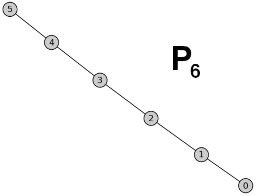
for $i,j=0,1,...,N-1$ . In particular we can choose $G_{1}$ and $G_{2}$ to be $P_{N}$ and/or $Cy_{N}$ , where $P_{N}$ is the so called path on $N$ nodes (see Figure 4.2), while $Cy_{N}$ is the cycle graph (see Figure 4.1).

Their eigenquantities (in the case of unitary weights) are:

		$\displaystyle\begin{cases}e_{P_{N}}^{i}=&2\cos\left[\frac{\left(i+1\right)\pi}{N+1}\right]\\ \\ \left[\overrightarrow{v}_{P_{N}}^{i}\right]_{j}=&\sin\left[\frac{\left(i+1\right)\left(j+1\right)\pi}{N+1}\right]\end{cases}$		(4.16)
		$\displaystyle\begin{cases}e_{Cy_{N}}^{i}=&2cos\left(\frac{2\pi i}{N}\right)\\ \\ \left[\overrightarrow{v}_{Cy_{N}}^{i}\right]_{j}=&e^{\frac{2\pi ij}{N}\iota}\end{cases},\,\iota=\sqrt{-1}$		(4.17)

Combining them through the binary operations $\otimes$ and $\times$ , we can create several classes of well-known graphs, like:

—

Ladder: $L_{n}=P_{n}\times P_{2}$ , with $2n=N$ ;
—

Circular Ladder (also known as Annulus or Prism): $CL_{n}=Cy_{n}\times P_{2}$ , with $2n=N$ ;
—

Grid: $G_{m,n}=P_{m}\times P_{n}$ , with $mn=N$ ;
—

Cylinder: $Cl_{m,n}=P_{m}\times Cy_{n}$ , with $mn=N$ ;
—

Torus: $T_{m,n}=Cy_{m}\times Cy_{n}$ , with $mn=N$ ;
—

Cross: $Cr_{m,n}=P_{m}\otimes P_{n}$ , with $mn=N$ ;
—

Hypercube: $H_{n}=\underset{n-times}{\underbrace{P_{2}\times P_{2}\times...\times P_{2}}}$ , with $2^{n}=N$ ;

and so on and so forth. Some of these examples are shown in the Figures 4.3 and 4.4. Even much more complicated graphs can be created in this way, like $Cr_{m,n}\otimes T_{p,q}$ , or $G_{m,n}\otimes T_{p,q}\times H_{r}\otimes Cl_{x,y}$ , and so on.

Using the mixed-product property of the Kronecker product, we obtain:

\overrightarrow{v}_{P_{N_{1}}\otimes P_{N_{2}}}^{i,j}\cdot\overrightarrow{v}_{P_{N_{1}}\otimes P_{N_{2}}}^{k,l}=\left(\overrightarrow{v}_{P_{N_{1}}}^{i}\cdot\overrightarrow{v}_{P_{N_{1}}}^{k}\right)\left(\overrightarrow{v}_{P_{N_{2}}}^{j}\cdot\overrightarrow{v}_{P_{N_{2}}}^{l}\right)=0

if $i\neq k$ and/or $j\neq l$ , since the eigenvectors of the path are orthogonal (of course the same is true for $\overrightarrow{v}_{P_{N_{1}}\times P_{N_{2}}}^{i,j}\cdot\overrightarrow{v}_{P_{N_{1}}\times P_{N_{2}}}^{k,l}$ ). Therefore the eigenvectors $\overrightarrow{v}_{P_{N_{1}}\otimes P_{N_{2}}}^{i,j}$ (or equivalently $\overrightarrow{v}_{P_{N_{1}}\times P_{N_{2}}}^{i,j}$ ) are orthogonal. Moreover $\overrightarrow{v}_{P_{N_{1}}\otimes P_{N_{2}}}^{i,j}$ have real entries, therefore they form an orthogonal matrix, that can be used directly to compute $\Phi\left(t\right)$ and $\Phi\left(t\right)\Phi^{T}\left(t\right)$ through formula .

For the eigenvectors $\overrightarrow{v}_{Cy_{N_{1}}\otimes Cy_{N_{2}}}^{i,j}$ the procedure is slightly more complicated, since the eigenvectors $\overrightarrow{v}_{Cy_{N}}^{i}$ have in general complex entries (with only the exception of the cases $i=0$ and $i=\frac{N}{2}$ for $N$ even) and therefore we cannot use them to form an orthogonal matrix. However, if $\overline{J}$ is the connectivity matrix corresponding to the graph $Cy_{N}$ , we have:

\overline{J}\overrightarrow{v}_{Cy_{N}}^{i}=e_{Cy_{N}}^{i}\overrightarrow{v}_{Cy_{N}}^{i}

which implies:

\overline{J}^{*}\left(\overrightarrow{v}_{Cy_{N}}^{i}\right)^{*}=\left(e_{Cy_{N}}^{i}\right)^{*}\left(\overrightarrow{v}_{Cy_{N}}^{i}\right)^{*}

where $*$ is the element-by-element complex conjugation. Since $\overline{J}$ and $e_{Cy_{N}}^{i}$ are real, we obtain that $\overrightarrow{v}_{Cy_{N}}^{i}$ and $\left(\overrightarrow{v}_{Cy_{N}}^{i}\right)^{*}$ are both eigenvectors of $\overline{J}$ , corresponding to the same eigenvalue $e_{Cy_{N}}^{i}$ . Therefore, if for all the complex eigenvectors $\overrightarrow{v}_{Cy_{N}}^{i}$ we define the new vectors:

	$\displaystyle\overrightarrow{V}_{Cy_{N}}^{i}=$	$\displaystyle\frac{1}{2}\left(\overrightarrow{v}_{Cy_{N}}^{i}+\left[\overrightarrow{v}_{Cy_{N}}^{i}\right]^{*}\right)$
	$\displaystyle\overrightarrow{W}_{Cy_{N}}^{i}=$	$\displaystyle\frac{1}{2\iota}\left(\overrightarrow{v}_{Cy_{N}}^{i}-\left[\overrightarrow{v}_{Cy_{N}}^{i}\right]^{*}\right)$

we conclude that they are eigenvectors of $\overline{J}$ with eigenvalue $e_{Cy_{N}}^{i}$ . Now, it is easy to see that $\overrightarrow{V}_{Cy_{N}}^{i}\cdot\overrightarrow{W}_{Cy_{N}}^{j}=0$ $\forall i,j$ . Moreover $\overrightarrow{V}_{Cy_{N}}^{i}$ and $\overrightarrow{W}_{Cy_{N}}^{i}$ are orthogonal also to $\overrightarrow{V}_{Cy_{N}}^{0}$ and $\overrightarrow{V}_{Cy_{N}}^{\frac{N}{2}}$ in the case of $N$ even, and their entries are real. Therefore, if we use this set of real eigenvectors with the rules 4.14 or 4.15, we obtain a set of eigenvectors for $Cy_{N_{1}}\otimes Cy_{N_{2}}$ or $Cy_{N_{1}}\times Cy_{N_{2}}$ which are orthogonal and real (the proof is similar to the case $P_{N_{1}}\otimes P_{N_{2}}$ seen before). So they can be used to form an orthogonal matrix, through which we can compute $\Phi\left(t\right)$ and $\Phi\left(t\right)\Phi^{T}\left(t\right)$ , according to formula .

To conclude, taking for example the cases we have written previously, it is important to observe that only the graphs $CL_{n}$ , $T_{m,n}$ and $H_{n}$ can be considered in our analysis. In effect these three graphs have the same number of incoming connections per neuron, a feature that is not shown by the ladder, the grid etc, due to their boundaries. The latter graphs can be studied using this approach only in the thermodynamic limit $N\rightarrow\infty$ . In fact only in this case the number of incoming connections per neuron is the same for all the neurons in the network, because when $N\rightarrow\infty$ the system "loses" its boundaries, since they are pushed to infinity. For example, in the graph $L_{n}$ all the neurons have $3$ incoming connections (see neurons $1-4$ and $7-10$ in the case of the graph $L_{6}$ shown in Figure 4.3), with only the exception of those at the boundaries, which have only $2$ connections (see neurons $0$ , $5$ , $6$ and $11$ in Figure 4.3). When $N\rightarrow\infty$ , if we start to travel on the ladder from its center toward the boundaries, we will never reach them, since they are at infinity, therefore during the trip we meet only neurons with the same number (namely $3$ ) of incoming connections. Therefore in the thermodynamic limit all the neurons of the graphs with boundaries behave in the same way. This means that we have obtained the invariance of the system under exchange of the neural indices, which is what we need in order to apply the perturbative approach introduced in this article.

5 Numerical comparison

The Figures 5.1 - 5.7 show the numerical comparison obtained with the first-order perturbative expansion. For simplicity in this case we have chosen $\sigma_{4}=\sigma_{5}=0$ , since according to 3.1 these two parameters affect the covariance only at a higher order. These figures report both the results obtained from the exact network equations 2.1 (blue lines) and from the first-order perturbative expansion (red lines), the latter being generated with the equations 2.15 - 2.18. Moreover we have shown the comparison with the analytic results for the variance, covariance and correlation generated by the formulae 3.1 - 3.6 (green lines). Instead the Figure 5.8 shows the results for the second-order perturbative expansion, obtained from the equations 2.15 - 2.26. For the sake of brevity, here we have reported only the results for the correlation, but we have not shown the comparison with its analytic formula (green lines), due to the complexity of the higher order terms of the variance and covariance. In this case we have used $\sigma_{4}=\sigma_{5}=1$ , $Z\left(t\right)=e^{-t}\overline{J}$ and $\overrightarrow{H}\left(t\right)=sin\left(2\pi t\right)\overrightarrow{1}$ , where $\overrightarrow{1}$ is the vector whose entries are all ones. For all these simulations we have used the parameters reported in Table 5.1, while the statistics have been calculated with $10,000$ Monte Carlo simulations. Moreover the equations 2.1 and 2.15 - 2.26 have been solved numerically using the Euler-Maruyama scheme, while the time-integrals involved in the formulae 3.2, 3.3 and 3.4 have been calculated with the trapezoidal rule. The integration time step is $\Delta t=0.1$ . The covariance and correlation have always been calculated between the $0$ th and the $1$ st neuron, while the potentials and the variances have been reported only for the former. The general conclusion is that for small enough values of the parameters $\sigma_{1}$ - $\sigma_{5}$ there is a very good agreement between the real network and the first-order perturbative expansion and that for higher values of these parameters the second-order expansion should be used. The match depends on the dynamics of the neurons, on the synaptic connectivity and on the network size, and in the case of the variance, covariance and correlation, it also depends on the number of Monte Carlo simulations used to evaluate the statistics.

Neuron	Input	Synaptic Weights	Sigmoid Function
$\tau=1$	$\overline{I}=0$	$\Lambda=1$	$T_{MAX}=1$
$C_{2}=0.4$	$C_{1}=0.3$	$C_{3}=0.5$	$\lambda=1$
			$V_{T}=0$

Table 5.1: Parameters used for all the numerical simulations of the Figures 5.1 - 7.1.

6 Correlation as a function of the input

From the formulae 3.2, 3.3, 3.4 and the effect of the non-linearity introduced by the sigmoid function $S\left(V\right)$ is evident. Through its slope, it generates an effective connectivity matrix $\overline{J}S^{\prime}\left(\mu\right)$ , which can be interpreted as the real connectivity matrix of the system if it were linear. Now, the stationary solution $\mu$ depends on the external input current $\overline{I}$ through the formula 2.15, therefore the effective synaptic strength and the correlation structure depend on $\overline{I}$ as well. In particular, it is interesting to observe that if $\left|\overline{I}\right|$ is very large, then $\left|\mu\right|$ is also very large, therefore $S^{\prime}\left(\mu\right)$ and the entries of the effective connectivity matrix are small. In other words, the neurons become (effectively) disconnected. An important consequence of this phenomenon is that, for $C_{1}=C_{2}=C_{3}=0$ and for large values of $\left|\overline{I}\right|$ , the neurons become independent, even if the size of the network is finite. This intuition is confirmed numerically in Figure 6.1, which has been obtained for the graph $Cy_{5}$ (which is made of $10$ neurons) simulated with the exact equations 2.1, for $\overline{I}=-5,0,5$ and $50,000$ Monte Carlo simulations. The sources of randomness have intensities $\sigma_{1}=\sigma_{2}=\sigma_{3}=0.1$ , and moreover $\sigma_{4}=\sigma_{5}=0$ , while all the remaining parameters are those of Table 5.1. As usual, the numerical scheme is the Euler-Maruyama one, with integration time step $\Delta t=0.1$ .

7 Failure of the mean-field theory

In this section we show three different reasons that invalidate the use of the mean-field theory for the mathematical analysis of a neural network. A neural network is generally described by a large set of stochastic differential equations, that makes it hard to understand the underlying behavior of the system. However, if the neurons become independent, their dynamics can be described with the mean-field theory using a highly reduced set of equations, that are much simpler to analyze. For this reason the mean-field theory is a powerful tool that can be used to understand the network. One of the mechanisms through which the independence of the neurons can be obtained is the phenomenon known as propagation of chaos [9][23][24][25]. Propagation of chaos refers to the fact that, if we choose independent initial conditions for the membrane potentials at $t=0$ (which may be called initial chaos), then the neurons are always perfectly independent $\forall t>0$ . Therefore the term propagation refers to the “transfer” of the independence of the membrane potentials from $t=0$ to $t>0$ . Under simplified assumptions about the nature of the network (namely that the other sources of randomness in the system, in our case the Brownian motions and the synaptic weights, are independent), propagation of chaos does occur in the so called thermodynamic limit of the system, namely when the number of neurons in the system grows to infinity. However in Sections 7.1, 7.2 and 7.3 we show that for a system with correlated Brownian motions, initial conditions and synaptic weights, with a general connectivity matrix or with an arbitrarily large (but still finite) size, the correlation between pairs of neurons can be high. Therefore in general the neurons cannot be independent, invalidating the use of the mean-field theory.

7.1 Independence does not occur for $N\rightarrow\infty$ if $C_{1}$ , $C_{2}$ or $C_{3}$ are not equal to zero

Let us consider the case when at least one of the parameters $C_{1}$ , $C_{2}$ and $C_{3}$ (defined by , 2 and 2.12) is not equal to zero. For example we analyze the term proportional to $C_{1}$ in the formula 3.2, for a fully connected network. Using the technique developed in Section 4.1, it is easy to prove that this term for $i\neq j$ is:

		$\displaystyle C_{1}{\displaystyle\sum\limits_{\begin{subarray}{c}k,l=0\\ k\neq l\end{subarray}}^{N-1}}\int_{0}^{t}\left[\Phi\left(t-s\right)\right]_{ik}\left[\Phi\left(t-s\right)\right]_{jl}ds$
		$\displaystyle=\frac{C_{1}}{2}\left\{\left(1-\frac{1}{N}\right)\frac{1}{\frac{1}{\tau}-\Lambda S^{\prime}\left(\mu\right)}\left[1-e^{-2\left(\frac{1}{\tau}-\Lambda S^{\prime}\left(\mu\right)\right)t}\right]+\frac{1}{N}\frac{1}{\frac{1}{\tau}+\frac{\Lambda S^{\prime}\left(\mu\right)}{N-1}}\left[1-e^{-2\left(\frac{1}{\tau}+\frac{\Lambda S^{\prime}\left(\mu\right)}{N-1}\right)t}\right]\right\}$

while for $i=j$ it is:

		$\displaystyle C_{1}{\displaystyle\sum\limits_{\begin{subarray}{c}k,l=0\\ k\neq l\end{subarray}}^{N-1}}\int_{0}^{t}\left[\Phi\left(t-s\right)\right]_{ik}\left[\Phi\left(t-s\right)\right]_{il}ds$
		$\displaystyle=\frac{C_{1}}{2}\left(1-\frac{1}{N}\right)\left\{\frac{1}{\frac{1}{\tau}-\Lambda S^{\prime}\left(\mu\right)}\left[1-e^{-2\left(\frac{1}{\tau}-\Lambda S^{\prime}\left(\mu\right)\right)t}\right]-\frac{1}{\frac{1}{\tau}+\frac{\Lambda S^{\prime}\left(\mu\right)}{N-1}}\left[1-e^{-2\left(\frac{1}{\tau}+\frac{\Lambda S^{\prime}\left(\mu\right)}{N-1}\right)t}\right]\right\}$

So the covariance (and therefore also the correlation) does not go to zero for $N\rightarrow\infty$ , or in other words the neurons are not independent, even in the thermodynamic limit.

The reader can easily check that the same result holds for the terms of the covariance proportional to $C_{2}$ and $C_{3}$ .

7.2 Propagation of chaos does not occur for a general connectivity matrix

We study propagation of chaos as a function of the number of connections in the circulant network. To this purpose, we have to set $C_{2}=0$ (initial chaos) and also $C_{1}=C_{3}=0$ , because otherwise the neurons cannot be independent, as explained in Section 7.1. Using the formulae 3.2, 3.3, 3.4 and we obtain that in this case the covariance is:

	$\displaystyle Cov\left(V_{i}\left(t\right),V_{j}\left(t\right)\right)=$	$\displaystyle\sigma_{1}^{2}\int_{0}^{t}\left[\Phi\left(t-s\right)\Phi^{T}\left(t-s\right)\right]_{ij}ds+\sigma_{2}^{2}\left[\Phi\left(t\right)\Phi^{T}\left(t\right)\right]_{ij}$
		$\displaystyle+\sigma_{3}^{2}\frac{S^{2}\left(\mu\right)}{M}\sum_{k=0}^{N-1}\left[\int_{0}^{t}\Phi_{ik}\left(t-s\right)ds\right]\left[\int_{0}^{t}\Phi_{jk}\left(t-s\right)ds\right]$		(7.1)

where:

		$\displaystyle\int_{0}^{t}\left[\Phi\left(t-s\right)\Phi^{T}\left(t-s\right)\right]_{ij}ds=\frac{1}{2N}\sum_{k=0}^{N-1}\frac{cos\left[\frac{2\pi}{N}k\left(i-j\right)\right]}{-\frac{1}{\tau}+e_{k}S^{\prime}\left(\mu\right)}\left\{1-e^{2\left[-\frac{1}{\tau}+S^{\prime}\left(\mu\right)e_{k}\right]t}\right\}$
		$\displaystyle\left[\Phi\left(t\right)\Phi^{T}\left(t\right)\right]_{ij}=\frac{1}{N}\sum_{k=0}^{N-1}e^{2\left[-\frac{1}{\tau}+S^{\prime}\left(\mu\right)e_{k}\right]t}cos\left[\frac{2\pi}{N}k\left(i-j\right)\right]$
		$\displaystyle\sum_{k=0}^{N-1}\left[\int_{0}^{t}\Phi_{ik}\left(t-s\right)ds\right]\left[\int_{0}^{t}\Phi_{jk}\left(t-s\right)ds\right]$
		$\displaystyle=\frac{1}{N^{2}}\sum_{l,m=0}^{N-1}e^{\frac{2\pi}{N}li\iota}e^{\frac{2\pi}{N}mj\iota}\left[\sum_{k=0}^{N-1}e^{-\frac{2\pi}{N}\left(l+m\right)k\iota}\right]\left\{\frac{1-e^{\left[-\frac{1}{\tau}+S^{\prime}\left(\mu\right)e_{l}\right]t}}{-\frac{1}{\tau}+e_{l}S^{\prime}\left(\mu\right)}\right\}\left\{\frac{1-e^{\left[-\frac{1}{\tau}+S^{\prime}\left(\mu\right)e_{m}\right]t}}{-\frac{1}{\tau}+e_{m}S^{\prime}\left(\mu\right)}\right\}$
		$\displaystyle=\frac{1}{N}\sum_{l=0}^{N-1}\left\{\frac{1-e^{\left[-\frac{1}{\tau}+S^{\prime}\left(\mu\right)e_{l}\right]t}}{-\frac{1}{\tau}+e_{l}S^{\prime}\left(\mu\right)}\right\}^{2}cos\left[\frac{2\pi}{N}l\left(i-j\right)\right]$

while the eigenvalues $e_{k}$ are given by formula 4.11 or by formula 4.12. Now, for $N\rightarrow\infty$ the right-hand side of formula 7.1 converges to a non-zero function (see Figure 7.1), therefore for every finite value of $\nu$ (which is the number of incoming connections per neuron divided by $2$ ) propagation of chaos does not occur.

Moreover correlation decreases with $\nu$ , therefore propagation of chaos occurs in the circulant network only in the thermodynamic limit $N\rightarrow\infty$ and if $\nu$ is an increasing function of $N$ , namely if $\underset{N\rightarrow\infty}{lim}\nu=\infty$ . For example, in the fully connected network $\nu=\left\lfloor\frac{N}{2}\right\rfloor$ , so it explains why in this case correlation goes to zero in the thermodynamic limit. Instead in a network described by a cycle graph, perfect decorrelation is never possible, also for $N\rightarrow\infty$ , since $\nu=1$ . In other words, having infinitely many neurons is not a sufficient condition for getting propagation of chaos, because also infinite connections per neuron are required.

7.3 Stochastic synchronization

In this section we show that for every finite and arbitrarily large number of neurons $N$ in the network, it is possible to choose special values of the parameters of the system such that, at some finite and arbitrarily large time instant $\overline{t}$ , the correlation between pairs of neurons is (approximately) $1$ . In general $\overline{t}$ increases with $N$ .

7.3.1 The general theory

We show that even when $C_{1}=C_{2}=C_{3}=0$ , if the matrix $A=-\frac{1}{\tau}Id_{N}+\overline{J}S^{\prime}\left(\mu\right)$ has an eigenvalue of multiplicity $1$ with non-negative real part, while all the other eigenvalues have negative real parts, then correlation goes to $1$ for $t\rightarrow+\infty$ , for every finite $N$ . In other terms, the stochastic components of the membrane potentials become perfectly synchronized. From now on we refer to this phenomenon as stochastic synchronization. To prove this, we suppose that $A$ has an eigenvalue $\overline{a}$ with non-negative real part and with a generic multiplicity $m>0$ , while all the other eigenvalues have negative real parts. Now we recall that $e^{At}=Qe^{Dt}Q^{-1}$ , where $D$ is the diagonal matrix of the eigenvalues of $A$ , and $Q$ is the matrix of its eigenvectors. So for $t\rightarrow+\infty$ we have:

e^{Dt}\prec diag(0,0,...,0,\underset{m\mathrm{-times}}{\underbrace{e^{\overline{a}t},e^{\overline{a}t},...,e^{\overline{a}t}}},0,0,...,0)

where $\prec$ means dominated by, because all the eigenvalues have negative real part but $\overline{a}$ . If the $\overline{a}$ s are the $r$ -th, $\left(r+1\right)$ -th, …, $\left(r+m-1\right)$ -th eigenvalues of $A$ and if we call $Q^{-1}=B$ in order to simplify the notation, we obtain:

	$\displaystyle Qe^{Dt}B\prec$	$\displaystyle e^{\overline{a}t}\left[\begin{array}[]{cccccccccccc}0&0&\cdots&0&Q_{0,r}&Q_{0,r+1}&\cdots&Q_{0,r+m-1}&0&0&\cdots&0\\ 0&0&\cdots&0&Q_{1,r}&Q_{1,r+1}&\cdots&Q_{1,r+m-1}&0&0&\cdots&0\\ \vdots&\vdots&\ddots&\vdots&\vdots&\vdots&\ddots&\vdots&\vdots&\vdots&\ddots&\vdots\\ 0&0&\cdots&0&Q_{N-1,r}&Q_{N-1,r+1}&\cdots&Q_{N-1,r+m-1}&0&0&\cdots&0\end{array}\right]$
		$\displaystyle\times\left[\begin{array}[]{cccc}B_{0,0}&B_{0,1}&...&B_{0,N-1}\\ B_{1,0}&B_{1,1}&...&B_{1,N-1}\\ \vdots&\vdots&\ddots&\vdots\\ B_{N-1,0}&B_{N-1,1}&...&B_{N-1,N-1}\end{array}\right]$

and therefore:

	$\displaystyle e^{At}=$	$\displaystyle Qe^{Dt}B\prec e^{\overline{a}t}E$
	$\displaystyle E_{pq}=$	$\displaystyle\sum_{k=0}^{m-1}Q_{p,r+k}B_{r+k,q}$

This means that:

$\displaystyle Cov\left(V_{i}\left(t\right),V_{j}\left(t\right)\right)=$	$\displaystyle\sigma_{1}^{2}{\displaystyle\sum_{k=0}^{N-1}}\int_{0}^{t}\left[e^{A\left(t-s\right)}\right]_{ik}\left[e^{A\left(t-s\right)}\right]_{jk}ds+\sigma_{2}^{2}{\displaystyle\sum_{k=0}^{N-1}}\left[e^{At}\right]_{ik}\left[e^{At}\right]_{jk}$
	$\displaystyle+\sigma_{3}^{2}\frac{S^{2}\left(\mu\right)}{M}{\displaystyle\sum_{k=0}^{N-1}}\left\{\int_{0}^{t}\left[e^{A\left(t-s\right)}\right]_{ik}ds\right\}\left\{\int_{0}^{t}\left[e^{A\left(t-s\right)}\right]_{jk}ds\right\}$
$\displaystyle\prec$	$\displaystyle\left[\frac{\sigma_{1}^{2}}{2\overline{a}}+\sigma_{2}^{2}+\frac{\sigma_{3}^{2}}{\overline{a}^{2}}\frac{S^{2}\left(\mu\right)}{M}\right]e^{2\overline{a}t}{\displaystyle\sum_{k=0}^{N-1}}E_{ik}E_{jk}$	(7.2)

so the variance is:

Var\left(V_{i}\left(t\right)\right)=Cov\left(V_{i}\left(t\right),V_{i}\left(t\right)\right)\prec\left[\frac{\sigma_{1}^{2}}{2\overline{a}}+\sigma_{2}^{2}+\frac{\sigma_{3}^{2}}{\overline{a}^{2}}\frac{S^{2}\left(\mu\right)}{M}\right]e^{2\overline{a}t}\sum_{k=0}^{N-1}\left(E_{ik}\right)^{2}

(7.3)

Therefore the correlation is:

Corr\left(V_{i}\left(t\right),V_{j}\left(t\right)\right)=\frac{Cov\left(V_{i}\left(t\right),V_{j}\left(t\right)\right)}{\sqrt{Var\left(V_{i}\left(t\right)\right)Var\left(V_{j}\left(t\right)\right)}}\rightarrow\frac{{\displaystyle\sum_{k=0}^{N-1}}E_{ik}E_{jk}}{\sqrt{\left[{\displaystyle\sum_{k=0}^{N-1}}\left(E_{ik}\right)^{2}\right]\left[{\displaystyle\sum_{k=0}^{N-1}}\left(E_{jk}\right)^{2}\right]}}

(7.4)

when $t\rightarrow+\infty$ . Now, in the special case $m=1$ we obtain:

	$\displaystyle E_{pq}=$	$\displaystyle Q_{pr}B_{rq}$
	$\displaystyle\sum_{k=0}^{N-1}E_{ik}E_{jk}=$	$\displaystyle Q_{ir}Q_{jr}\sum_{k=0}^{N-1}\left(B_{rk}\right)^{2}$
	$\displaystyle\sum_{k=0}^{N-1}\left(E_{ik}\right)^{2}=$	$\displaystyle\left(Q_{ir}\right)^{2}\sum_{k=0}^{N-1}\left(B_{rk}\right)^{2}$

so we conclude that $Corr\left(V_{i}\left(t\right),V_{j}\left(t\right)\right)\rightarrow 1$ when $t\rightarrow+\infty$ . This proves that if $C_{1}=C_{2}=C_{3}=0$ and the matrix $A$ has an eigenvalue of multiplicity $1$ with non-negative real part while all the other eigenvalues have negative real parts, then propagation of chaos does not occur. For continuity, for every finite $N$ we have that $Corr\left(V_{i}\left(t\right),V_{j}\left(t\right)\right)\rightarrow 1$ also for $\mathcal{R}\left(\overline{a}\right)\rightarrow 0^{-}$ (where $\mathcal{R}$ means the real part of), i.e. correlation is very big also when the system is stable but close to the instability region $\mathcal{R}\left(\overline{a}\right)>0$ . It is also interesting to observe that, due to the Perron-Frobenius theorem [33], if $\Lambda>0$ and if $\overline{J}$ is an irreducible matrix (namely if its corresponding directed graph is strongly connected, which means that it is possible to reach each vertex in the graph from any other vertex, by moving on the edges according to their connectivity directions), then it has a unique largest positive eigenvalue, which can be used to generate stochastic synchronization. We conclude that in general propagation of chaos does not always occur, even if $C_{1}=C_{2}=C_{3}=0$ , therefore this invalidates the use of the mean-field theory, at least in this special case.

7.3.2 The example of the fully connected network

We show how to set the parameters of the system such that the phenomenon of stochastic synchronization does occur. For simplicity we assume a fully connected network. In this case, from formula 4.12, we know that the matrix $A$ has eigenvalues:

\begin{array}[]{ccc}a_{0}=-\frac{1}{\tau}+\Lambda S^{\prime}\left(\mu\right),&&a_{1}=-\frac{1}{\tau}-\frac{\Lambda S^{\prime}\left(\mu\right)}{N-1}\end{array}

(7.5)

The multiplicity of $a_{0}$ and $a_{1}$ is respectively $1$ and $N-1$ , therefore in order to obtain the stochastic synchronization, according to Section 7.3.1, we have to set $a_{0}\geq 0$ . Let us consider the case $a_{0}=0$ , namely $\Lambda S^{\prime}\left(\mu\right)=\frac{1}{\tau}$ . Now, since:

S^{\prime}\left(\mu\right)=\lambda\left[S\left(\mu\right)-\frac{S^{2}\left(\mu\right)}{T_{MAX}}\right]

(7.6)

we obtain the algebraic equation:

\Lambda\lambda\left[S\left(\mu\right)-\frac{S^{2}\left(\mu\right)}{T_{MAX}}\right]=\frac{1}{\tau}

whose solutions are:

S\left(\mu_{1,2}\right)=T_{MAX}\frac{1\pm\sqrt{1-\frac{4}{\tau\Lambda\lambda T_{MAX}}}}{2}

(7.7)

where $\mu_{1,2}$ are two possible stationary solutions of the membrane potential. Moreover, from equation 2.15 we know that:

\mu_{1,2}=\tau\left[\Lambda S\left(\mu_{1,2}\right)+\overline{I}\right]

(7.8)

Putting together the formulae 7.7 and 7.8 we obtain:

\mu_{1,2}=\tau\left(\Lambda T_{MAX}\frac{1\pm\sqrt{1-\frac{4}{\tau\Lambda\lambda T_{MAX}}}}{2}+\overline{I}\right)

(7.9)

Replace this value of $\mu_{1,2}$ in 7.8 to obtain the final result:

T_{MAX}\frac{1\pm\sqrt{1-\frac{4}{\tau\Lambda\lambda T_{MAX}}}}{2}=S\left(\tau\left(\Lambda T_{MAX}\frac{1\pm\sqrt{1-\frac{4}{\tau\Lambda\lambda T_{MAX}}}}{2}+\overline{I}\right)\right)

(7.10)

This non-linear algebraic equation is the constraint that must be satisfied by all the parameters of the system in order to have correlation equal to $1$ in the limit $t\rightarrow+\infty$ . An example of solution of this equation is $\lambda=T_{MAX}=1$ , $V_{T}=0$ , $\Lambda=-2\overline{I}$ and $\tau=-\frac{2}{\overline{I}}$ , $\forall\overline{I}<0$ . In this case $\mu_{1,2}=0$ and it can be used as initial condition in order to ensure the stationarity of the system. In Figure 7.2 we show the phenomenon of stochastic synchronization in the case of a fully connected network, for the values of the parameters reported in Table 7.1, which satisfy the constraint 7.10. As we can see, correlation goes to $1$ more and more slowly if we increase the number of neurons $N$ in the network. It reaches the value $1$ asymptotically with an inverse exponential-like behavior, with a time constant that increases with the size of the network. For $N\rightarrow\infty$ the time constant diverges, therefore for every finite time the system has correlation $0$ . This proves that in the thermodynamic limit there is still propagation of chaos, provided that $C_{1}=C_{2}=C_{3}=0$ . This is in perfect agreement with the result on propagation of chaos proved in [9][23][25] for independent Brownian motions, initial conditions and synaptic weights.

Neuron	Input	Synaptic Weights	Sigmoid Function
$\tau=0.1$	$\overline{I}=-20$	$\Lambda=40$	$T_{MAX}=1$
$C_{2}=0$	$C_{1}=0$	$C_{3}=0$	$\lambda=1$
			$V_{T}=0$

Table 7.1: Parameters used for the numerical simulations of Figure 7.2.

8 Conclusion

In this work we have developed a perturbative expansion that let us determine the dynamics and the correlation structure of a neural network made up of a finite number of rate neurons and with specific connectivity matrices.

The network has three independent sources of randomness in the stochastic fluctuations of the membrane potentials (or in the external input current), in the initial conditions and in the synaptic weights.

Their probability distributions are supposed to be normal with known correlation matrices, moreover we have assumed that the system is invariant under exchange of the neural indices, without any other assumption on the intensity of the synaptic weights.

This has allowed us to obtain analytic results, even if the equations of the network are non-linear, which have been confirmed numerically.

With this approach we have analyzed block circulant and special symmetric connections obtained from the composition of circulant and path graphs.

In the former case, when the correlations of the noise, the initial conditions and the synaptic weights are set to zero, we have proved that propagation of chaos of the membrane potentials increases with the number of incoming connections per neuron in the network, and not with the number of neurons, as previously thought.

Instead, if the correlations of the three sources of randomness are not set to zero, propagation of chaos in general does not occur, even if the number of connections per neuron in the network is infinite.

Moreover, for special values of the parameters of the system, we have proved that the membrane potentials become perfectly correlated, a phenomenon that we have called stochastic synchronization.

This phenomenon occurs, for any finite number of neurons, even if the correlations of the three sources of randomness are set to zero.

In this case the correlation of the membrane potentials starts to increase from zero and it reaches the value $1$ (namely perfect correlation) at a time instant that increases with the number of neurons in the network.

Therefore for an infinite number of neurons, i.e. in the mean-field limit of the system, correlation is always equal to zero for any finite time instant.

This is in agreement with the results proved in [9][23][25].

Moreover, we have shown how to use these perturbative expansions in the calculation of higher order correlations, like those between triplets, quadruplets, quintuplets etc of neurons.

So with this approach we can determine all the moments of the joint probability density, but in general we are not able to evaluate the probability density itself.

In principle the moments can be used to calculate the moment-generating function, from whom we could determine the corresponding probability density, but in practice this is not feasible.

So we only know that at the first perturbative order the process is normal, while at the second order it is a generalized chi-squared process.

The generalized chi-squared process can be defined as the sum of products between pairs of normal processes, but its probability density is not known, since it is still an open problem.

The same issue persists at higher orders, so another approach must be followed.

Since the probability density is usually described by the Fokker-Planck equation, we could think to solve it perturbatively.

However for a network with finite size we cannot use the trick of the mean-field dimensional reduction, since here we have proved that propagation of chaos does not occur, therefore the corresponding Fokker-Planck equation would be high-dimensional.

Another problem with this approach is the second order derivative of the equation, that describes the diffusion process.

This term is multiplied by the intensity of the Brownian motions $\sigma_{1}$ , forcing us to use the singular perturbation theory.

So this idea is not promising, leaving the problem open.

Even if we have developed this perturbative expansion for a rate model with generic evolutions of the synaptic weights, we can apply them to other kinds of models.

For example, we can consider spiking networks, described for example by the FitzHugh-Nagumo or the Hodgkin-Huxley model.

In this case the perturbative expansion is useful only for the description of the sub-threshold activity, since over the threshold the neurons are spiking and so there is no stationary solution around which the membrane potential can be expanded.

This is a different situation compared to the rate model, since in this latter case also a stationary solution $\mu$ describes a spiking activity, with rate $S\left(\mu\right)$ .

To conclude, we have proved that the perturbative method developed in this article sheds new light in the comprehension of stochastic neural networks, with special emphasis on finite size effects and correlation.

In particular, these results establish the relation between the functional and anatomical connectivity of the network, a problem that is currently intensively investigated.

Moreover, at the first perturbative order, the probability density of the system is a multivariate normal distribution.

For such a probability density, the information quanties like the Shannon information, the Fisher information and the transfer entropy [34], can be evaluated analytically for any finite number of neurons.

This is a big advantage since otherwise these quantities can be evaluated only through the calculation of high-dimensional integrals using the Monte Carlo integration.

Therefore this allows us to quantify the information processing capabilities of the neural networks, in terms of information encoding, storage, transmission and modification, following the same ideas already developed in the field of automata theory [35][36][37][38].

We think now we are in a much better position for understanding in detail the working principles of stochastic neural networks.

Appendix A Radius of convergence of the sigmoid and arctangent functions

In this section we compute numerically the radius of convergence of two examples of the activation function $S\left(\cdot\right)$ . For simplicity we consider only the case with $T_{MAX}=1$ and $V_{T}=0$ , but this analysis can be extended easily to the most general case.

A.1 The sigmoid function

According to [39], the $n$ -th order derivative of the sigmoid function:

S\left(x\right)=\frac{1}{1+e^{-\lambda x}}

is:

S^{\left(n\right)}\left(x\right)=\lambda^{n}\sum_{k=1}^{n}\left(-1\right)^{k-1}A\left(n,k-1\right)\left[S\left(x\right)\right]^{k}\left[1-S\left(x\right)\right]^{n+1-k}

where $A\left(n,k\right)$ are the so called Eulerian numbers [40]. Now we can rewrite this expression in the following way:

	$\displaystyle S^{\left(n\right)}\left(x\right)=$	$\displaystyle\lambda^{n}S\left(x\right)\left[1-S\left(x\right)\right]^{n}\sum_{k=1}^{n}\left(-1\right)^{k-1}A\left(n,k-1\right)\left[S\left(x\right)\right]^{k-1}\left[1-S\left(x\right)\right]^{-\left(k-1\right)}$
	$\displaystyle=$	$\displaystyle\lambda^{n}S\left(x\right)\left[1-S\left(x\right)\right]^{n}\sum_{k=0}^{n-1}\left(-1\right)^{k}A\left(n,k\right)\left[S\left(x\right)\right]^{k}\left[1-S\left(x\right)\right]^{-k}$
	$\displaystyle=$	$\displaystyle\lambda^{n}S\left(x\right)\left[1-S\left(x\right)\right]^{n}\sum_{k=0}^{n-1}A\left(n,k\right)\left(-e^{-\lambda x}\right)^{-k}$

Now from [41], we know that:

\begin{array}[]{ccc}Li_{-n}\left(x\right)=\frac{x^{n}}{\left(1-x\right)^{n+1}}{\displaystyle\sum_{k=0}^{n-1}}A\left(n,k\right)x^{-k},&&n>0,\>\left|x\right|<1\end{array}

(A.1)

where $Li_{-n}\left(\cdot\right)$ represents the so called polylogarithm (with negative order). Here we have omitted the $n$ -th term of the sum since $A\left(n,n\right)=0$ $\forall n>0$ . So we can write:

S^{\left(n\right)}\left(x\right)=\lambda^{n}S\left(x\right)\left[1-S\left(x\right)\right]^{n}\frac{\left(1+e^{-\lambda x}\right)^{n+1}}{\left(-e^{-\lambda x}\right)^{n}}Li_{-n}\left(-e^{-\lambda x}\right)=\left(-\lambda\right)^{n}Li_{-n}\left(-e^{-\lambda x}\right)

(A.2)

This result is true only for $\left|-e^{-\lambda x}\right|<1$ , i.e. only for $x>0$ . Instead, for $x<0$ , we can use the relation $S\left(-x\right)=1-S\left(x\right)$ , from which we deduce that:

—

$S^{\left(n\right)}\left(-x\right)=\left(-1\right)^{n-1}S^{\left(n\right)}\left(x\right),$ $\forall n>0$ ;
—

$S\left(-x\right)$ has the same radius of convergence of $S\left(x\right)$ .

So formula A.2 can be used to express $S^{\left(n\right)}\left(x\right)$ $\forall x\neq 0$ . Instead for $x=0$ it gives $Li_{-n}\left(-1\right)$ , that is defined by an analytic continuation of the polylogarithm function. In this way we can determine $S^{\left(n\right)}\left(0\right)$ . Another way is to use the following property of the Eulerian numbers:

\sum_{k=1}^{n}\left(-1\right)^{k-1}A\left(n,k-1\right)=2^{n+1}\left(2^{n+1}-1\right)\frac{B_{n+1}}{n+1}

(A.3)

where $B_{n}$ are the so called Bernoulli numbers [42], from which we obtain:

S^{\left(n\right)}\left(0\right)=\frac{\lambda^{n}}{2^{n+1}}\sum_{k=1}^{n}\left(-1\right)^{k-1}A\left(n,k-1\right)=\lambda^{n}\left(2^{n+1}-1\right)\frac{B_{n+1}}{n+1}

(A.4)

Now we can compute the radius of convergence $R\left(x_{0}\right)$ of the Taylor series:

S\left(x\right)=\sum_{n=0}^{+\infty}\frac{S^{\left(n\right)}\left(x_{0}\right)}{n!}\left(x-x_{0}\right)^{n}

using the Cauchy root test:

R\left(x_{0}\right)=\frac{1}{\underset{n\rightarrow+\infty}{lim\,sup}\sqrt[n]{\left|\frac{S^{\left(n\right)}\left(x_{0}\right)}{n!}\right|}}

For $x_{0}=0$ we obtain:

R\left(0\right)=\frac{1}{\underset{n\rightarrow+\infty}{lim\,sup}\sqrt[n]{\left|\frac{\lambda^{n}\left(2^{n+1}-1\right)\frac{B_{n+1}}{n+1}}{n!}\right|}}=\frac{\pi}{\lambda}

This can be proved after the substitution $n\rightarrow 2n-1$ (which is motivated by the fact that $B_{2n+1}=0$ $\forall n>0$ ), using the following asymptotic expansion of the Bernoulli numbers:

\begin{array}[]{ccc}B_{2n}\sim\left(-1\right)^{n-1}4\sqrt{\pi n}\left(\frac{n}{\pi e}\right)^{2n},&&n\rightarrow+\infty\end{array}

and the Stirling approximation of $\left(2n-1\right)!$ . We are not aware of any asymptotic expansion of $Li_{-n}\left(-e^{-x_{0}}\right)$ for $n\rightarrow+\infty$ and $x_{0}\neq 0$ , so we have to compute the radius of convergence numerically $\forall x_{0}\neq 0$ .

Figure A.1 shows the result for different values of $\lambda$ . From it we can see that the radius of convergence of the Taylor series of $S\left(x\right)$ around the point $x=x_{0}$ increases with $x_{0}$ . This is reasonable, since the function $S\left(x\right)$ becomes flat when $x$ is large. Moreover for large $\lambda$ it converges to $R\left(x_{0}\right)=\left|x_{0}\right|$ and therefore it is equal to zero only for $x_{0}=0$ , as it must be. In fact, for $\lambda\rightarrow+\infty$ the function $S\left(x\right)$ converges to the Heaviside step function, which has a vertical jump at $x=0$ .

A.2 The arctangent function

Now we calculate the radius of convergence of the arctangent function. According to [43], the $n$ -th order derivative of this function is:

arctan^{\left(n\right)}\left(\lambda x\right)=\lambda^{n}\frac{\left(-1\right)^{n-1}\left(n-1\right)!}{\left[1+\left(\lambda x\right)^{2}\right]^{\frac{n}{2}}}\sin\left[n\arcsin\left(\frac{1}{\sqrt{1+\left(\lambda x\right)^{2}}}\right)\right]

So from the root test we obtain:

R\left(x_{0}\right)=\frac{\sqrt{1+\left(\lambda x_{0}\right)^{2}}}{\lambda\underset{n\rightarrow+\infty}{lim\>sup}\frac{\sqrt[n]{\left|\sin\left[n\arcsin\left(\frac{1}{\sqrt{1+\left(\lambda x_{0}\right)^{2}}}\right)\right]\right|}}{\sqrt[n]{n}}}

Now, since:

\underset{n\rightarrow+\infty}{lim}\sqrt[n]{\left|\sin\left(n\arcsin\left(\frac{1}{\sqrt{1+\left(\lambda x_{0}\right)^{2}}}\right)\right)\right|}=1

due to the fact that:

\left|\sin\left[n\arcsin\left(\frac{1}{\sqrt{1+\left(\lambda x_{0}\right)^{2}}}\right)\right]\right|\in\left[0,1\right]

and moreover $\underset{n\rightarrow+\infty}{lim}\sqrt[n]{n}=1$ , we obtain finally:

R\left(x_{0}\right)=\frac{1}{\lambda}\sqrt{1+\left(\lambda x_{0}\right)^{2}}

Therefore the radius of convergence increases with $x_{0}$ , as it must be. Moreover in the limit $\lambda\rightarrow+\infty$ it gives $R\left(x_{0}\right)=\left|x_{0}\right|$ , as with the sigmoid function.

Appendix B Higher order correlations for a fully connected neural network

Here we show how it is possible to use the perturbative expansion to calculate the higher order correlations between the neurons. For simplicity, we consider only the simplest case, namely a fully connected network, even if this analysis could be extended to more complicated connectivity matrices. Moreover we want to avoid long expressions for the joint cumulants, therefore we consider only the expansion of the membrane potential at the first perturbative order. In principle this calculation can be performed at any perturbative order, but starting from the second order (namely from the third order terms in the covariance) the functions $Z\left(t\right)$ and $\overrightarrow{H}\left(t\right)$ in general introduce inhomogeneities in the covariance structure of the network, therefore the higher order correlations should be calculated using combinatorial techniques applied to the Isserlis’ theorem. In this section we avoid the issue and we focus only on the first order perturbations. In this case the probability density of every $V_{i}\left(t\right)$ is normal and this is true also for the quantities $V_{i}\left(t\right)-\overline{V}_{i}\left(t\right)$ , which have all zero mean and the same variance, that we call $Var\left(V\left(t\right)\right)$ . Since they have zero mean we can use the Isserlis’ theorem, that for a fully connected network gives simply:

\mathbb{E}\left[\prod_{j=0}^{n-1}\left(V_{i_{j}}\left(t\right)-\overline{V}_{i_{j}}\left(t\right)\right)\right]=\begin{cases}0,&\begin{array}[]{cc}&n\mathrm{\;odd}\end{array}\\ \\ \frac{n!}{2^{\frac{n}{2}}\left(\frac{n}{2}\right)!}\left[Cov\left(V_{i}\left(t\right),V_{j}\left(t\right)\right)\right]^{\frac{n}{2}},&\begin{array}[]{cc}&n\mathrm{\;even}\end{array}\end{cases}

(B.1)

because in this case all the pairs of neurons are equivalent, since they are all-to-all connected (instead, if the network is not fully connected, the connected pairs give a different contribution with the Isserlis’ theorem compared to the disconnected pairs). Moreover, the central absolute moments of a normal distribution are:

\mathbb{E}\left[\left|V_{i_{j}}\left(t\right)-\overline{V}_{i_{j}}\left(t\right)\right|^{n}\right]=\frac{2^{\frac{n}{2}}\Gamma\left(\frac{n+1}{2}\right)}{\sqrt{\pi}}\left[Var\left(V\left(t\right)\right)\right]^{\frac{n}{2}}

(B.2)

and if $n$ is even we have $\Gamma\left(\frac{n+1}{2}\right)=\frac{n!}{2^{n}\left(\frac{n}{2}\right)!}\sqrt{\pi}$ . Therefore putting everything together we obtain:

Corr_{n}\left(V_{i_{0}}\left(t\right),V_{i_{1}}\left(t\right),...,V_{i_{n-1}}\left(t\right)\right)=\begin{cases}0,&\begin{array}[]{cc}&n\mathrm{\;odd}\end{array}\\ \\ \left[Corr_{2}\left(V_{i}\left(t\right),V_{j}\left(t\right)\right)\right]^{\frac{n}{2}},&\begin{array}[]{cc}&n\mathrm{\;even}\end{array}\end{cases}

(B.3)

From this result it is interesting to observe that if there is a perfect stochastic synchronization between pairs of neurons, then it is “propagated” to all the higher order correlations with even order, namely $Corr_{2}\left(V_{i}\left(t\right),V_{j}\left(t\right)\right)=1$ implies $Corr_{n}\left(V_{i_{0}}\left(t\right),V_{i_{1}}\left(t\right),...,V_{i_{n-1}}\left(t\right)\right)=1$ , $\forall n$ even. It is also curious to observe that all the odd order correlations are always equal to zero, even if the size of the network is finite.

Appendix C Proof that formula 4.6 gives real functions

In this appendix we want to prove that the quantities $\Phi_{ij}\left(t\right)$ and $\left[\Phi\left(t\right)\Phi^{T}\left(t\right)\right]_{ij}$ , given by formula , are real functions. The proof can be divided into four cases, namely when $R$ and $S$ are both even, both odd, $R$ even and $S$ odd, or vice versa. Here we analyze only the first case, while the others can be proved in a similar way.

So, if $R$ and $S$ are both even, the function $\Phi_{ij}\left(t\right)$ , according to , can be equivalently rewritten as:

\Phi_{ij}\left(t\right)={\displaystyle\sum_{x=0}^{R-1}}{\displaystyle\sum_{y=0}^{S-1}}e^{\left[-\frac{1}{\tau}+e_{xS+y}S^{\prime}\left(\mu\right)\right]t}f_{i,j,xS+y}

(C.1)

where now the subscripts are separated by commas, in order to avoid confusion. Defining:

g_{x,y}^{ij}=e^{\left[-\frac{1}{\tau}+e_{xS+y}S^{\prime}\left(\mu\right)\right]t}f_{i,j,xS+y}

formula C.1 can be rewritten in the following symmetric way, with respect to $R$ and $S$ :

$\displaystyle\Phi_{ij}\left(t\right)=$	$\displaystyle g_{0,0}^{ij}+g_{\frac{R}{2},0}^{ij}+g_{0,\frac{S}{2}}^{ij}+g_{\frac{R}{2},\frac{S}{2}}^{ij}$
	$\displaystyle+{\displaystyle\sum_{x=1}^{\frac{R}{2}-1}}\left[g_{x,0}^{ij}+g_{R-x,0}^{ij}\right]+{\displaystyle\sum_{y=1}^{\frac{S}{2}-1}}\left[g_{0,y}^{ij}+g_{0,S-y}^{ij}\right]+{\displaystyle\sum_{y=1}^{\frac{S}{2}-1}}\left[g_{\frac{R}{2},y}^{ij}+g_{\frac{R}{2},S-y}^{ij}\right]+{\displaystyle\sum_{x=1}^{\frac{R}{2}-1}}\left[g_{x,\frac{S}{2}}^{ij}+g_{R-x,\frac{S}{2}}^{ij}\right]$
	$\displaystyle+{\displaystyle\sum_{x=1}^{\frac{R}{2}-1}}{\displaystyle\sum_{y=1}^{\frac{S}{2}-1}}\left[g_{x,y}^{ij}+g_{R-x,S-y}^{ij}\right]+{\displaystyle\sum_{x=1}^{\frac{R}{2}-1}}{\displaystyle\sum_{y=1}^{\frac{S}{2}-1}}\left[g_{x,S-y}^{ij}+g_{R-x,y}^{ij}\right]$	(C.2)

The quantities $g_{0,0}^{ij}$ , $g_{\frac{R}{2},0}^{ij}$ , $g_{0,\frac{S}{2}}^{ij}$ and $g_{\frac{R}{2},\frac{S}{2}}^{ij}$ are real numbers. Moreover, since:

	$\displaystyle f_{i,j,xS+y}=$	$\displaystyle e^{2\pi\left\{\frac{x}{R}\left(\left\lfloor\frac{i}{S}\right\rfloor-\left\lfloor\frac{j}{S}\right\rfloor\right)+\frac{y}{S}\left(i-j\right)\right\}\iota}=f_{i,j,\left(R-x\right)S+\left(S-y\right)}^{*}$
	$\displaystyle f_{i,j,xS+\left(S-y\right)}=$	$\displaystyle e^{2\pi\left\{\frac{x}{R}\left(\left\lfloor\frac{i}{S}\right\rfloor-\left\lfloor\frac{j}{S}\right\rfloor\right)-\frac{y}{S}\left(i-j\right)\right\}\iota}=f_{i,j,\left(R-x\right)S+y}^{*}$

for $0\leq y<S$ and $0\leq x<R$ , and also, according to 4.4:

	$\displaystyle e_{xS+y}=$	$\displaystyle\sum_{k=0}^{S-1}\sum_{l=0}^{R-1}e^{2\pi\left(\frac{yk}{S}+\frac{xl}{R}\right)\iota}b_{k}^{\left(l\right)}=e_{\left(R-x\right)S+\left(S-y\right)}^{*}$
	$\displaystyle e_{xS+\left(S-y\right)}=$	$\displaystyle\sum_{k=0}^{S-1}\sum_{l=0}^{R-1}e^{2\pi\left(-\frac{yk}{S}+\frac{xl}{R}\right)\iota}b_{k}^{\left(l\right)}=e_{\left(R-x\right)S+y}^{*}$

we conclude that:

	$\displaystyle g_{x,y}^{ij}=$	$\displaystyle\left(g_{R-x,S-y}^{ij}\right)^{*}$
	$\displaystyle g_{x,S-y}^{ij}=$	$\displaystyle\left(g_{R-x,y}^{ij}\right)^{*}$

For this reason, all the quantities in the square parenthesis in formula C.2 are real, and therefore also $\Phi_{ij}\left(t\right)$ . A similar proof can be obtained for $\left[\Phi\left(t\right)\Phi^{T}\left(t\right)\right]_{ij}$ , and in the cases when only one of $R$ and $S$ , or both, are odd.

Acknowledgements

This work was partially supported by the ERC grant #227747 NerVi, the FACETS-ITN Marie-Curie Initial Training Network #237955 and the IP project BrainScaleS #269921.

References

[1] W. Weaver. Science and Complexity. American Scientist, 36(4):536–544, 1948.
[2] Y. Bar-Yam. Dynamics of Complex Systems. Addison-Wesley Studies in Nonlinearity. Westview Press, 1997.
[3] H. Haken. Information and Self-Organization: A Macroscopic Approach to Complex Systems. Springer Complexity. Springer London, Limited, 2006.
[4] C. W. Reynolds. Flocks, Herds and Schools: A Distributed Behavioral Model. In Proceedings of the 14th Annual Conference on Computer Graphics and Interactive Techniques, SIGGRAPH ’87, pages 25–34, New York, NY, USA, 1987. ACM.
[5] H. R. Wilson and J. D. Cowan. Excitatory and Inhibitory Interactions in Localized Populations of Model Neurons. Biophysics, pages 1–24, 1972.
[6] H. R. Wilson and J. D. Cowan. A Mathematical Theory of the Functional Dynamics of Cortical and Thalamic Nervous Tissue. Kybernetik, 13:55–80, 1973.
[7] S.-I. Amari. Characteristics of Random Nets of Analog Neuron-Like Elements. IEEE Transactions Systems Man Cybernetics, 2(5):643–657, 1972.
[8] S.-I. Amari. Dynamics of Pattern Formation in Lateral-Inhibition Type Neural Fields. Biological Cybernetics, 27:77–87, 1977.
[9] J. Touboul, G. Hermann, and O. Faugeras. Noise-Induced Behaviors in Neural Mean Field Dynamics. SIAM Journal on Applied Dynamical Systems, 11(1):49–81, 2012.
[10] A. L. Hodgkin and A. F. Huxley. A Quantitative Description of Membrane Current and its Application to Conduction and Excitation in Nerve. The Journal of Physiology, 117(4):500–544, August 1952.
[11] O. Sporns, G. Tononi, and R. Kötter. The Human Connectome: A Structural Description of the Human Brain. PLoS Computational Biology, 1(4):e42, September 2005.
[12] O. Sporns. The Human Connectome: A Complex Network. Annals of the New York Academy of Sciences, 1224(1):109–125, 2011.
[13] Human Connectome Project. www.humanconnectomeproject.org.
[14] E. T. Rolls and G. Deco. The Noisy Brain: Stochastic Dynamics as a Principle of Brain Function. Oxford University Press, 2010.
[15] W. Bialek and F. Rieke. Reliability and Information Transmission in Spiking Neurons. Trends in Neurosciences, 15(11):428–434, November 1992.
[16] J. A. White, J. T. Rubinstein, and A. R. Kay. Channel Noise in Neurons. Trends in Neurosciences, 23(3):131–137, March 2000.
[17] O. Sporns, D. Chialvo, M. Kaiser, and C. Hilgetag. Organization, Development and Function of Complex Brain Networks. Trends in Cognitive Sciences, 8(9):418–425, September 2004.
[18] S. C. Ponten, A. Daffertshofer, A. Hillebrand, and C. J. Stam. The Relationship Between Structural and Functional Connectivity: Graph Theoretical Analysis of an EEG Neural Mass Model. NeuroImage, 52(3):985–994, 2010.
[19] V. Pernice, B. Staude, S. Cardanobile, and S. Rotter. How Structure Determines Correlations in Neuronal Networks. PLoS Computational Biology, 7(5):e1002059, May 2011.
[20] M. Koch. An Investigation of Functional and Anatomical Connectivity Using Magnetic Resonance Imaging. NeuroImage, 16(1):241–250, May 2002.
[21] S. B. Eickhoff, S. Jbabdi, S. Caspers, A. R. Laird, P. T. Fox, K. Zilles, and T. E. J. Behrens. Anatomical and Functional Connectivity of Cytoarchitectonic Areas within the Human Parietal Operculum. The Journal of Neuroscience, 30:6409 – 6421, 2010. We acknowledge funding by the Human Brain Project/Neuroinformatics Research (National Institute of Biomedical Imaging and Bioengineering, National Institute of Neurological Disorders and Stroke, National Institute of Mental Health; to K.Z.), the Human Brain Project (R01-MH074457-01A1; to S. B. E.) and the Helmholz Initiative on Systems-Biology "The Human Brain Model" (to K.Z. and S.B.E.).
[22] J. Cabral, E. Hugues, M. L. Kringelbach, and G. Deco. Modeling the Outcome of Structural Disconnection on Resting-State Functional Connectivity. NeuroImage, 62(3):1342–1353, 2012.
[23] J. Baladron, D. Fasoli, O. Faugeras, and J. Touboul. Mean-Field Description and Propagation of Chaos in Networks of Hodgkin-Huxley and FitzHugh-Nagumo neurons. The Journal of Mathematical Neuroscience, 2(1):10, May 2012. This work was partially supported by the ERC grant #227747 NerVi, the FACETSITN Marie-Curie Initial Training Network #237955 and the IP project BrainScaleS #269921.
[24] M. Samuelides and B. Cessac. Random Recurrent Neural Networks Dynamics. European Physical Journal Special Topics, 142(1):89–122, 2007.
[25] J. Touboul. Propagation of Chaos in Neural Fields. Submitted to The Annals of Applied Probability, 2011.
[26] S. Coombes. Waves, Bumps, and Patterns in Neural Field Theories. Biological Cybernetics, 93(2):91–108, August 2005.
[27] R. Veltz and O. Faugeras. Stability of the Stationary Solutions of Neural Field Equations with Propagation Delays. The Journal of Mathematical Neuroscience, 1(1):1, 2011.
[28] O. D. Faugeras, J. D. Touboul, and B. Cessac. A Constructive Mean-Field Analysis of Multi Population Neural Networks with Random Synaptic Weights and Stochastic Inputs. Frontiers in Computational Neuroscience, 3(1), 2008.
[29] C. Viroli. Finite Mixtures of Matrix Normal Distributions for Classifying Three-Way Data. Statistics and Computing, 21(4):511–522, 2011.
[30] W. Magnus. On the Exponential Solution of Differential Equations for a Linear Operator. Communications on Pure and Applied Mathematics, 7(4):649–673, 1954.
[31] L. Isserlis. On a Formula for the Product-Moment Coefficient of any Order of a Normal Frequency Distribution in any Number of Variables. Biometrika, 12(1/2):134–139, 1918.
[32] S.-L. Lee and Y.-N. Yeh. On Eigenvalues and Eigenvectors of Graphs. Journal of Mathematical Chemistry, 12:121–135, 1993.
[33] S. U. Pillai, T. Suel, and S. Cha. The Perron-Frobenius Theorem: Some of its Applications. Signal Processing Magazine, IEEE, 22(2):62–75, 2005.
[34] T. Schreiber. Measuring Information Transfer. Physical Review Letters, 85(2):461–464, July 2000.
[35] J. Lizier, M. Prokopenko, and A. Zomaya. The Information Dynamics of Phase Transitions in Random Boolean Networks. In S. Bullock, J. Noble, R. Watson, and M. A. Bedau, editors, Artificial Life XI: Proceedings of the 11th International Conference on the Simulation and Synthesis of Living Systems, pages 374–381. MIT Press, Cambridge, MA, 2008.
[36] J. T. Lizier, M. Prokopenko, and A. Y. Zomaya. Detecting Non-Trivial Computation in Complex Dynamics. In Almeida, Luis M. Rocha, Ernesto Costa, Inman Harvey, and António Coutinho, editors, Proceedings of the 9th European Conference on Artificial Life (ECAL 2007), volume 4648 of Lecture Notes in Computer Science, pages 895–904, Berlin / Heidelberg, 2007. Springer.
[37] J. T. Lizier, M. Prokopenko, and A. Y. Zomaya. Information Modification and Particle Collisions in Distributed Computation. Chaos, 20(3):037109+, 2010.
[38] J. T. Lizier, M. Prokopenko, and A. Y. Zomaya. Local Measures of Information Storage in Complex Distributed Computation. Information Sciences, 208:39–54, November 2012.
[39] A. A. Minai and R. D. Williams. Original Contribution: On the Derivatives of the Sigmoid. Neural Networks, 6(6):845–853, June 1993.
[40] L. Carlitz. Eulerian Numbers and Polynomials. Mathematics Magazine, 32(5):247–260, 1959.
[41] S. J. Miller. An Identity for Sums of Polylogarithm Functions. Integers: Electronic Journal Of Combinatorial Number Theory, 8, 2008.
[42] E. Y. Deeba and D. M. Rodriguez. Stirling’s Series and Bernoulli Numbers. The American Mathematical Monthly, 98(5):423–426, 1991.
[43] K. Adegoke and O. Layeni. The Higher Derivatives of the Inverse Tangent Function and Rapidly Convergent BBP-Type Formulas for Pi. Applied Mathematics E-Notes, 10:70–75, 2010.

Finite size effects in the correlation structure of stochastic neural networks: analysis of different connectivity matrices and failure of the mean-field theory

Abstract

1 Introduction

2 Description of the model

2.1 The system of equations

2.2 The initial conditions

2.3 Solutions of the equations

3 Correlation structure of the network

4 Calculation of the fundamental matrix

4.1 Block circulant matrices with circulant blocks

4.2 Symmetric matrices

5 Numerical comparison

6 Correlation as a function of the input

7 Failure of the mean-field theory

7.1 Independence does not occur for N→∞N\rightarrow\infty if C1C_{1}, C2C_{2} or C3C_{3} are not equal to zero

7.2 Propagation of chaos does not occur for a general connectivity matrix

7.3 Stochastic synchronization

7.3.1 The general theory

7.3.2 The example of the fully connected network

8 Conclusion

Appendix A Radius of convergence of the sigmoid and arctangent functions

A.1 The sigmoid function

A.2 The arctangent function

Appendix B Higher order correlations for a fully connected neural network

Appendix C Proof that formula 4.6 gives real functions

Acknowledgements

References

7.1 Independence does not occur for $N\rightarrow\infty$ if $C_{1}$ , $C_{2}$ or $C_{3}$ are not equal to zero