Two-component model of 2D trigger-associated hadron correlations on rapidity space $\bf y_{ta}\times y_{tt}$ derived from 1D $\bf p_{t}$ spectra for p-p collisions at $\bf\sqrt{s}=200$ GeV

Event-wise jet reconstruction with a jet-finder algorithm is intended to isolate jet fragments from nonjet hadrons. Because of the complexity of the fluctuating fragmentation cascade jet isolation on $(\eta,\phi)$ is biased at some level. If the jet (parton) energy is the object of measurement systematic bias may be reduced to a relatively low level, since most of the parton energy is carried by a few higher-momentum fragments located near the jet thrust axis (parton momentum). If the number and properties of low-momentum fragments (the majority) are the object systematic biases may be relatively large, since those hadrons may emerge farther in angle from the thrust axis and be excluded by a jet finder [1].

Underlying-event studies are complementary to event-wise jet reconstruction. By assumption UE analysis addresses the nonjet background—what is not the triggered dijet [16, 8]. Any low-momentum (and large-angle) jet-related hadrons excluded from the dijet by a jet-finder algorithm may be assigned (incorrectly) to the UE. Inferred UE multiplicities, angular correlations and $p_{t}$ distributions could then be misleading [1].

Jet structure on azimuth inferred from so-called dihadron correlation analysis relies on strong assumptions about background structure and jet fragment distributions. Background estimates invoke measurements of azimuth quadrupole amplitude $v_{2}$ conventionally associated with “elliptic flow” [17]. But jet structure can contribute strongly to $v_{2}$ as a “nonflow” bias (e.g., the $m=2$ Fourier or quadrupole component of a same-side 2D jet peak narrow on 1D azimuth) [19, 11, 18]. And the assumption of zero correlation amplitude at the minimum is inconsistent with substantial same-side and away-side peak overlaps that are expected and observed for such correlations [13, 14]. ZYAM background subtraction can then result in underestimated and distorted (severely biased) jet structure [11, 18]. It is further assumed that (a) only “high-$p_{t}$” hadrons should be associated with pQCD jets and (b) any hadrons below 2 GeV/c must emerge from a thermalized bulk medium in A-A collisions [20, 10]. “Trigger-associated” $p_{t}$ cuts based on such assumptions can further distort and diminish inferred jet structure.

The charge-multiplicity $n_{ch}$ dependence of spectrum and correlation data from $p$-$p$ collisions provides essential information on collision dynamics and particle production mechanisms. Distinct correlation components are observed to scale quite differently with $n_{ch}$, permitting accurate separation of the individual components without imposing an a priori physical model. Measured systematic properties of the separate components can then be related to candidate collision mechanisms. Charge multiplicity $n_{ch}$ or its soft component $n_{s}$ (defined below) is an analog to A-A centrality measures $N_{part}$ and $N_{bin}$ (Glauber parameters). But the relevant $p$-$p$ “centrality” parameter may be “depth” on nucleon momentum fraction $x$ rather than $p$-$p$ impact parameter $b$ [1]. Anticipating future experimental analysis we define seven multiplicity classes ($n_{ch}$ bins, corresponding to fractions of the $p$-$p$ total cross section) over a statistically-significant interval, with bin means $\bar{n}_{ch}/\Delta\eta=1.7,3.4,5.5,7.6,10,13.7,18.7$.

Although transverse momentum $p_{t}$ is directly measured by particle detectors, transverse rapidity $y_{t}\equiv\ln[(m_{t}+p_{t})/m_{h}]$ (with transverse mass $m_{t}=\sqrt{p_{t}^{2}+m_{h}^{2}}$ and $m_{h}=m_{\pi}$ as the default for unidentified hadrons) visualizes important spectrum structure equally well at smaller and larger $y_{t}$. In semilog plots on $y_{t}$ the “power-law” data trend arising from the underlying pQCD parton spectrum appears as a straight line at larger $y_{t}$.

Analysis of the multiplicity dependence of $y_{t}$ spectrum shapes from 200 GeV $p$-$p$ collisions revealed two fixed functional forms—later identified as soft and hard components—scaling approximately as $n_{ch}$ and $n_{ch}^{2}$ [7]. From subsequent analysis and theory comparisons one component (soft) was associated with projectile nucleon fragmentation proportional to soft multiplicity component $n_{s}$, and the other component (hard) was associated with dijet production proportional to $n_{s}^{2}$ [2]. The combination defines the two-component model for $p$-$p$ spectra.

Symmetrized combinatoric pairs on two-particle momentum space $(\vec{p}_{1},\vec{p}_{2})$ can be factorized with minimal information loss into pair distributions on 2D transverse rapidity space $(y_{t1},y_{t2})$ or $y_{t}\times y_{t}$ and on 4D angle space $(\eta_{1},\phi_{1},\eta_{2},\phi_{2})$. Minimum-bias correlations (no $y_{t}$ cuts) have been studied extensively for $p$-$p$ [13, 14] and Au-Au [12, 3] collisions. The quantitative connection between jet-related angular correlations and the $y_{t}$ spectrum hard component has been demonstrated in Ref. [21].

If within some angular acceptance $(\Delta\eta,\Delta\phi)$ the correlation structure is invariant on pair mean angle (e.g., on $\eta_{\Sigma}=\eta_{1}+\eta_{2}$), 4D angular correlations can be projected by averaging onto difference variables (e.g., $\eta_{\Delta}=\eta_{1}-\eta_{2}$) without loss of information to form angular autocorrelations [22, 23]. The 2D subspace ($\eta_{\Delta},\phi_{\Delta}$) then retains all correlation information and can be visualized. The azimuth pair acceptance can be separated into same-side (SS, $|\phi_{\Delta}|<\pi/2$) and away-side (AS, $|\phi_{\Delta}|>\pi/2$) regions. Features in angular correlations can be modeled by simple functional forms including 1D and 2D Gaussians and sinusoids. Sinusoids $\cos(m\phi_{\Delta})$ on azimuth can be characterized as cylindrical multipoles with pole number $2m$, e.g., dipole, quadrupole and sextupole for $m=1,~2,~3$.

Angular correlations on $(\eta_{\Delta},\phi_{\Delta})$ formed from all combinatoric pairs but excluding “self” pairs—particles numerically paired with themselves—are complementary to correlations on transverse rapidity $y_{t}\times y_{t}$. The pair distribution is symmetrized about the main diagonal on $y_{t}\times y_{t}$. $y_{t}$ acceptance [1,4.5] corresponding to $p_{t}$ interval [0.15,6] GeV/c is consistent with typical detector $p_{t}$ acceptance and data volumes (statistics limitations at larger $p_{t}$).

Two-particle correlations can be obtained for individual charge-pair types: like-sign (LS), unlike-sign (US), charge-independent (CI = LS $+$ US) and charge-dependent (CD = LS $-$ US). Intra-jet correlations (same-side jet cone) are dominated by the US combination. Inter-jet correlations (back-to-back jet pairs) show no charge dependence (CD = 0). Bose-Einstein correlations are observed only for the LS combination. The nonjet azimuth quadrupole conventionally associated with “elliptic flow” shows no significant charge dependence.

Minimum-bias conditional (asymmetric) TA correlations on $(y_{t,assoc},y_{t,trig})$ (with $y_{t,assoc}<y_{t,trig}$ as defined below) are related to, but not equivalent to, symmetrized correlations on $y_{t}\times y_{t}$. In either case all nontrivial combinatoric pairs from all events in a given $n_{ch}$ class appear—no particles are rejected by $p_{t}$ cuts. But there are quantitative differences in the two structures: Unsymmetrized TA correlations retain additional correlation information, and the TA hard component is more directly comparable to pQCD parton spectrum predictions and measured fragmentation functions.

TA correlations are formed as follows: All events in a given $n_{ch}$ class are separated into “trigger” classes ($y_{t,trig}$ or $y_{tt}$ bins) based on the greatest hadron $y_{t}$ in each event (trigger particle). The single trigger hadron for each event is assumed (with some probability) to be the proxy for a scattered parton. The spectrum for $n_{ch}-1$ associated hadrons (some may be jet fragments) distributed on $y_{t,assoc}$ or $y_{ta}$ is accumulated for each event in the trigger class, with trigger particles excluded (no self pairs). The resulting 2D TA distribution denoted by $F(y_{ta},y_{tt},n_{ch})$ can be factorized (according to Bayes’ theorem) into a trigger spectrum $T(y_{tt},n_{ch})$ (comparable to a pQCD parton spectrum) and a 2D ensemble of distributions $A(y_{ta}:y_{tt},n_{ch})$: associated-hadron spectra conditional on specific trigger $y_{tt}$ values (comparable to an ensemble of fragmentation functions conditional on parton energy).

We employ the two-component model of 1D single-particle $p_{t}$ spectra derived from 200 GeV $p$-$p$ collisions to define a TCM for 2D TA correlations. By subtracting a 2D soft-component model from TA data we intend to isolate a TA hard component that may be compared quantitatively with pQCD parton spectra and fragmentation function systematics. The method may also be applied to A-A collisions to study modified parton fragmentation to jets in more-central collisions.

$p$-$p$ collisions can be separated into soft and hard event types. By definition hard events include at least one minimum-bias jet within the angular acceptance $(\Delta\eta,\Delta\phi)$. Soft events include no jet structure within the acceptance. Soft and hard event types should be distinguished from soft and hard components of spectrum and correlation structure from individual events or ensemble averages. Each $n_{ch}$ event class with $N_{evt}(n_{ch})$ events includes $N_{s}$ soft and $N_{h}$ hard events. Soft $n_{s}$ and hard $n_{h}$ multiplicity components averaged over the event ensemble are related by $n_{s}+n_{h}=n_{ch}$. Reference [7] reported that $p$-$p$ hard-component multiplicity $n_{h}$ scales approximately as $n_{h}=\alpha\,n_{ch}^{2}$, implying a preliminary soft-component definition $n_{s}=n_{ch}-\alpha\,n_{ch}^{2}$. A more accurate hard-component trend is $n_{h}=\alpha\,n_{s}^{2}$ with $\alpha\approx 0.006$ (for acceptance $\Delta\eta=1$).

The observed mean dijet number $n_{j}$ within acceptance $\Delta\eta$ varies with soft-component multiplicity $n_{s}$ as $n_{j}=0.015\,\Delta\eta\,(n_{s}/2.5\Delta\eta)^{2}$ scaled from non-single-diffractive (NSD) $p$-$p$ collisions [7]. Poisson probabilities for soft and hard events are then $P_{s}(n_{s})=N_{s}/N_{evt}=\exp(-n_{j})$ and $P_{h}(n_{s})=N_{h}/N_{evt}=1-P_{s}(n_{s})$. For soft events $n_{s}^{\prime\prime}=n_{ch}$ and for hard events $n_{s}^{\prime}+n_{h}^{\prime}=n_{ch}$, defining those symbols. The several $n_{ch}$ components then satisfy the following relations: (i) $n_{ch}=n_{s}+n_{h}=P_{s}n^{\prime\prime}_{s}+P_{h}(n_{s}^{\prime}+n_{h}^{\prime})$, (ii) $n_{s}=P_{s}n_{ch}+P_{h}n_{s}^{\prime}$ and $n_{h}=P_{h}n_{h}^{\prime}=n_{j}\bar{n}_{ch,j}$, (iii) $n_{s}^{\prime}=n_{s}-(P_{s}/P_{h})n_{h}=n_{s}-P_{s}n_{h}^{\prime}\approx n_{s}-P_{s}\bar{n}_{ch,j}$, where $\bar{n}_{ch,j}$ is the ensemble-mean dijet fragment multiplicity within $\Delta\eta$. For smaller event multiplicities $P_{h}\approx n_{j}\propto n_{s}^{2}$.

Distinct soft and hard components of 1D $y_{t}$ spectra from $p$-$p$ collisions are observed to have fixed forms on $y_{t}$, but their relative amplitudes vary with $n_{ch}$ (or $n_{s}$). The two-component model of $y_{t}$ spectra $\rho(y_{t},n_{ch})=\rho_{0}(n_{ch})F_{0}(y_{t},n_{ch})$ from $p$-$p$ collisions conditional on measured $n_{ch}$ integrated within some angular acceptance $(\Delta\eta,\Delta\phi)$ is described by [7]

where $\rho_{0}=n_{ch}/\Delta\eta\Delta\phi$ is the $y_{t}$-integral single-particle (SP) angular density, and $\rho_{s}=n_{s}/\Delta\eta\Delta\phi$ and $\rho_{h}=n_{h}/\Delta\eta\Delta\phi$ are corresponding soft and hard charge angular densities. The inferred spectrum soft and hard model components [unit integral $S_{0}(y_{t})$ and $H_{0}(y_{t})$ functions, see App. B] are independent of $n_{ch}$. Soft-component model $S_{0}(y_{t})$ is defined as the limiting form of the normalized spectra appearing in Fig. 1 (left) as $n_{s}\rightarrow 0$. Hard-component model $H_{0}(y_{t})$ represents data hard components $H(y_{t},n_{ch})$ obtained from spectrum data by subtracting the soft-component model and is predicted by measured parton fragmentation functions (from $p$-$p$ collisions) folded with a minimum-bias pQCD parton (dijet) spectrum integrating to $\sigma_{dijet}\approx 2.5$ mb [2].

Figure 1 (left) shows $y_{t}$ spectra for several multiplicity classes (thin solid curves). Each spectrum is normalized by a corresponding soft multiplicity $n_{s}$ inferred iteratively (Sec. III.1). The bold dash-dotted curves in the left panel represent soft component $S_{0}(y_{t})$. The plotted spectra are uncorrected for detector inefficiencies. The $y_{t}$-averaged inefficiency cancels in the normalization ratio. A $y_{t}$-dependent inefficiency function deviating from unity at lower $y_{t}$ and included in the $S_{0}$ model to relate corrected and uncorrected spectra is indicated by the ratio of the two dash-dotted curves.

Figure 1 (right) shows the measured hard components $H(y_{t},n_{ch})$ (thin solid curves) inferred by subtracting the soft-component model $S_{0}(y_{t})$ from each normalized data spectrum in the left panel and normalized by soft density $n_{s}/\Delta\eta$ with acceptance $\Delta\eta=2$. Data for the higher $n_{ch}$ classes coincide with TCM function $H_{0}(y_{t})$ (bold dashed curve) within data uncertainties except for the lowest $y_{t}$ points, but the data for two $n_{ch}$ classes fall significantly below the majority. $H(y_{t})$ for the first $n_{ch}$ bin is reduced by factor 3 (and the next bin by a smaller factor) from the principal trend, as noted in Ref. [7]. The observed systematic deviations are included in the TA TCM defined below. The dashed curve is $\alpha H_{0}(y_{t})$. Hard-component model $H_{0}(y_{t})$ is a Gaussian with power-law tail as introduced in Ref. [15] and described in App. B. A preliminary value $\alpha=0.005\pm 0.0015$ was reported in Ref. [7]. The relation of $\alpha$ to dijet production is discussed below. The TCM for 1D $y_{t}$ spectra reveals minimum-bias jet structure (hard component) in quantitative agreement with pQCD predictions [7, 15, 2, 21].

The dash-dotted curve in the right panel is soft component $S_{0}$ scaled according to the $y$-axis label for the highest multiplicity class. Direct comparison with the ensemble of hard components indicates that the TCM hard component is accurately determined down to $y_{t}\approx 2$ by subtraction of model $S_{0}$, especially for larger $n_{ch}$.

Measured SP spectra integrated over some angular acceptance can also be decomposed in terms of soft and hard event types as

with corresponding TCM model elements $S_{s}\rightarrow n_{ch}S_{0}$, $S_{h}\rightarrow n_{s}^{\prime}S_{0}$ and $H_{h}\rightarrow n_{h}^{\prime}H_{0}$, and with $n_{h}^{\prime}\approx\bar{n}_{ch,j}$ for smaller $n_{ch}$.

Equation (1) integrated over some angular acceptance $(\Delta\eta,\Delta\phi)$ becomes

The measured data trend in Fig. 1 (right) implies $n_{h}/n_{s}=\alpha\,n_{s}/\Delta\eta$ or

where the second line represents the jet hypothesis from Ref. [7] and defines dijet frequency $f=dn_{j}/d\eta$ (dijet number per event per unit $\eta$) with mean dijet fragment multiplicity $\bar{n}_{ch,j}$.

That result can be compared with a pQCD prediction of the dijet frequency for non-single-diffractive (NSD) $p$-$p$ collisions. From the trend in Eq. (4) we have

with $n_{s}/\Delta\eta\approx 2.5$ for NSD $p$-$p$ collisions and $\bar{n}_{ch,j}(\Delta\eta)\approx 2.5$ [6]. The value $f_{NSD}\approx 0.015$ inferred from the $p$-$p$ spectrum $n_{ch}$ dependence is consistent with a pQCD prediction 0.015 based on a parton spectrum cutoff near 3 GeV corresponding to dijet total cross section 2.5 mb [2]. Thus, we obtain from a TCM analysis of 1D $y_{t}$ spectra the dijet $\eta$ density $f=dn_{j}/d\eta$ as a function of $n_{s}$.

The minimum-bias dijet rate determined directly from $p$-$p$ $y_{t}$ spectra can be contrasted with Monte Carlo parametrizations [28, 29, 26, 27]. Dijet production in A-A collisions modeled by hijing (based on the pythia model of $p$-$p$ collisions) is determined by an effective $p$-$p$ dijet total cross section $\sigma_{dijet}\approx 25$ mb [30], ten times the value inferred from measured $y_{t}$ spectra [2]. hijing predictions for Au-Au hadron production disagree strongly with data trends, prompting some to reject the TCM for heavy ion collisions [31]. Ironically, while the hijing implementation of the TCM overpredicts low-energy scattered partons it also underpredicts corresponding jet angular correlations compared to data [3]. The hijing fragmentation model for low-energy partons appears to proceed by partons (gluons) $\rightarrow$ single hadrons, not correlated charge-neutral hadron pairs as observed for instance in $p$-$p$ collisions [13, 14]. In contrast, measured $p$-$p$ dijet production is fully consistent with TCM centrality trends for jet-related structure in more-peripheral Au-Au collisions [3].

A primary goal of TCM analysis is direct comparison between measured spectrum and correlation hard components and pQCD jet systematics. The main source of isolated (in-vacuum) jet properties is $e$-$p$ and $e^{+}$-$e^{-}$ data from the HERA and LEP, both dijet fragment multiplicities [32] and fragment momentum distributions or fragmentation functions (FFs) [5, 4]. FF systematics are conveniently plotted on the space $(y,y_{max})$, where $y\equiv\ln[(E+p)/m_{\pi}]$ and $y_{max}\equiv\ln(Q/m_{\pi})$ with dijet energy $Q=2E_{jet}$. Such FF ensembles are conditional distributions $D(y:y_{max})$ on hadron fragment rapidity $y$ given some value of parton rapidity $y_{max}$. Conditional hard components isolated from TA correlations as in the present study should be directly comparable.

Figure 2 (left) shows a parametrization of measured FFs [6] from the lowest observed jet energies ($\approx 2$ GeV or $y_{max}\approx 3.3$ from Ref. [33]) to the highest ($\approx 100$ GeV or $y_{max}\approx 8$ from LEP). The lower bound on $y$ is determined by $p$-$\bar{p}$ FF data [2]. The parametrization has the simple form $D(y:y_{max})=2n_{ch}(y_{max})\beta(u;p,q)$, where $u\approx y/y_{max}$ is a scaled rapidity, $\beta(u;p,q)$ is the unit-normal beta distribution, $n_{ch}(y_{max})$ is determined by parton energy conservation within a jet, and parameters $(p,q)$ are nearly constant over a large parton energy interval. That simple parametrization describes all quark or gluon $\rightarrow$ unidentified hadron FFs over a large energy interval to the uncertainty limits of the FF data.

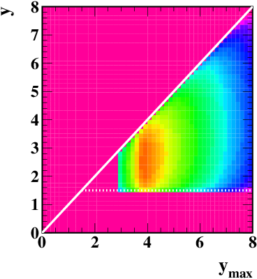
Figure 2 (right) shows the $e^{+}$-$e^{-}$ FF ensemble in the left panel multiplied by a pQCD parton (power-law) spectrum on $y_{max}$ [2]. The most-probable jet (minijet) energy is $E_{jet}\approx 3$ GeV ($y_{max}\approx$ 3.75) consistent with measured jet systematics [9, 3, 2]. That distribution is the argument of a pQCD folding integral (factorization, Bayes’ theorem). Projection onto the vertical axis (integration over the parton spectrum on $y_{max}$) produces a fragment distribution—a pQCD prediction for the measured TCM spectrum hard component $H(y_{t})$ [2]. The hard components of 2D TA correlations may be compared quantitatively with the FF data in Fig. 2. Such comparisons should establish the kinematic limits for jet manifestations in high-energy nuclear collisions.

Correlation structures on $(\eta_{\Delta},\phi_{\Delta})$ and $y_{t}\times y_{t}$ from 200 GeV NSD $p$-$p$ collisions [13, 14] are consistent with extrapolation of the centrality systematics of angular correlations from Au-Au collisions [3]. Both angular correlations and correlations on transverse rapidity are described accurately by the TCM (aside from small-amplitude structures representing Bose-Einstein correlations and gamma conversion to $e^{+}$-$e^{-}$ pairs).

The soft component of 2D angular correlations is represented by a narrow 1D Gaussian on $\eta_{\Delta}$. Soft-component pairs are exclusively the unlike-sign (US) charge combination consistent with projectile-proton dissociation (mainly to gluons near mid-rapidity), and the r.m.s. peak width on $\eta_{\Delta}$ is $\sigma_{soft}\approx 0.5$ [13]. The hard-component 2D peak on $y_{t}\times y_{t}$ corresponds approximately (when projected onto 1D $y_{t}$) to the 1D SP spectrum hard component $H_{0}(y_{t})$ of Eq. (1). The hard component of 2D angular correlations (two features) is consistent with expectations for intra-jet correlations (SS 2D peak, “jet cone”) and inter-jet correlations (AS 1D peak on azimuth, back-to-back jets). The volume of the SS 2D peak corresponds quantitatively to the hard component of the total hadron yield inferred from $y_{t}$ spectrum data and to pQCD calculations [21]. Measured $p$-$p$ angular correlations [13] show only semiquantitative agreement with the pythia Monte Carlo [29].

Single-particle spectrum hard components (jet fragment distributions) are 1D projections of more-complex extended objects (dijets). We seek to isolate 2D trigger-associated hard components that reveal further details of jet structure, especially the analog between TA conditional distributions on space $(y_{ta},y_{tt})$ inferred from $p$-$p$ collisions and parton-fragment conditional distributions on space $(y,y_{max})$ inferred from $e^{+}$-$e^{-}$ collisions [6, 2].

The TA pair distribution for given $n_{ch}$ class is denoted by $F(y_{ta},y_{tt},n_{ch})$. To extract a 2D hard component from TA data we require a 2D soft-component model. Equation (1) is a TCM for SP $y_{t}$ spectra from which the 1D hard component $H(y_{t})$ was isolated. Deriving a TCM for the 2D TA distribution is an exercise in compound probabilities and random sampling from multiple parent distributions. Trigger and associated particles are approximately random samples from fixed spectrum components $S_{0}(y_{t})$ and $H_{0}(y_{t})$ in Eq. (1).

We assume that the soft component of the TA TCM is factorizable (uncorrelated samples). We further assume, only for purposes of illustration in this study, that the 2D hard-component model is also factorizable. We expect that the TA data hard component derived by subtracting the soft-component model is not factorizable in general.

We factorize the 2D TA distribution for given $n_{ch}$ class according to Bayes’ theorem as

where $T(y_{tt})$ is a trigger spectrum and $A(y_{ta}:y_{tt})$ is an ensemble of conditional associated-particle spectra given a trigger at $y_{tt}$. We first obtain a TCM for the 1D trigger spectrum and then develop the 2D TA TCM as a Cartesian product.

We assume that for a given trigger the associated particles are sampled from parent distributions similar to those for the 1D SP spectrum TCM subject to additional marginal constraints described below. For multiplicity class $n_{ch}$ the total number of triggers is $N_{evt}(n_{ch})$, the associated-particle number per event is $n_{ch}-1$, and the total trigger-associated pair number for the given $n_{ch}$ class (excluding self pairs) is $N_{evt}(n_{ch})(n_{ch}-1)$.

We assume that the expressions for soft and hard event types are linearly independent, and event types occur with probabilities $P_{x}(n_{ch})$ as defined previously. We then have $F(y_{ta},y_{tt})=P_{s}F_{s}(y_{ta},y_{tt})+P_{h}F_{h}(y_{ta},y_{tt})$. According to Bayes’ theorem the probability of a TA pair $F_{x}(y_{ta},y_{tt})$ can be written as the product of trigger probability $T_{x}(y_{tt},n_{ch})$ and $A_{x}(y_{ta}:y_{tt},n_{ch})$, the conditional probability of an associated particle at $y_{ta}$ given a trigger at $y_{tt}$. $A_{x}(y_{ta}:y_{tt})$ is based on the $F_{x}(y_{t})$ from the 1D SP TCM but is set to zero above $y_{tt}$ (void). Combining the conditional probabilities with the corresponding trigger-spectrum components we obtain a 2D TCM for unit-normal $F(y_{ta},y_{tt},n_{ch})$

where $A_{s}(y_{ta}:y_{tt},n_{ch})=S_{0}^{\prime\prime}(y_{ta}:y_{tt},n_{ch})$ for soft and $A_{h}(y_{ta}:y_{tt},n_{ch})=p_{s}^{\prime}(n_{ch})S_{0}^{\prime}(y_{ta}:y_{tt},n_{ch})+p_{h}^{\prime}(n_{ch})H_{0}^{\prime}(y_{ta}:y_{tt},n_{ch})$ for hard event types. Primes indicate that the conditional probabilities may deviate from the corresponding 1D SP spectrum models because of imposed marginal constraints. Modifications to the SP spectrum components are represented by $O(1)$ weight functions $D_{x}(y_{tt})$ and $E_{x}(y_{ta})$ as described in App. A. Note that for associated samples $p_{x}^{\prime}=n_{x}^{\prime}/(n_{ch}-1)$.

Figure 5 shows the predicted TCM $F(y_{ta},y_{tt},n_{ch})$ simulating measured 2D TA correlations for four $p$-$p$ multiplicity classes. The rapidity interval $y_{t}\in[1,4.5]$ is divided into 25 histogram bins consistent with previous $y_{t}\times y_{t}$ data analysis [13, 14]. The hard components of measured 2D TA distributions should relate to the jet systematics of Fig. 2. The soft components of the TCM defined by Eq. (10) may be used to isolate TA data hard components for such comparisons. We now consider details of the conditional distributions $A_{x}(y_{ta}:y_{tt},n_{ch})$.

The 2D TA distribution $F(y_{ta},y_{tt},n_{ch})$ must integrate over $y_{ta}$ to the unit-normal trigger spectrum $T(y_{tt},n_{ch})$ and over $y_{tt}$ to the unit-normal SP spectrum $F(y_{ta},n_{ch})$ (minus the trigger spectrum if self pairs are excluded). Those marginal constraints modulate the conditional distributions $A_{x}(y_{ta}:y_{tt})$ in the 2D TA TCM and must be met separately for soft and hard events. We seek the most general 2D model functions that satisfy the constraints.

For event-type $x$ a sum over all events (triggers) should return the 1D parent spectrum $F_{x}(y_{t})$, but we exclude self pairs (triggers) from the 2D TA distribution. Since the trigger self pairs appear along the main diagonal they are described on $y_{ta}$ by the same function $T_{x}(y_{ta},n_{ch})$. The complement is the unit-normal marginal spectrum of associated particles $A_{x}(y_{ta})$ defined for given $n_{ch}$ by

The following must be true for independent sampling from SP parent distribution $F_{x}(y_{t})$ for given $n_{ch}$

Each associated-particle conditional probability should be unit normal on $y_{ta}$ for any $y_{tt}$

so that integration of Eq. (12) over $y_{ta}$ returns Eq. (9). Equations (12) and (13) define the required marginal constraints on the 2D conditional probability distributions.

Conditional distributions $A_{x}(y_{ta}:y_{tt})$ can be obtained by an iterative process. We refer to histogram $A_{x}(y_{ta}:y_{tt})$ as having rows indexed by $y_{ta}$ and columns indexed by $y_{tt}$. To form the initial approximation to $A_{x}(y_{ta}:y_{tt})$ 1D distribution $F_{x}(y_{ta})$ from the SP TCM is set to zero above $y_{tt}$ for each $y_{tt}$. Equation (13) is imposed for each $y_{tt}$ to renormalize the corresponding column. Equation (12) is then imposed for each $y_{ta}$ to renormalize the corresponding row, which may change the column normalizations. The resulting alteration of SP model functions $F_{x}$ is represented by weight functions $D_{x}$ and $E_{x}$. Iteration converges rapidly and a single pass provides sufficient accuracy within the kinematic region on $(y_{ta},y_{tt})$ relevant to the TA hard component. Further details are presented in App. A.

Figure 6 illustrates the effects of marginal constraints on $S_{0}^{\prime\prime}(y_{ta}:y_{tt})$ (left) and $H_{0}^{\prime}(y_{ta}:y_{tt})$ (right). The initial $A_{x}(y_{ta}:y_{tt})$ forms follow the SP parent spectra $F_{x}(y_{t})$ on $y_{ta}$ and are uniform on $y_{tt}$ subject to the condition $y_{ta}<y_{tt}$. The constraint of Eq. (13) represented by $D_{x}(y_{tt})$ causes elevated amplitudes at smaller $y_{tt}$ due to the reduced acceptance on $y_{ta}$. The constraint of Eq. (12) represented by $E_{x}(y_{ta})$ might alter amplitudes at larger $y_{ta}$ relative to the SP parents. Any renormalization on $y_{ta}$ could then disturb the normalization on $y_{tt}$ requiring multiple iterations for convergence, but we observe that such effects are negligible. Systematic uncertainties for the renormalizations are discussed in Sec. VII.

References

- [1] T. A. Trainor, Phys. Rev. D 87, 054005 (2013).
- [2] T. A. Trainor, Phys. Rev. C 80, 044901 (2009).
- [3] G. Agakishiev, et al. (STAR Collaboration), Phys. Rev. C 86, 064902 (2012).
- [4] M. Z. Akrawy et al. (OPAL Collaboration) Phys. Lett. B, 247, 617 (1990).
- [5] W. Braunschweig et al. (TASSO Collaboration), Z. Phys. C 47, 187 (1990).
- [6] T. A. Trainor and D. T. Kettler, Phys. Rev. D 74, 034012 (2006).
- [7] J. Adams et al. (STAR Collaboration), Phys. Rev. D 74, 032006 (2006).
- [8] T. Affolder et al. (CDF Collaboration), Phys. Rev. D 65, 092002 (2002).
- [9] C. Albajar et al. (UA1 Collaboration), Nucl. Phys. B 309, 405 (1988).
- [10] M. M. Aggarwal et al. (STAR Collaboration), Phys. Rev. C 82, 024912 (2010).
- [11] T. A. Trainor, Phys. Rev. C 81, 014905 (2010).
- [12] J. Adams et al. (STAR Collaboration), Phys. Rev. C 73, 064907 (2006).
- [13] R. J. Porter and T. A. Trainor (STAR Collaboration), J. Phys. Conf. Ser. 27, 98 (2005).
- [14] R. J. Porter and T. A. Trainor (STAR Collaboration), PoS C FRNC2006, 004 (2006).
- [15] T. A. Trainor, Int. J. Mod. Phys. E 17, 1499 (2008).
- [16] R. Field, Acta Phys. Polon. B 42, 2631 (2011).
- [17] J. Adams et al. (STAR Collaboration), Phys. Rev. C 72, 014904 (2005).
- [18] T. A. Trainor, J. Phys. G 40, 055104 (2013).
- [19] T. A. Trainor, Mod. Phys. Lett. A 23, 569 (2008).
- [20] M. M. Aggarwal et al. (STAR Collaboration), Phys. Rev. C 83, 034910 (2011).
- [21] T. A. Trainor and D. T. Kettler, Phys. Rev. C 83, 034903 (2011).
- [22] J. Adams et al. (STAR Collaboration), Phys. Lett. B 634, 347 (2006).
- [23] T. A. Trainor, R. J. Porter and D. J. Prindle, J. Phys. G 31, 809 (2005).
- [24] D. Kharzeev and M. Nardi, Phys. Lett. B 507, 121 (2001).
- [25] T. A. Trainor, D. T. Kettler, D. J. Prindle and R. L. Ray, arXiv:1302.0300.
- [26] M. Bahr, S. Gieseke, M. A. Gigg, D. Grellscheid, K. Hamilton, O. Latunde-Dada, S. Platzer and P. Richardson et al., Eur. Phys. J. C 58, 639 (2008).
- [27] M. Bahr, J. M. Butterworth and M. H. Seymour, JHEP 0901, 065 (2009).
- [28] X.-N. Wang, Phys. Rev. D 46, R1900 (1992); X.-N. Wang and M. Gyulassy, Phys. Rev. D 44, 3501 (1991).
- [29] T. Sjöstrand and M. van Zijl, Phys. Rev. D 36, 2019 (1987); T. Sjöstrand, Comput. Phys. Commun. 82, 74 (1994); T. Sjöstrand, L. Lönnblad, S. Mrenna and P. Skands, hep-ph/0308153.
- [30] S.-y. Li and X.-N. Wang, Phys. Lett. B 527, 85 (2002).
- [31] T. A. Trainor, arXiv:1303.4774.
- [32] I. M. Dremin and J. W. Gary, Phys. Rept. 349, 301 (2001).
- [33] M. S. Alam et al. (CLEO Collaboration), Phys. Rev. D 56, 17 (1997).
- [34] B. I. Abelev et al. (STAR Collaboration), Phys. Rev. C 81, 054907 (2010).
- [35] M. M. Aggarwal et al. (STAR Collaboration), Phys. Rev. C 82, 024912 (2010).
- [36] T. Affolder et al. (CDF Collaboration), Phys. Rev. D 65, 092002 (2002).
- [37] V. Khachatryan et al. (CMS Collaboration), Eur. Phys. J. C 70, 555 (2010).