Improving A^⋆OMP: Theoretical and Empirical Analyses
With a Novel Dynamic Cost Model

The fundamental goal of compressed sensing (CS) is to unify data acquisition and compression by observing a lower dimensional vector $\mathbf{y}=\mathbf{\Phi}\mathbf{x}$ instead of the signal $\mathbf{x}$, where $\mathbf{\Phi}\in{\mathbb{R}}^{M\times{N}}$ is the (generally random) measurement matrix¹¹ 1 A more general model involves a structured dictionary $\mathbf{\Psi}$ for sparse representation of $\mathbf{x}$, i.e., $\mathbf{x}=\mathbf{\Psi}\mathbf{z}$ where $\mathbf{z}$ is sparse and $\mathbf{x}$ is not. In this more general case, observation model can be written as $\mathbf{y}=\mathbf{\Phi}\mathbf{\Psi}\mathbf{z}$. For simplicity, we omit $\mathbf{\Psi}$ and treat $\mathbf{x}$ as sparse., $\mathbf{y}\in{\mathbb{R}}^{M}$, and $\mathbf{x}\in{\mathbb{R}}^{N}$. The dimensionality reduction follows $M<N$, as a result of which $\mathbf{x}$ cannot be directly solved back from $\mathbf{y}$. Alternatively, assuming $\mathbf{x}$ is $K$-sparse (i.e., it has at most $K$ nonzero components), or compressible, $\mathbf{x}$ can be recovered under certain conditions by solving

where $\|\mathbf{x}\|_{0}$ denotes the number of nonzero elements in $\mathbf{x}$.

As the direct solution of (1) is intractable, approximate solutions have emerged in the CS literature. Convex optimization algorithms [6, 7, 8, 9] relax (1) by replacing $\|\mathbf{x}\|_{0}$ with its closest convex approximation $\|\mathbf{x}\|_{1}$. Greedy algorithms [2, 10, 11, 12, 13, 14] provide simple and approximate solutions via iterative residue minimization. Other recovery schemes include Bayesian methods [15, 16], nonconvex approaches [17, 18, 19, 20], iterative reweighted methods [21, 22, 23], etc.

OMP is among the most acknowledged greedy algorithms for sparse recovery [24, 25, 26]. It aims at iterative detection of the support, i.e., the set of indices corresponding to nonzero coefficients, of $\mathbf{x}$. At each iteration, OMP identifies the best match to the residue of $\mathbf{y}$ among the atoms, i.e., columns of $\mathbf{\Phi}$, by choosing the index of the atom with maximum correlation. That is, OMP is structurally based on continuous expansion of a single hypothesis, represented by a single iteratively-expanded support estimate, or path.

On the other hand, simultaneous evaluation of multiple hypotheses for the sparse support may improve recovery over the single-path algorithms like OMP. Multiple hypotheses may be represented by a search tree, and the recovery problem can be efficiently solved by sophisticated best-first search techniques. To promote this idea, the authors have introduced the A^⋆OMP algorithm [1, 5] which is an iterative semi-greedy approach that utilizes A^⋆ search on a multiple hypotheses search tree in order to find an approximation of (1). The nodes of the tree contain indices of the selected atoms, and the paths represent the candidate support sets for $\mathbf{x}$. Figure 1 illustrates the evaluation of such a tree in comparison to OMP. At each iteration, A^⋆OMP first selects the best path with the minimum cost criterion which depends on the $\ell_{2}$ norm of the path residue. Then, the best path is expanded by exploring $B$ of its child nodes with maximum correlation to the path residue. That is, $B$ new candidate support sets are appended to the tree. The filled nodes in Figure 1 indicate the child nodes explored per step, which are referred to as $\Delta\mathcal{T}$ in the rest.

In Figure 1, although the OMP solution is among the hypotheses in the tree, A^⋆OMP returns a different support set. In fact, if OMP were successful, A^⋆OMP would also return the same solution. This typical example of OMP failure, where the best-first search identifies the true solution by simultaneous evaluation of multiple hypotheses, illustrates how the multiple path strategy improves the recovery.

Despite this simple illustration, combining the A^⋆ search with OMP is not straightforward. It necessitates properly defined cost models which enable the A^⋆ search to perform the stage-wise residue minimization in an intelligent manner, and effective pruning techniques which make the algorithm tractable. Various structures are introduced in [1] and [5] for the cost model, which is vital for the comparison of paths with different lengths. Pruning strategies, which enable a complexity-accuracy trade-off together with the cost model, are detailed in [1]. Below, we provide a summary of A^⋆OMP, and refer the interested reader to [1] and [5] for the details.

The manuscript at hand concentrates on detailed analyses of the sparse signal recovery performance of A^⋆OMP. Particularly, we concentrate on the variant AMul-A^⋆OMP_e which extends the general form in [1] by the novel AMul cost model from [5] and residue-based termination. We present new theoretical and empirical results to demonstrate the superiority of this variant not only over the A^⋆OMP variants in [1], but also over some conventional sparse recovery methods. Note that AMul-A^⋆OMP_e has only been preliminarily tested in [5] by a set of limited simulations, which are far away from providing enough evidence to generalize its performance. This manuscript presents a detailed empirical investigation of AMul-A^⋆OMP_e, without which the performance analyses would not be complete. These simulations significantly enrich the findings of [5] by previously unpublished results which include phase transition comparisons for different signal statistics, demonstration on an image, a faster hybrid approach and optimality analyses. The results reveal not only the superior recovery accuracy of AMul-A^⋆OMP_e, but also the improvements in the speed of the algorithm due to the residue-based termination and the AMul cost model.

On the other hand, our theoretical findings not only include RIP-based exact recovery guarantees for exact recovery of sparse signals via A^⋆OMP_K and A^⋆OMP_e, but also provide means for comparison of different termination criteria. The former states RIP conditions for the exact recovery of sparse signals from noise-free measurements, while the latter addresses the recovery improvements when the residue-based termination is employed instead of the sparsity-based one. For the analyses, we employ a method similar to the analyses of the OMP algorithm in [26] and [29]. In Section 2.3, we develop a RIP condition for the success of a single A^⋆OMP iteration, which forms a basis for the following theoretical analyses. In Section 2.4, we derive a general recovery condition for exact recovery via A^⋆OMP_K. As intuitively expected, this condition is less restrictive than the $K$-step OMP recovery condition [26]. Section 2.5 presents a very similar general condition for exact recovery via A^⋆OMP_e. In addition, we establish an online recovery condition for exact recovery of a signal with A^⋆OMP_e. Section 2.7 compares the general and online recovery conditions, clarifying that the latter is less restrictive. This suggests that A^⋆OMP_e possesses stronger recovery capabilities than A^⋆OMP_K.

Section 3 compares the recovery accuracy of AMul-A^⋆OMP_e to other A^⋆OMP variants, basis pursuit (BP) [6], subspace pursuit (SP) [10], OMP [2], iterative hard thresholding (IHT) [11], iterative support detection (ISD) [21], smoothed $\ell_{0}$ (SL0) [17], MMP [28], and forward-backward pursuit (FBP) [12]. The main contribution is the phase transitions which are obtained by computationally expensive experiments for different signal types. These generalize the strong recovery capability of AMul-A^⋆OMP_e over a wide range of $N$, $M$ and $K$. We investigate the recovery rates and average recovery error as well. Run times illustrate the acceleration with the AMul cost model and the residue-based termination. An hybrid of A^⋆OMP_e and OMP demonstrates how the recovery speed can be improved without losing the accuracy. The sparse image recovery problem represents a more realistic coefficient distribution than the other artificial examples.

Restricted isometry property (RIP) [7] provides an important means for theoretical guarantees in sparse recovery problems. A matrix $\mathbf{\Phi}$ is said to satisfy the $L$-RIP if there exists a restricted isometry constant (RIC) $\delta_{L}\in(0,1)$ satisfying

Some random matrices, such as Gaussian or Bernoulli matrices, satisfy the $L$-RIP with high probabilities if $L$, $M$ and $N$ satisfy some specific conditions [30, 31]. Exploiting this property, RIP has been utilized to obtain recovery guarantees for sparse recovery algorithms [7, 31, 29, 32, 33].

We now present some preliminary lemmas based on RIP:

We define the success of an A^⋆OMP iteration as $\Delta\mathcal{T}$ containing at least one correct index, i.e., $\Delta\mathcal{T}\cap\{\mathcal{T}-\mathcal{T}^{b}\}\neq\emptyset$. The following theorem guarantees the success of an iteration:

Below, Theorem 1 is used as a basis for exact recovery. Note that we assume $\sqrt{B}\leq\sqrt{K-n_{c}}$ in the rest and skip the term $\frac{1}{2}$ in Theorem 1 for simplicity. This can be justified by the fact that $B$ is chosen small (such as 2 or 3) in practice.

First, let us introduce some definitions:

Optimal path: Path $i$ is said to be optimal if $\mathcal{T}^{i}\subset\mathcal{T}$.

Optimal pruning: Pruning is defined as optimal if it does not remove all optimal paths from the tree.

Figure 2 illustrates the optimality notion with a typical example. Indices from the true support are shown by the filled nodes. The optimal paths, which contain filled nodes only, are designated with ‘+’. Since $K_{\text{max}}=K=4$, the paths become complete with four nodes. The nodes which are pruned due to $P=3$ are crossed. Step 3 exemplifies the optimal pruning. Though an optimal path is pruned, there still remains another optimal one. Expanding this optimal path in Step 5, the search obtains the true solution represented by the complete and optimal path $\{3,4,6,2\}$.

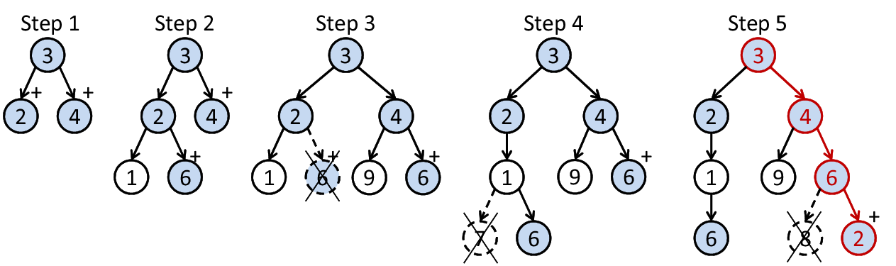
Now, we present the exact recovery condition for A^⋆OMP_K:

Note that the condition $\varepsilon=0$, stated in Theorem 2 for the sake of theoretical correctness, translates into a very small $\varepsilon$ in practice to account for the numerical computation errors.

We observe that the $K$-step exact recovery condition of OMP, $\delta_{K+1}<1{\big/}\big(\sqrt{K}+1\big)$, is a special case of Theorem 2 when $B=I=1$. Moreover, when the bounds for OMP and A^⋆OMP_K are compared, (12) is clearly less restrictive, which explains the improved recovery accuracy of A^⋆OMP_K.

Theorem 2 is closely related to the theoretical analysis of MMP in [28]. It can be trivially shown that Theorem 2 is also applicable to MMP. Moreover, it implies a better, i.e., less restricted, recovery condition when compared to [28], where the condition is stated as $\delta_{K+B}<1{\big/}\big(\sqrt{K}+2\sqrt{B}\big)$.

We extend the definitions in the previous section for A^⋆OMP_e where $K_{\text{max}}>K$. First, note that path $i$ is now complete if $l^{i}=K_{\text{max}}>K$. Next, we introduce the following definitions:

Potentially-optimal path: A path is said to be potentially-optimal (p-optimal) if $n_{f}\leq K_{\text{max}}-K$. A p-optimal path can be expanded into a superset of $\mathcal{T}$ with at most $K_{\text{max}}$ nodes. Note that an optimal path is a special case where $K_{\text{max}}=K$.

Potentially-optimal pruning: Pruning is defined as p-optimal if it does not remove all p-optimal paths from the search tree.

Figure 3 depicts some examples of p-optimality and completeness. Clearly, a path is p-optimal only if a superset of $\mathcal{T}$ is among its extensions. Moreover, path 1 reveals that the optimal and p-optimal path notions are equal when $n_{f}=0$.

Next, we state the following lemma:

Now an online recovery condition can be presented for A^⋆OMP_e:

Note that the condition $\varepsilon=0$, stated in Theorem 3 for the sake of theoretical correctness, translates into a very small $\varepsilon$ in practice to account for the numerical computation errors.

Since Theorem 3 depends on the existence of a p-optimal path satisfying (15), it does not provide overall guarantees for all $K$-sparse signals as Theorem 2 does. In contrast, Theorem 3 implies online guarantees depending on the support estimates of the intermediate (i.e., neither complete nor empty) p-optimal paths. In fact, it is hardly possible to provide guarantees for the existence of such paths. Nonetheless, Theorem 3 can be generalized starting with the empty path:

We omit the proof of Theorem 4, since it follows trivially from Theorem 3 by replacing $n_{f}=n_{c}=0$.

Theorem 4 provides overall guarantees for all sparse signals as Theorem 2. We observe that both theorems require the same RIP condition for exact recovery of all sparse signals.

Although Theorem 2 and Theorem 4 provide similar overall guarantees, A^⋆OMP_e also possesses the online guarantees of Theorem 3. Section 2.7 presents an analytical comparison of the conditions in Theorem 3 and Theorem 4. This study states that Theorem 3 may be satisfied even when Theorem 4 fails. This reveals the importance of the online guarantees to comprehend the improved recovery accuracy of A^⋆OMP_e.

Theorem 2 and Theorem 4 both rely on optimal/p-optimal pruning, which is hard to prove analytically. Though this may be seen as a limitation of the theoretical findings, it is obvious that pruning is unavoidable for the tractability of the search. As an empirical justification, it is important to observe that the true solution may be reached along different paths in the tree. This is due to the fact that the ordering of the nodes is not important. Hence, the tree is subject to contain a large number of candidate solutions (optimal/p-optimal paths), while it is enough for exact recovery when only one of these optimal paths is not pruned.

Moreover, the theoretical analysis of MMP in [28] is also subject to an equivalent assumption in practice. Though the authors analyse MMP without any limit on the number of explored paths, they acknowledge that this is impractical. Similar to A^⋆OMP, they limit the number of paths for the empirical evaluation of MMP. It is clear that the theoretical findings of [28], which do not address this pruning strategy, are practically meaningful only with an assumption on pruning.

To address the validity of the online condition in Theorem 3, we show that it can be satisfied when the overall guarantees in Theorem 4 fail. The next theorem reveals that a p-optimal path satisfying (15) may be found even when (16) fails.

Theorem 5 clarifies that Theorem 3 may hold even when Theorem 4 fails. In other words, A^⋆OMP_e possesses online guarantees for some sparse signals for which the overall guarantees fail. This explains why A^⋆OMP_e improves the recovery accuracy over A^⋆OMP_K, and reveals that the residue-based termination is more optimal for noise-free sparse signal recovery than its sparsity-based counterpart.

Note that Theorem 5 is based on some $n_{f}$, $n_{c}$ and $K$ ranges for which it is provable. This is enough, since even a single supporting case already establishes the validity of Theorem 3. On the other hand, we expect it to be valid for a wider range. This intuition is also supported by the following simulations, where A^⋆OMP_e improves recovery in almost all cases.

Unless given explicitly, the setup is as follows: We set $I=3$, $B=2$ and $P=200$. For A^⋆OMP_e, $\varepsilon$ is set to $10^{-6}$. This $\varepsilon$ is shared by OMP, which also runs until $\|\mathbf{r}\|_{2}\leq\varepsilon\|\mathbf{y}\|_{2}$. We select $\alpha_{\text{Mul}}=0.8$ for Mul-A^⋆OMP_K, $\alpha_{\text{Mul}}=0.9$ for Mul-A^⋆OMP_e and $\alpha_{\text{AMul}}=0.97$ for AMul-A^⋆OMP_e. We employ FBP with $\alpha=0.2M$ and $\beta=\alpha-1$ as suggested in [12]. For MMP-DF, we set the branching factor $L=6$ following [28], and allow a maximum of 200 paths for a fair comparison with the A^⋆OMP variants where $P=200$. Each test is repeated over a randomly generated set of $S$ sparse samples. For each sample, $\mathbf{\Phi}$ is drawn from the Gaussian distribution with mean zero and standard deviation $1/N$. The nonzero entries of the test samples are selected from three random ensembles. The nonzero entries of the Gaussian sparse signals follow standard Gaussian distribution while those of the uniform sparse signals are distributed uniformly in $[-1,1]$. The constant amplitude random sign (CARS) sparse signals have unit magnitude nonzero elements with random sign. The average normalized mean-squared-error (ANMSE) is defined as

where $\hat{\mathbf{x}}_{i}$ is the recovery of the $i$th test vector $\mathbf{x}_{i}$.

We perform the A^⋆OMP recovery using the AStarOMP software⁶⁶ 6 Available at http://myweb.sabanciuniv.edu/karahanoglu/research/.. AStarOMP implements the A^⋆ search by an efficient trie⁷⁷ 7 Trie is an ordered tree data structure in computer science. The ordering provides important advantages for the implementation of A^⋆OMP, such as reducing the cost of addition/deletion of paths and finding equivalent paths. structure [34], where the nodes are ordered with priorities proportional to their inner products with $\mathbf{y}$. This maximizes the number of shared nodes between paths, allowing a more compact tree representation and faster tree modifications. The orthogonal projection is performed via the QR factorization.

The first simulation deals with the recovery of Gaussian sparse signals, where $N=256$, $M=100$, $K\in[10,50]$, $K_{\text{max}}=55$ and $S=500$. The results are depicted in Figure 4, which reveals that A^⋆OMP performs significantly better than the other algorithms. A^⋆OMP_e provides exact recovery until $K=40$, which is clearly the best. We observe similar ANMSE among A^⋆OMP variants, while the residue-based termination improves the exact recovery rates significantly. Evidently, A^⋆OMP_e is better than A^⋆OMP_K at identifying smaller magnitude entries, which hardly change the ANMSE, however increase the exact recovery rates. It is also important that all A^⋆OMP variants yield higher recovery rates than MMP-DF. Especially, Mul-A^⋆OMP_K and MMP-DF are interesting to compare since both return solutions with $K$ indices. We observe that Mul-A^⋆OMP_K yields significantly higher recovery rates than MMP-DF, which implies the effectiveness of the sophisticated search techniques employed in A^⋆OMP.

As for the average run times⁸⁸ 8 OMP and A^⋆OMP are tested using the AStarOMP software. The other algorithms are ignored as they run in MATLAB, which is slower., both the residue-based termination and the AMul cost model significantly accelerate A^⋆OMP due to the relaxation of $\alpha$ to larger values. Since AMul-A^⋆OMP_e can afford the largest $\alpha$, it is the fastest A^⋆OMP variant. This confirms the claim in Section 1.2 that increasing $\alpha$ reduces the number of explored nodes and accelerates A^⋆OMP.

In addition to this example, [5] contains simulations for uniform and binary sparse signals and noisy measurements. These simulations indicate that AMul-A^⋆OMP_e improves the recovery for uniform sparse signals and noisy cases as well.

Empirical phase transitions provide important means for recovery analysis, since they reveal the recovery performance over the feasible range of $M$ and $K$. Consider the normalized measures $\lambda=M/N$ and $\rho=K/M$. The phase transition curve is mostly a function of $\lambda$ [35], hence it allows for a general characterization of the recovery performance.

To obtain the phase transitions, we fix $N=250$, and alter $M$ and $K$ to sample the $\{\lambda,\rho\}$ space for $\lambda\in[0.1,0.9]$ and $\rho\in[0,1]$. For each $\{\lambda,\rho\}$ tuple, we randomly generate 200 sparse instances and perform the recovery. Setting the exact recovery criterion as $\frac{\|\mathbf{x}_{i}-\hat{\mathbf{x}}_{i}\|_{2}}{\|\mathbf{x}_{i}\|_{2}}\leq 10^{-2}$, we count the exactly recovered samples. The phase transitions are then obtained as in [35]. For each $\lambda$, we employ a generalized linear model with logistic link to describe the exact recovery curve over $\rho$, and then find $\rho$ which yields $50\%$ exact recovery probability. Combination of these $\rho$ values gives the phase transition curve.

Let us first concentrate on $K_{\text{max}}$ and define the normalized measure $\rho_{\text{max}}=K_{\text{max}}{\big/}M$. Once we identify the optimal $\rho_{\text{max}}$ over $\lambda$, we can set $K_{\text{max}}$ for particular $\lambda$ and $M$. To find the optimal $\rho_{\text{max}}$, we have run a number of simulations and observed that the recovery performance of AMul-A^⋆OMP_e is quite robust to $\rho_{\text{max}}$, with a perturbation up to $3\%$. Hence, the recovery accuracy is mostly independent of $\rho_{\text{max}}$. Yet, based on our experience, we set $\rho_{\text{max}}=0.5+0.5\lambda$ taking into account both the accuracy and complexity of the search.

Figure 5 depicts the phase transition curves. Clearly, AMul-A^⋆OMP_e yields better phase transitions than the other algorithms for the Gaussian and uniform sparse signals. We also observe that FBP provides fast approximations with better accuracy than BP and the two other greedy competitors, SP and OMP for these two cases. This reveals that FBP is actually suitable to applications where speed is crucial. On the other hand, BP and ISD are the best performers for the CARS case, while AMul-A^⋆OMP_e is the third best. We observe that BP is robust to the coefficient distribution, while the phase transitions for AMul-A^⋆OMP_e and OMP exhibit the highest variation among distributions. This indicates that OMP-type algorithms are more effective when the nonzero elements span a wide magnitude range such as the Gaussian distribution. Moreover, if this range gets wide enough, even OMP can outperform BP. In parallel, the CARS ensemble is referred to as the most challenging case for the greedy algorithms in the literature [10, 35]. This can be understood analytically by considering the span of the correlation between $\mathbf{\Phi}_{\mathcal{T}}$ and $\mathbf{y}$. The detailed analytical analysis in [36] state that this span gets smaller when the magnitudes of the nonzero elements get closer, and vice versa. When this span gets smaller (for the CARS ensemble in the limit), wrong indices are more likely to be selected by OMP, increasing the failure rate.

We have observed that OMP provides exact recovery up to some mid-sparsity range. Moreover, there are regions where AMul-A^⋆OMP_e provides exact recovery while OMP recovery rates are also quite high. In these regions, we can accelerate the recovery without sacrificing the accuracy by a two-stage hybrid scheme. We first run OMP, and then AMul-A^⋆OMP_e only if OMP fails. Assuming that ${K{+}K_{\text{max}}}$-RIP holds, a non-vanishing residue indicates OMP failure, and then AMul-A^⋆OMP_e is run. This reduces the number of AMul-A^⋆OMP_e runs and accelerates the recovery. Moreover, we use the order by which OMP chooses the vectors for setting the priorities of trie nodes. A vector OMP chooses first gets higher priority, and is placed at lower levels of the trie. This reduces not only the trie size but also trie modification costs.

According to the recovery results in Figure 6, AMul-A^⋆OMP_e and the hybrid approach yield identical exact recovery rates, while the latter is significantly faster. This acceleration is proportional to the exact recovery rate of OMP. That is, the hybrid approach is faster where OMP is better. These results show that this approach is indeed able to detect the OMP failures, and run AMul-A^⋆OMP_e only for those instances.

To illustrate AMul-A^⋆OMP_e on a more realistic coefficient distribution, we demonstrate recovery of some commonly used $512\times 512$ images including ‘Lena’, ‘Tracy’, ‘Cameraman’, etc. The recovery is performed in $8\times 8$ blocks in order to break the problem into smaller and simpler subproblems. Each image is first preprocessed to obtain $K$-sparse blocks in the 2D Haar Wavelet basis $\mathbf{\Psi}$ by keeping the $K$ largest magnitude wavelet coefficients for each block⁹⁹ 9 This formulation involves the structured dictionary $\mathbf{\Psi}$ for sparse representation of the images. The observation model becomes $\mathbf{y}=\mathbf{\Phi}\mathbf{\Psi}\mathbf{x}$, where the reconstruction basis is not $\mathbf{\Phi}$ alone, but $\mathbf{\Phi}\mathbf{\Psi}$.. We select $K=12$ for the image ’Bridge’, and $K=14$ for the rest. $M=32$ observations are taken from each block. The entries of $\mathbf{\Phi}$ are randomly drawn from the Gaussian distribution with mean 0 and standard deviation $1/N$. We set $I=3$, $P=200$ and $K_{\text{max}}=20.$ $\alpha_{\text{AMul}}$ is reduced to 0.85 in order to compensate the decrement in the auxiliary term of (2) due to smaller $K_{\text{max}}$. Peak Signal-to-Noise Ratio (PSNR) values obtained by employing different recovery algorithms are given in Table 2. For each image, maximum and minimum PSNR values obtained are shown in bold and in italics, respectively. Mean PSNR for each algorithm is also given on the last row. AMul-A^⋆OMP_e exhibits significant improvements over the competitors and yields the maximum PSNR for all images tested. Increasing $B$ from 2 to 3 further improves PSNR, yielding improvements of 15.7 dB over BP, 15.3 dB over ISD, 17.7 dB over SL0, and 11.7 dB over MMP-DF on the average. As a visual example, we depict the reconstruction of the test image “Bridge” using BP and AMul-A^⋆OMP_e with $B=3$ in Figure 7. In this case, BP yields 29.9 dB PSNR, while AMul-A^⋆OMP_e improves the PSNR to 51.4 dB. Though not depicted in Figure 7, AMul-A^⋆OMP_e outperforms BP with 46.8 dB when $B=2$ as well. A detailed investigation of the recovered images reveals that AMul-A^⋆OMP_e improves the recovery especially at detailed regions and boundaries.

References

- [1] N.B. Karahanoglu and H. Erdogan, “A* orthogonal matching pursuit: Best-first search for compressed sensing signal recovery,” Digital Signal Processing, vol. 22, no. 4, pp. 555–568, July 2012.
- [2] Y.C. Pati, R. Rezaiifar, and P.S. Krishnaprasad, “Orthogonal matching pursuit: Recursive function approximation with applications to wavelet decomposition,” in Proc. 27th Asilomar Conference on Signals, Systems and Computers, Los Alamitos, CA, 1993, vol. 1, pp. 40–44.
- [3] P.E. Hart, N.J. Nilsson, and B. Raphael, “A formal basis for the heuristic determination of minimum cost paths,” IEEE Trans. Syst. Sci. Cybern., vol. 4, no. 12, pp. 100–107, July 1968.
- [4] F. Jelinek, Statistical Methods For Speech Recognition, chapter 6, MIT Press, Cambridge, MA, USA, 1997.
- [5] N.B. .Karahanoglu and H. Erdogan, “A comparison of termination criteria for A*OMP,” in European Signal Processing Conference, Bucharest, Romania, Aug. 2012.
- [6] S. Chen, D. Donoho, and M. Saunders, “Atomic decomposition by basis pursuit,” SIAM J. on Sci. Comp., vol. 20, no. 1, pp. 33–61, 1998.
- [7] E. Candès and T. Tao, “Decoding by linear programming,” IEEE Trans. Inf. Theory, vol. 51, no. 12, pp. 4203–4215, Dec. 2005.
- [8] D. Donoho, “Compressed sensing,” IEEE Trans. Inf. Theory, vol. 52, no. 4, pp. 1289–1306, Apr. 2006.
- [9] J.A. Tropp, “Algorithms for simultaneous sparse approximation. part ii: Convex relaxation,” Signal Processing, vol. 86, no. 3, pp. 589 – 602, 2006, Sparse Approximations in Signal and Image Processing.
- [10] W. Dai and O. Milenkovic, “Subspace pursuit for compressive sensing signal reconstruction,” IEEE Trans. Inf. Theory, vol. 55, no. 5, pp. 2230–2249, May 2009.
- [11] T. Blumensath and M.E. Davies, “Iterative hard thresholding for compressed sensing,” Appl. Comp. Harmonic Anal., vol. 27, no. 3, pp. 265–274, 2009.
- [12] N.B. Karahanoglu and H. Erdogan, “Compressed sensing signal recovery via forward-backward pursuit,” Digital Signal Processing, vol. 23, no. 5, pp. 1539 – 1548, 2013.
- [13] D. Sundman, S. Chatterjee, and M. Skoglund, “Distributed greedy pursuit algorithms,” Signal Processing, vol. 105, no. 0, pp. 298 – 315, 2014.
- [14] J.A. Tropp, A.C. Gilbert, and M.J. Strauss, “Algorithms for simultaneous sparse approximation. part i: Greedy pursuits,” Signal Processing, vol. 86, no. 3, pp. 572–588, Mar. 2006.
- [15] Sç Ji, Y. Xue, and L. Carin, “Bayesian compressive sensing,” IEEE Trans. Signal Process., vol. 56, no. 6, pp. 2346–2356, 2008.
- [16] S.D. Babacan, R. Molina, and A.K. Katsaggelos, “Bayesian compressive sensing using laplace priors,” IEEE Trans. Image Process., vol. 19, no. 1, pp. 53–63, 2010.
- [17] H. Mohimani, M. Babaie-Zadeh, and C. Jutten, “A fast approach for overcomplete sparse decomposition based on smoothed l0 norm,” IEEE Trans. Signal Process., vol. 57, no. 1, pp. 289–301, Jan. 2009.
- [18] M.R. Mohammadi, E. Fatemizadeh, and M.H. Mahoor, “Non-negative sparse decomposition based on constrained smoothed norm,” Signal Processing, vol. 100, no. 0, pp. 42 – 50, 2014.
- [19] L.B. Montefusco, D. Lazzaro, and S. Papi, “A fast algorithm for nonconvex approaches to sparse recovery problems,” Signal Processing, vol. 93, no. 9, pp. 2636 – 2647, 2013.
- [20] T. Ince, A. Nacaroglu, and N.l. Watsuji, “Nonconvex compressed sensing with partially known signal support,” Signal Processing, vol. 93, no. 1, pp. 338 – 344, 2013.
- [21] Y. Wang and W. Yin, “Sparse signal reconstruction via iterative support detection,” SIAM Journal on Imaging Sciences, vol. 3, no. 3, pp. 462–491, 2010.
- [22] E. Candés, M. Wakin, and S. Boyd, “Enhancing sparsity by reweighted minimization,” Journal of Fourier Analysis and Applications, vol. 14, pp. 877–905, 2008.
- [23] J. Fang, Y. Shen, H. Li, and Z. Ren, “Sparse signal recovery from one-bit quantized data: An iterative reweighted algorithm,” Signal Processing, vol. 102, no. 0, pp. 201 – 206, 2014.
- [24] J. A. Tropp and A. C. Gilbert, “Signal recovery from random measurements via orthogonal matching pursuit,” IEEE Trans. Inf. Theory, vol. 53, no. 12, pp. 4655–4666, 2007.
- [25] M.A. Davenport and M.B. Wakin, “Analysis of orthogonal matching pursuit using the restricted isometry property,” IEEE Trans. Inf. Theory, vol. 56, no. 9, pp. 4395–4401, sept. 2010.
- [26] J. Wang and B. Shim, “On the recovery limit of sparse signals using orthogonal matching pursuit,” IEEE Trans. Signal Process., vol. 60, no. 9, pp. 4973–4976, Sept. 2012.
- [27] S.F. Cotter and B.D. Rao, “Application of tree-based searches to matching pursuit,” in Acoustics, Speech and Signal Processing (ICASSP), 2001 IEEE International Conference on, 2001, pp. 3933–3936.
- [28] S. Kwon, J. Wang, and B. Shim, “Multipath matching pursuit,” IEEE Trans. Inf. Theory, vol. 60, no. 5, pp. 2986–3001, May 2014.
- [29] N.B. Karahanoglu and H. Erdogan, “Online recovery guarantees for orthogonal matching pursuit,” 2013, preprint, http://arxiv.org/abs/1210.5991.
- [30] M. Rudelson and R. Vershynin, “Sparse reconstruction by convex relaxation: Fourier and gaussian measurements,” in 40th Annual Conference on Information Sciences and Systems, 2006, pp. 207–212.
- [31] E. Candès and T. Tao, “Near-optimal signal recovery from random projections: universal encoding strategies?,” IEEE Trans. Inf. Theory, vol. 52, no. 12, pp. 5406–5425, 2006.
- [32] W. Xu, Y. Tian, and J. Lin, “Performance analysis of partial segmented compressed sampling,” Signal Processing, vol. 93, no. 9, pp. 2653 – 2663, 2013.
- [33] Y. Wang, J. Wang, and Z. Xu, “Restricted p-isometry properties of nonconvex block-sparse compressed sensing,” Signal Processing, vol. 104, no. 0, pp. 188 – 196, 2014.
- [34] R. Sedgewick and K. Wayne, Algorithms, Addison-Wesley Professional, 4th edition, 2011.
- [35] A. Maleki and D.L. Donoho, “Optimally tuned iterative reconstruction algorithms for compressed sensing,” Selected Topics in Signal Processing, IEEE Journal of, vol. 4, no. 2, pp. 330–341, Apr. 2010.
- [36] N.B. Karahanoglu, Search-Based Methods for the Sparse Signal Recovery Problem in Compressed Sensing, Ph.D. thesis, Sabanci University, Istanbul, Turkey, Jan. 2013.
Nazim Burak Karahanoglu is a senior researcher at the Informatics and Information Security Research Center, The Scientific and Technological Research Council of Turkey (TUBITAK BILGEM) in Kocaeli, Turkey. He received his B.S. degree in Electrical and Electronics Engineering from METU, Ankara in 2003, M.S. degree in Computational Engineering from the Friedrich-Alexander University of Erlangen-Nuremberg, Germany in 2006 and Ph.D. degree in Electronics Engineering from Sabanci University, Istanbul in 2013. He has been with TUBITAK BILGEM since 2008. His research interests include compressed sensing and sonar signal processing.
Hakan Erdogan is an associate professor at Sabanci University in Istanbul, Turkey. He received his B.S. degree in Electrical Engineering and Mathematics in 1993 from METU, Ankara and his M.S. and Ph.D. degrees in Electrical Engineering: Systems from the University of Michigan, Ann Arbor in 1995 and 1999 respectively. He was with the Human Language Technologies group at IBM T.J. Watson Research Center, NY between 1999 and 2002. He has been with Sabanci University since 2002. His research interests are in developing and applying probabilistic methods and algorithms for multimedia information extraction.