Room temperature compressibility and diffusivity of liquid water from first principles
Abstract
The isothermal compressibility of water is essential to understand its anomalous properties. We compute it by ab initio molecular dynamics simulations of 200 molecules at five densities, using two different van der Waals density functionals. While both functionals predict compressibilities within 30% of experiment, only one of them accurately reproduces, within the uncertainty of the simulation, the density dependence of the self-diffusion coefficient in the anomalous region. The discrepancies between the two functionals are explained in terms of the low- and high-density structures of the liquid.
I Introduction
To date, most of the experimentally measured anomalies of water have been reproduced in molecular dynamics or Monte Carlo simulations using empirical force fields [1], albeit with significant differences in the predictions given by different models [2, 3, 4]. These simulations are the main contributors to the debate [5, 6, 7, 8, 9] on the existence of a liquid-liquid critical point (LLCP), postulated to explain its anomalous response functions, which show a divergent behavior in the supercooled phase. Many studies of these response functions, both in the supercooled [8, 10, 11, 12] and high temperature [2, 4] regions of the liquid, have been published in the last five years. Although many simulations find this second critical point at high and low [13, 14, 15, 11], it is still open whether the LLCP is a simulation-dependent feature, and how accurately these empirical force fields capture the correct physics of the hydrogen bonds [16].
In principle, ab initio molecular dynamics (AIMD), based on density-functional theory (DFT), could be used to validate certain structural and dynamical properties of these models. In practice, they have not yet been able to contribute much to the discussion. In fact, simulations using standard exchange and correlation (xc) semi-local (GGA) functionals were not even able to reproduce the structure and diffusivity of water at room temperature [17, 18, 19, 20, 21]. The development of new functionals [22, 23, 24, 25] that account for van der Waals (vdW) interactions from first principles is changing this trend, with promising results for both liquid water [26, 27, 28, 29, 30] and ice [16, 31].
Beyond the LLCP discussion, an accurate first principles description of liquid water is needed to simulate heterogeneous systems such as the metal/water interface, or the water/semiconductor interface, relevant for electro- and photo-catalytic applications. In both cases, an accurate and explicit quantum-mechanical description of the chemistry at the interface needs to be accounted for. However, questions such as how much the equilibrium density of the simulated water affects the interfacial electronic and atomic structure of the simulated systems have not yet been explored, because very little is known about the phase diagram of liquid water using different xc functionals.
In this paper, we present an extensive series of AIMD simulations of cells of up to 200 molecules of liquid water using two non-local vdW density functionals: the vdW-DF functional of Dion et al. [22], and the VV10 form of Vydrov and Van Voorhis [25]. From our large-scale simulations we extract smooth pressure–density (–) equations of state, finding compressibilities within 30% of experimental measurements. Even more importantly, one of the functionals accurately predicts the maximum of diffusivity as a function of density. This represents an important validation of vdW-DF-based AIMD simulations. Furthermore, the dynamics of the H-bond network near this anomaly can be used to analyze and evaluate classical force fields.
II Computational methods
II.1 AIMD simulations
We employ the SIESTA [32] code, with norm-conserving pseudopotentials in Troullier-Martins form [33] and a basis set of numerical atomic orbitals (NAOs) of finite support. We employ a variationally-obtained [34, 35] double- polarized basis (which we refer to as for consistency with Ref. [36]). Our AIMD simulations use a time step of 0.5 fs and (unless otherwise stated) 200 molecules of heavy water. However, the reported mass densities are rescaled to those of light water for ease of comparison. The initial geometry is obtained from a classical MD run of 1 ns, using the TIP4P force field [37] in the GROMACS [38] code, followed by an AIMD equilibration run of 3 ps, using velocity rescaling at 300 K, and a production run of 20 ps, using constant-energy Verlet integration.
Additionally, we perform a number of smaller simulations, of 64 and 128 molecules, with 10 ps production runs, including some at low temperature (equilibrated at 260 K). Full details of all simulations can be found in Appendix A, and are highlighted in the text where necessary.

Fig. 1 shows the dependence on the size of the simulation box of the calculated O–O radial distribution function (RDF) at ambient conditions. Finite size errors are almost negligible, in agreement with previous studies [18, 39, 28]. Furthermore, the RDF for the 200-molecule box is found to be extremely stable for both xc functionals: when calculating it within a moving time window of 2.5 ps, we see no noticeable change throughout the entire 20 ps production run other than small fluctuations within the statistical error.
II.2 Basis set tests
We have extensively tested the accuracy of our basis, comparing it to a much larger quadruple- doubly-polarized basis (), as well as to fully converged plane-wave (PW) calculations. Our investigation of NAO basis sets for water systems are described in detail elsewhere [36].

Fig. 2 shows the comparison of the RDFs obtained using the two NAO bases. Due to the increased computational cost, the simulation using was run for a shorter time (2.5 ps after 3 ps of equilibration), and, hence, the RDF is less smooth. Nevertheless, there is an excellent agreement between the two. Other quantities of interest require longer simulation times for an accurate measurement, and so the comparison should be taken with caution; the results obtained, however, suggest a good agreement for the self-diffusion coefficient (within the statistical error), and an underestimation of 3 kbar for the average pressure calculated with .
The comparison with PWs was carried out with the ABINIT [40] code. The same pseudopotentials are used in both codes, with identical Kleinman-Bylander factorizations [41], and local and non-local components. For the tests, we make use of two sets of 100 uncorrelated snapshots of the liquid in a 32-molecule box (obtained by very long simulations with the TIP4P force field), one at 1.00 g/cm3 and the other at 1.20 g/cm3. PW calculations of these 200 snapshots are performed for a range of kinetic energy cutoffs, up to a very high cutoff (2700 eV) for which we can consider the results to be fully converged.
We have calculated the root mean square (RMS) error in the two test sets with respect to the converged PW results for several quantities that give a good indication of the level of accuracy of the NAO bases: total energy differences between snapshots, ionic forces, and absolute pressures. We find small RMS errors for of 1.7 meV/molecule in energy differences and 0.11 eV/Å (O ions) and 0.07 eV/Å (H ions) in the magnitude of the forces. The corresponding values for are 0.5 meV/molecule in energy differences and 0.03 eV/Å (O ions) and 0.02 eV/Å (H ions) in the magnitude of the forces. In both cases the differences between the two test sets are negligible. When comparing with the RMS errors obtained for PW bases at different kinetic energy cutoffs, these results show to be comparable to the accuracy of a 850 eV cutoff, while is comparable to a 1000 eV cutoff.

When calculating pressure values, the NAO bases show a noticeable advantage over PWs, as the latter suffer from a spurious tensile stress introduced by the effective change in kinetic energy cutoff associated with the infinitesimal change in volume. Even after correcting for this error in the PW values [42], however, the two NAO bases give accuracies comparable to a 1500 eV cutoff when considering the RMS error in absolute pressures. Fig. 3 shows a scatter plot of the error in the pressure values calculated with the NAO bases against the fully-converged values, for all snapshots in both test sets. The error is fitted with a linear function in ; we use this fit to correct all pressures obtained from our AIMD simulations. The effect of the correction is small on the scale we are interested in (causing changes in average pressures 1–2 orders of magnitude smaller than the pressure range shown in Fig. 4). Furthermore, as our simulations are performed at fixed volume, errors in will not affect the AIMD trajectory.
II.3 Non-local vdW density functionals
For the vdW-DF functional, we substitute the revPBE [43] exchange energy with PBE [44], as previous studies have shown this to noticeably improve the calculated RDF [28, 29] due to a better description of H bonds. We refer to the resulting functional as vdW-DFPBE. For VV10, we use PW86R [45] exchange, as suggested by its authors [25].
The non-local correlation energy can be written as
| (1) |
where and are the electron density and its gradient at , and . In vdW-DF, the variables and are contracted in an auxiliary variable , and this was used by Román-Pérez and Soler [46] to approximate by an interpolation series in and . This allows the use of the convolution theorem and fast Fourier transforms for each term of the series. In contrast, in VV10 the non-local kernel depends independently on the electron density and its gradient at each of and . Consequently, it requires a four- rather than a two-dimensional interpolation and, in principle, many more interpolation points [47]. To address this problem, we use a proposal by Wu and Gygi [48]: in order to handle the logarithmic singularity present in vdW-DF, they suggest not to interpolate itself, but the product , which is smooth at . Similarly, we find that the whole integrand for VV10 is much smoother than alone. This means that as few as points suffice for an accurate interpolation in and . This is comparable to the – points used originally to interpolate as a function of . Thus, the cost of VV10 and vdW-DF becomes similar (both with a small overhead of 20% relative to GGA functionals), thereby allowing AIMD simulations of large systems, as necessary for the present study.
III Results
III.1 Compressibility from the pressure–density curve
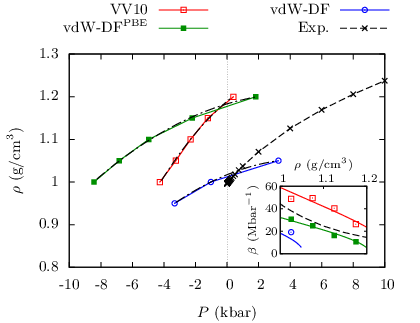

The calculated – equations of state for VV10 and vdW-DFPBE are shown in Fig. 4, alongside previous results for vdW-DF (with revPBE exchange). We perform a series of AIMD simulations at fixed densities between 1.00 and 1.20 g/cm3, in steps of 0.05 g/cm3, and we fit to a virial equation in powers of , up to second order. The excellent fits indicate the small uncertainty of our average pressures. This is also shown in Fig. 5: the cumulative running average for the instantaneous pressure stays almost constant after the first 10 ps of the simulation. We have carried out the same simulations for vdW-DFPBE with a smaller cell of 128 molecules. The pressure difference between the two sizes is small (0.6 kbar RMS), confirming that we are well converged in system size, in agreement with previous tests performed with the TIP4P force field [28]. However, the error bars are noticeably larger for the smaller system, leading to a worse fit for .
As shown by Wang et al. [28], the original vdW-DF functional gives the best density of liquid water at ambient pressure (1.00 g/cm3 at 0.0 kbar), perfectly correcting for the low densities given by all GGA functionals. However, it severely underestimates the compressibility, suggesting that the agreement at ambient pressure is fortuitous. This is confirmed by its RDF at 1.00 g/cm3, which is in much poorer agreement with experiment than even those obtained using GGA.
| Exp. [49] | VV10 (error) | vdW-DFPBE (error) | vdW-DF [28] (error) | |
|---|---|---|---|---|
| ( g/cm3) (Mbar-1) | 45.0 | 59.0 (+31%) | 32.2 (28%) | 18.2 (60%) |
| ( kbar) (Mbar-1) | 25.8 (43%) | 09.4 (79%) | 14.8 (67%) |
In contrast, our results show that VV10 and vdW-DFPBE reproduce the overall shape of the equation of state much better, despite a shift towards negative pressures that results in an equilibrium ambient density overestimated by almost 20% in both cases. Our results for the compressibility are given in Table 1 and in the inset of Fig. 4. The experimental value is between those of VV10 and vdW-DFPBE over the entire density range, with discrepancies of 30% at 1.00 g/cm3, while vdW-DF greatly underestimates it.
It is interesting to compare these results with those reported by Pi et al. [4] for four popular force-field models, all of which overestimate the compressibility at ambient density, with errors ranging from 26.7% (for TIP5P [50]) down to only 2.4% for SPC/E [51] and 2.9% for TIP4P/2005 [3]. However, when examining the change in compressibility with temperature, it is clear that only one model, TIP4P/2005, correctly reproduces the experimental data for a wide range of temperatures (including the existence of a minimum at 320 K), while the small error at ambient temperature for SPC/E can be seen to be fortuitous. Furthermore, TIP5P does not show any sign of the anomalous behaviour in the range considered. It is encouraging to note that, when analysing our results for vdW-DFPBE with 128 molecules at two different temperatures (260 K and 300 K, as listed in Appendix A) with the best fit through the data points, we find an increase in the compressibility at 1.00 g/cm3 of 20% for the low temperature simulations respect to the ambient temperature ones, in reasonable agreement with experiment [4] (27.6%), and better than TIP4P/2005 (11.0%). It seems likely, therefore, that vdW-DFPBE will also exhibit the compressibility anomaly.
III.2 Structural variations with density


The RDFs of VV10 and vdW-DFPBE are compared with a recent determination from x-ray diffraction [52] at ambient conditions (the lowest density line in Fig. 6). VV10 is overstructured, but with excellent agreement in the position of the extrema, while vdW-DFPBE is only slightly understructured, with a small outwards shift of 0.1 Å for the first maximum and a larger inwards shift of 0.3 Å for the second one. As explained by Wang et al., vdW-DFPBE corrects the low density of the GGA liquid by favoring the population of the anti-tetrahedral interstitial sites of the H-bond network, at the cost of breaking some H bonds. This results in a significantly different RDF for vdW-DFPBE respect to its underlying PBE functional (lower panel of Fig. 7). These anti-tetrahedral interstitial sites correspond to vdW-induced local minima in non-H-bonded dimer configurations.
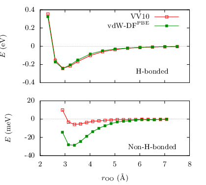
We have compared the energetics of H-bonded and non-H-bonded configurations for VV10 and vdW-DFPBE (Fig. 8). While the H-bonded binding energy is almost identical for both functionals (247 meV for VV10 and 245 meV for vdW-DFPBE), the non-H-bonded one is almost five times stronger in vdW-DFPBE (29 meV) than in VV10 (6 meV).
We have seen that the density of the VV10 liquid increases with respect to that of GGA functionals. In the upper panel of Fig. 7, we show the O–O RDFs for VV10 and PBEPW86R, the underlying semi-local functional used in VV10 (see Table 2), both at the same density of 1.00 g/cm3. Despite the two RDFs being very similar in this case, the corresponding pressures are very different (4.2 kbar and 3.5 kbar, respectively). Therefore, the reason why the density of VV10 water increases with respect to its underlying semi-local functional is due to a different mechanism to the one described above for vdW-DFPBE. While the topology of the H-bond network is not modified, there is an overall attraction between non-H-bonded molecules that reduces the pressure of the simulation. In vdW-DFPBE the non-H-bonded binding energy is so large that it favors the breaking of weak H bonds, modifying the structure of the H-bond network and favoring the positioning of molecules at anti-tetrahedral interstitial sites.

Fig. 6 also shows the change of the RDFs with increasing density, from 1.00 g/cm3 to 1.20 g/cm3 (see Appendix A for more details on the behavior of the extrema). Of these, Fig. 9 shows the lowest and highest densities only, decomposed in terms of the H-bond network (see Appendix B for a description of our H-bond definition). We see a different behavior for the two functionals. Although in both cases the liquid becomes less structured at higher density, for VV10 the second H-bonded shell moves inwards, closing the angle. For vdW-DFPBE the increase in pressure induces a larger population of the interstitial anti-tetrahedral sites, and the second H-bonded shell presents a bimodal behavior, some molecules moving inwards and some outwards (opening the angle).

These results can be compared with those reported by Soper and Ricci [53] for neutron diffraction of cold water under pressure. They assume that the measured structure factors can be described as a linear combination of two components, corresponding to a low- and a high-density liquid (LDL and HDL, respectively). Fitting their data to this model for a range of pressures, they extrapolate to obtain the pure LDL and HDL structures and densities at 268 K. We have simulated 128 molecules at the predicted densities for LDL and HDL, at 260 K. Fig 10 compares the resulting ab initio RDFs with the experimentally extrapolated ones. There is a very good agreement between low-density VV10 and the predicted LDL, and a truly remarkable agreement between high-density vdW-DFPBE and the predicted HDL. In particular, vdW-DFPBE reproduces an extended minimum at Å due to the bimodal structure of the second H-bonded shell 11 1 Interestingly, a recent classical force-field simulation [68] of thin-film water on a BaF2 surface has reported a very similar extended minimum in the RDF for the first 1 Å-thick water layer above the surface, which is therefore suggested to be in a highly compressed state similar to HDL.. On the other hand, the two functionals show quite different features for the opposite limits: vdW-DFPBE is understructured at low density, while VV10 does not exhibit the correct structure at high density. Our findings, therefore, rationalize the discrepancies observed at intermediate densities, for which both functionals give too large a weight to one of the two components 22 2 The – curves in Fig. 4 arguably reveal the same behavior: by extrapolating the vdW-DFPBE curve, we can see a tentative crossing with experiment around 1.25 g/cm3 and, analogously, a crossing of VV10 with experiment at low density (the precise value being harder to estimate in this case)..

We now investigate this conclusion in more detail, by attempting a quantitative analysis based on the same linear mixing model employed by Soper and Ricci. The RDF at a given temperature and density (and for a given xc functional) is assumed to be a simple linear combination of the HDL and LDL RDFs extrapolated from experimental data, with weights of and , respectively. We neglect cross terms between the two RDFs [27], as well as any additional dependence of each individual RDF on temperature or pressure. For any particular RDF obtained by AIMD simulation, we can then find the ‘best fit’ value of by minimizing the quantity
| (2) |
where we take Å and Å (the first peak is excluded, since small variations in its width can result in large changes in height, thereby swamping the more relevant and reliable variations around the second peak). The results of this analysis are shown in Fig 11. The previously postulated behavior of the two functionals can now be seen very clearly: vdW-DFPBE accurately recovers the HDL structure at high density, while VV10 fairly accurately recovers the LDL one at low density. However, in both cases the rate of change of with density is too small, resulting in each functional giving too much weight to its preferred structure at the opposite limit, as well as in between (e.g., at ambient density). We note that we find for vdW-DFPBE at ambient temperature and high density; this is a possible indication that the extrapolated end-point structures are themselves not pure HDL or LDL, but still contain a small amount of mixing.
It is interesting to note that our results confirm the suggestion of Møgelhøj et al. [27] of the similarity of the RDF obtained using a semi-local functional (PBE) with the LDL structure, and of those obtained using two non-local functionals (optPBE-vdW [23] and vdW-DF2 [24]) with the HDL structure. Their simulations are performed at ambient temperature and density, and, indeed, we find a good agreement between the RDF for PBE and that for VV10 (also at ambient temperature and density), and a fairly good agreement between the RDFs for the two non-local functionals and that for vdW-DFPBE. As we have discussed, VV10 barely modifies the RDF of its underlying semi-local functional, hence the similarity with PBE as well. The similarity between vdW-DFPBE, optPBE-vdW, and vdW-DF2 is also not surprising, as they are all related to the vdW-DF functional of Dion et al. [22], with some modifications in each case that improve the H-bond description. However, the latter two are even more severely understructured than vdW-DFPBE at ambient conditions (this discrepancy is reduced but not eliminated by accounting for finite size effects, shown in Fig. 1 for vdW-DFPBE).
III.3 Diffusivity
Finally, we show that our simulations allow us to evaluate one of the anomalies of the liquid. The experimental self-diffusion coefficient increases with density (or pressure) up to a maximum at 1.03 g/cm3 (at 300 K), above which the expected decrease is observed [56, 57]. This anomaly has been thoroughly studied and is well reproduced by empirical force fields [58, 59, 60]. However, first principles calculations of are especially challenging due to the relatively small system sizes and simulation times accessible with AIMD [18, 19]; in particular, system size effects are much larger for dynamical properties than for structural ones [61, 39].
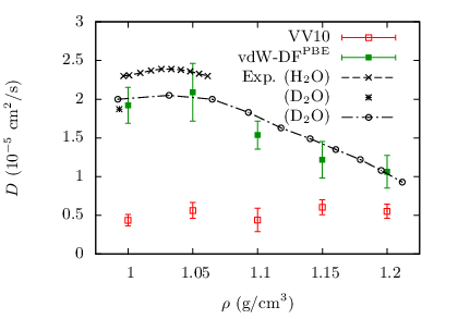
Our large 200-molecule simulation box and reasonably long AIMD runs have reduced the uncertainty enough to observe a clear trend in , as shown in Fig. 12. The finite size correction proposed by Dünweg and Kremer [61] (not included) is fairly small for our system size: an increase of cm2/s using the parametrization calculated by Kühne et al. for PBE [39].
We find vdW-DFPBE to be extremely successful, perfectly reproducing NMR spin-echo measurements [62] within the statistical errors. Furthermore, within our density resolution, shows a maximum at 1.05 g/cm3, in agreement with experiment. However, this result must be carefully assessed, as the density point giving the diffusivity maximum equilibrated to a temperature 10 K higher than the two points around it. This suggests that it might only be an apparent maximum, caused by the increased temperature at that point (in fact, this is also reflected in the large error bars). Indeed, experimental results show that an increase of 10 K in temperature can cause an increase of 0.5–0.6 g/cm3 in the self-diffusion coefficient both for light and heavy water [56, 57, 62]. On the other hand, it also possible that the diffusivity of the liquid is mostly determined by the original temperature (and the corresponding structure) at which the system was equilibrated (300 K for all points), rather than the average temperature reached during the NVE simulation. In favor of this latter hypothesis, we note that the simulations at 1.15 g/cm3 and 1.20 g/cm3 also featured a similar increase in temperature; however, applying an approximate correction only to these three points results in a less smooth trend overall, with a minimum at 1.05 g/cm3 and a maximum at 1.10 g/cm3. Furthermore, using this correction, the only points to maintain a good agreement with the experimental curve would be those at 1.00 g/cm3 and 1.10 g/cm3 (i.e., the uncorrected ones). It seems quite unlikely that, while these two points do indeed agree with experiment, the equally good agreement of the other three points shown in Fig. 12 is merely fortuitous.
In contrast to these promising results, VV10 shows a nearly density-independent and significantly underestimated diffusivity (by 78% at 1.00 g/cm3, similarly to previous GGA results [18]). This is directly related to an overstructured liquid [18, 19]: for all the densities considered, indicates that the system is effectively supercooled, with too strong a H-bond network.
IV Conclusions
We have performed a detailed study of first principles models of liquid water with DFT, using two non-local density functionals that describe vdW interactions without empirical parameters. We have calculated the – equation of state at room temperature, from which we extract the equilibrium ambient density and the compressibility, structural properties given by the O–O RDF, and the diffusivity as a function of density.
For these properties, we find that the vdW-DF functional, with PBE exchange, arguably gives the better description of the liquid. In particular, the self-diffusion coefficient is in excellent agreement with experiments and it appears to correctly reproduce the isothermal anomaly, within the error margins of the AIMD simulations. The differences between xc functionals also provide valuable insights. Interestingly, vdW-DFPBE and VV10 seem to complement each other, by describing respectively the high- and low-density structures of water with remarkable precision. Thus, to reach a better description of the liquid, new functionals should improve the energy landscape between these two structures.
Acknowledgements.
This work was partly funded by grants FIS2009-12721 and FIS2012-37549 from the Spanish Ministry of Science. MVFS acknowledges a DOE Early Career Award No. DE-SC0003871. The calculations were performed on the following HPC clusters: kroketa (CIC nanoGUNE, Spain), arina (Universidad del País Vasco/Euskal Herriko Unibertsitatea, Spain), magerit (CeSViMa, Universidad Politécnica de Madrid, Spain). We thank the RES–Red Española de Supercomputación for access to magerit. SGIker (UPV/EHU, MICINN, GV/EJ, ERDF and ESF) support is gratefully acknowledged.Appendix A Overview of simulations
| vdW-DF | vdW-DFPBE | PBEPW86R | VV10 | VV10revPBE | |
|---|---|---|---|---|---|
| revPBE [43] | PBE [44] | PW86R [45] | PW86R | revPBE | |
| LDA [63] | LDA | PBE | PBE | PBE | |
| vdW-DF [22] | vdW-DF | - | VV10 [25] | VV10 |
| () | () | RDF extrema ( (Å), ) | ||||||||
| (ps) | () | (K) | (kbar) | ( /s) | 1st max. | 1st min. | 2nd max. | 2nd min. | ||
| 64 | vdW-DFPBE | 10.0 | 1.00 | 308 (300) | 8.5 (8.6) | 2.1 | ||||
| vdW-DF | 10.0 | 1.00 | 308 (300) | 0.7 (0.9) | 3.3 | - | - | |||
| 128 | vdW-DFPBE | 10.0 | 1.20 | 301 (300) | 1.1 (1.1) | 0.9 | - | - | ||
| 10.0 | 1.15 | 316 (300) | 1.3 (1.1) | 1.3 | - | - | ||||
| 10.0 | 1.10 | 309 (300) | 4.8 (4.8) | 1.5 | - | - | ||||
| 10.0 | 1.05 | 304 (300) | 6.9 (6.9) | 1.2 | ||||||
| 10.0 | 1.00 | 301 (300) | 8.3 (8.3) | 1.7 | ||||||
| 10.0 | 0.88 | 312 (300) | 7.0 (7.1) | 2.6 | ||||||
| 10.0 | 1.20 | 265 (260) | 0.4 (0.3) | 0.5 | - | - | ||||
| 10.0 | 1.15 | 263 (260) | 3.4 (3.4) | 0.4 | ||||||
| 10.0 | 1.10 | 264 (260) | 5.6 (5.6) | 0.6 | ||||||
| 10.0 | 1.05 | 264 (260) | 8.1 (8.1) | 0.5 | ||||||
| 10.0 | 1.00 | 262 (260) | 8.9 (9.0) | 0.6 | ||||||
| 10.0 | 0.88 | 265 (260) | 9.1 (9.3) | 0.8 | ||||||
| vdW-DFPBE | 02.5 | 1.00 | 289 (300) | 5.2 (5.0) | 1.9 | |||||
| () | ||||||||||
| PBEPW86R | 10.0 | 1.00 | 307 (300) | 3.8 (3.5) | 0.8 | |||||
| VV10 | 10.0 | 1.20 | 262 (260) | 0.6 (0.5) | 0.3 | |||||
| 10.0 | 0.88 | 267 (260) | 5.8 (6.1) | 0.2 | ||||||
| VV10revPBE | 10.0 | 1.00 | 300 (300) | 1.5 (1.5) | 0.8 | |||||
| 200 | vdW-DFPBE | 20.0 | 1.20 | 308 (300) | 1.7 (1.8) | 1.1 | - | - | ||
| 20.0 | 1.15 | 307 (300) | 2.3 (2.2) | 1.2 | - | - | ||||
| 20.0 | 1.10 | 301 (300) | 5.0 (5.0) | 1.5 | - | - | ||||
| 20.0 | 1.05 | 312 (300) | 6.8 (6.8) | 2.1 | ||||||
| 20.0 | 1.00 | 301 (300) | 8.4 (8.4) | 1.9 | ||||||
| VV10 | 20.0 | 1.20 | 304 (300) | 0.5 (0.4) | 0.6 | |||||
| 20.0 | 1.15 | 308 (300) | 0.8 (1.2) | 0.6 | ||||||
| 20.0 | 1.10 | 311 (300) | 2.2 (2.3) | 0.4 | ||||||
| 20.0 | 1.05 | 311 (300) | 3.1 (3.2) | 0.6 | ||||||
| 20.0 | 1.00 | 314 (300) | 3.4 (4.2) | 0.4 | ||||||
| Exp. [49, 57, 56, 52] | 1.00 | 300 | 0.0 | 2.3 (H2O) | ||||||
| 1.9 (D2O) | ||||||||||
We have performed AIMD simulations at three different system sizes (64, 128 and 200 molecules), and using five different xc functionals (listed in Table 2). Table 3 details all these simulations, including both the input parameters and the post-processing results. Unless otherwise stated, we use the basis.


Fig. 13 shows the comparison of the RDFs from AIMD simulations with experiment for four different xc functionals. All simulations are performed at the same density and temperature, although with differing system sizes (see Table 3). The experimental data from x-ray diffraction measurements [52] is for ambient conditions.


Finally, Fig. 14 shows how the radial position and height of the first three maxima and minima in the RDF change with density at 300 K for VV10 and vdW-DFPBE.
Appendix B H-bond definition
We describe here our criterion for the existence of a H bond between two molecules, used in the RDF decomposition of Fig. 9, as well as previously in Wang et al. [28].
In the standard geometrical definition, a H bond exists if two conditions are satisfied: (i) the intermolecular distance , where is usually chosen as the position of the first minimum in the O–O RDF (3.5 Å), and (ii) the angle , where indicate the acceptor or donor character of the molecules participating in the bond, and is a cutoff angle. However, this definition ignores the electronic distribution of the acceptor molecule, which plays an essential role in H bonds [64, 65].
We consider a donor H atom and an acceptor lone pair (L), and we define that a H bond exists if their distance Å. The lone pair centers can be obtained from their maximally localized Wannier orbitals [66], but the cost of this calculation at every time step would be prohibitive. Instead, assuming that the two bonding orbitals are in the OH directions, we use the orthogonality of the four hybrid orbitals to determine the angle between the lone pair directions:
| (3) |
Then, the positions of the two lone pair centers are
| (4) |
where and are unit vectors along the HOH bisector and normal to the molecular plane, respectively, and is the distance of the lone pair centers to the oxygen atom. We use the value of the TIP5P model [50] ( Å) which is very close to that of the ST2 model [67] (0.8 Å). Although this is about two times longer than the distance of Wannier orbitals, we have found that the H-bond definition is very insensitive to and , provided that Å. We have also checked that this definition produces very similar results to those of an electronic-based criterion, such as the Mulliken overlap [64].
Appendix C Static and dynamic pressure differences
| PBE | revPBE | PBEPW86R | vdW-DF | vdW-DFPBE | VV10 | |||||||||||||
|---|---|---|---|---|---|---|---|---|---|---|---|---|---|---|---|---|---|---|
| PBE | - | |||||||||||||||||
| revPBE | 7.8 | 7.3 | 0.5 | - | ||||||||||||||
| PBEPW86R | 0.3 | 1.1 | 1.4 | 7.5 | 6.2 | 1.3 | - | |||||||||||
| vdW-DF | 2.3 | 1.4 | 3.7 | 10.1 | 5.9 | 4.2 | 2.6 | 0.3 | 2.9 | - | ||||||||
| vdW-DFPBE | 11.7 | 6.0 | 5.7 | 19.5 | 13.3 | 6.2 | 11.9 | 7.1 | 4.8 | 9.4 | 7.4 | 2.0 | - | |||||
| VV10 | 7.5 | 6.2 | 1.3 | 15.3 | 13.5 | 1.8 | 7.8 | 7.3 | 0.5 | 5.2 | 7.6 | 2.4 | 4.2 | 0.2 | 4.4 | - | ||
| VV10PBE | 1.7 | 0.3 | 1.4 | 9.5 | 7.0 | 2.5 | 2.0 | 0.8 | 1.2 | 0.6 | 1.1 | 0.5 | 10.0 | 6.3 | 3.7 | 5.8 | 6.4 | 0.6 |
In order to investigate the variation in average pressure in the AIMD simulations due to the xc functional, we have calculated ‘static’ and ‘dynamic’ contributions to the total pressure difference between pairs of functionals, listed in Table 4. We make use of three GGA functionals and four vdW functionals (two based on vdW-DF, and two based on VV10).
The total difference is calculated using the average pressures obtained from the AIMD simulations (see Table 3). Instead, the static difference is obtained from the average pressures calculated using the same 200 snapshots of liquid water for both functionals. These include both low- and high-density configurations of the liquid. We find that there is an almost constant difference between functionals when calculating from the same snapshot. Finally, the dynamic difference is taken as the discrepancy between and . A large value of , therefore, indicates that the two functionals are exploring significantly different configurations during the AIMD simulation.
From the results presented in the table, we find that the largest values of are for differences between vdW-DF and GGA functionals (4.7 kbar RMS), followed by differences between vdW-DF and VV10 functionals (3.1 kbar RMS). Instead, differences between VV10 and GGA functionals are much smaller (1.6 kbar RMS), as well as those between different GGA functionals (1.1 kbar RMS). Therefore, this suggests that vdW-DF significantly alters the sampling of configuration space compared to GGA, while VV10 has only a small effect in this respect.
References
- [1] B. Guillot, J. Mol. Liq. 101, 219 (2002).
- [2] D. Paschek, J. Chem. Phys. 120, 6674 (2004).
- [3] J. L. F. Abascal and C. Vega, J. Chem. Phys. 123, 234505 (2005).
- [4] H. L. Pi, J. L. Aragones, C. Vega, E. G. Noya, J. L. F. Abascal, M. A. Gonzalez, and C. McBride, Mol. Phys. 107, 365 (2009).
- [5] F. Sciortino, P. H. Poole, U. Essmann, and H. E. Stanley, Phys. Rev. E 55, 727 (1997).
- [6] E. B. Moore and V. Molinero, Nature 479, 506 (2011).
- [7] D. T. Limmer and D. Chandler, J. Chem. Phys. 137, 044509 (2012).
- [8] F. Mallamace, C. Corsaro, and H. E. Stanley, Proc. Natl. Acad. Sci. USA 110, 4899 (2013).
- [9] C. Huang, K. T. Wikfeldt, T. Tokushima, D. Nordlund, Y. Harada, U. Bergmann, M. Niebuhr, T. M. Weiss, Y. Horikawa, M. Leetmaa, M. P. Ljungberg, O. Takahashi, A. Lenz, L. Ojamäe, A. P. Lyubartsev, S. Shin, L. G. M. Pettersson, and A. Nilsson, Proc. Natl. Acad. Sci. USA 106, 15214 (2009).
- [10] P. Kumar and H. E. Stanley, J. Phys. Chem. B 115, 14269 (2011).
- [11] F. Sciortino, I. Saika-Voivod, and P. H. Poole, Phys. Chem. Chem. Phys. 13, 19759 (2011).
- [12] J. L. F. Abascal and C. Vega, J. Chem. Phys. 134, 186101 (2011).
- [13] D. Paschek, Phys. Rev. Lett. 94, 217802 (2005).
- [14] D. Corradini, M. Rovere, and P. Gallo, J. Chem. Phys. 132, 134508 (2010).
- [15] J. L. F. Abascal and C. Vega, J. Chem. Phys. 133, 234502 (2010).
- [16] B. Pamuk, J. M. Soler, R. Ramírez, C. P. Herrero, P. W. Stephens, P. B. Allen, and M.-V. Fernández-Serra, Phys. Rev. Lett. 108, 193003 (2012).
- [17] J. C. Grossman, E. Schwegler, E. W. Draeger, F. Gygi, and G. Galli, J. Chem. Phys. 120, 300 (2004).
- [18] M.-V. Fernández-Serra and E. Artacho, J. Chem. Phys. 121, 11136 (2004).
- [19] I.-F. W. Kuo, C. J. Mundy, M. J. McGrath, J. I. Siepmann, J. VandeVondele, M. Sprik, J. Hutter, B. Chen, M. L. Klein, F. Mohamed, M. Krack, and M. Parrinello, J. Phys. Chem. B 108, 12990 (2004).
- [20] P. H.-L. Sit and N. Marzari, J. Chem. Phys. 122, 204510 (2005).
- [21] J. Schmidt, J. VandeVondele, I.-F. W. Kuo, D. Sebastiani, J. I. Siepmann, J. Hutter, and C. J. Mundy, J. Phys. Chem. B 113, 11959 (2009).
- [22] M. Dion, H. Rydberg, E. Schröder, D. C. Langreth, and B. I. Lundqvist, Phys. Rev. Lett. 92, 246401 (2004).
- [23] J. Klimes, D. R. Bowler, and A. Michaelides, J. Phys.: Condens. Matter 22, 022201 (2010).
- [24] K. Lee, E. D. Murray, L. Kong, B. I. Lundqvist, and D. C. Langreth, Phys. Rev. B 82, 081101(R) (2010).
- [25] O. A. Vydrov and T. Van Voorhis, J. Chem. Phys. 133, 244103 (2010).
- [26] I.-C. Lin, A. P. Seitsonen, M. D. Coutinho-Neto, I. Tavernelli, and U. Rothlisberger, J. Phys. Chem. B 113, 1127 (2009).
- [27] A. Møgelhøj, A. K. Kelkkanen, K. T. Wikfeldt, J. Schiøtz, J. J. Mortensen, L. G. M. Pettersson, B. I. Lundqvist, K. W. Jacobsen, A. Nilsson, and J. K. Nørskov, J. Phys. Chem. B 115, 14149 (2011).
- [28] J. Wang, G. Román-Pérez, J. M. Soler, E. Artacho, and M.-V. Fernández-Serra, J. Chem. Phys. 134, 024516 (2011).
- [29] C. Zhang, J. Wu, G. Galli, and F. Gygi, J. Chem. Theory Comput. 7, 3054 (2011).
- [30] K. T. Wikfeldt, A. Nilsson, and L. G. M. Pettersson, Phys. Chem. Chem. Phys. 13, 19918 (2011).
- [31] E. D. Murray and G. Galli, Phys. Rev. Lett. 108, 105502 (2012).
- [32] J. M. Soler, E. Artacho, J. D. Gale, A. García, J. Junquera, P. Ordejón, and D. Sánchez-Portal, J. Phys.: Condens. Matter 14, 2745 (2002).
- [33] N. Troullier and J. L. Martins, Phys. Rev. B 43, 1993 (1991).
- [34] J. Junquera, O. Paz, D. Sánchez-Portal, and E. Artacho, Phys. Rev. B 64, 235111 (2001).
- [35] E. Anglada, J. M. Soler, J. Junquera, and E. Artacho, Phys. Rev. B 66, 205101 (2002).
- [36] F. Corsetti, M.-V. Fernández-Serra, J. M. Soler, and E. Artacho, J. Phys.: Condens. Matter 25, 435504 (2013).
- [37] W. L. Jorgensen, J. Chandrasekhar, J. D. Madura, R. W. Impey, and M. L. Klein, J. Chem. Phys. 79, 926 (1983).
- [38] H. J. C. Berendsen, D. van der Spoel, and R. van Drunen, Comput. Phys. Commun. 91, 43 (1995).
- [39] T. D. Kühne, M. Krack, and M. Parrinello, J. Chem. Theory Comput. 5, 235 (2009).
- [40] X. Gonze et al., Comput. Phys. Commun. 180, 2582 (2009).
- [41] L. Kleinman and D. M. Bylander, Phys. Rev. Lett. 48, 1425 (1982).
- [42] R. D. Meade and D. Vanderbilt, Mat. Res. Soc. Symp. Proc. 141, 451 (1989).
- [43] Y. Zhang and W. Yang, J. Chem. Phys. 80, 890 (1998).
- [44] J. P. Perdew, K. Burke, and M. Ernzerhof, Phys. Rev. Lett. 77, 3865 (1996).
- [45] É. D. Murray, K. Lee, and D. C. Langreth, J. Chem. Theory Comput. 5, 2754 (2009).
- [46] G. Román-Pérez and J. M. Soler, Phys. Rev. Lett. 103, 096102 (2009).
- [47] R. Sabatini, T. Gorni, and S. de Gironcoli, Phys. Rev. B 87, 041108(R) (2013).
- [48] J. Wu and F. Gygi, J. Chem. Phys. 136, 224107 (2012).
- [49] W. Wagner and A. Pruß, J. Phys. Chem. Ref. Data 31, 387 (2002).
- [50] M. W. Mahoney and W. L. Jorgensen, J. Chem. Phys. 112, 8910 (2000).
- [51] H. J. C. Berendsen, J. R. Grigera, and T. P. Straatsma, J. Phys. Chem. 91, 6269 (1987).
- [52] L. B. Skinner, C. Huang, D. Schlesinger, L. G. M. Pettersson, A. Nilsson, and C. J. Benmore, J. Chem. Phys. 138, 074506 (2013).
- [53] A. K. Soper and M. A. Ricci, Phys. Rev. Lett. 84, 2881 (2000).
- [54] Interestingly, a recent classical force-field simulation [68] of thin-film water on a BaF2 surface has reported a very similar extended minimum in the RDF for the first 1 Å-thick water layer above the surface, which is therefore suggested to be in a highly compressed state similar to HDL.
- [55] The – curves in Fig. 4 arguably reveal the same behavior: by extrapolating the vdW-DFPBE curve, we can see a tentative crossing with experiment around 1.25 g/cm3 and, analogously, a crossing of VV10 with experiment at low density (the precise value being harder to estimate in this case).
- [56] K. Krynicki, C. D. Green, and D. W. Sawyer, Faraday Discuss. Chem. Soc. 66, 199 (1978).
- [57] R. Mills, J. Phys. Chem. 77, 685 (1973).
- [58] A. Scala, F. W. Starr, E. La Nave, F. Sciortino, and H. E. Stanley, Nature 406, 166 (2000).
- [59] J. R. Errington and P. G. Debenedetti, Nature 409, 318 (2001).
- [60] P. A. Netz, F. Starr, M. C. Barbosa, and H. E. Stanley, J. Mol. Liq. 101, 159 (2002).
- [61] B. Dünweg and K. Kremer, J. Chem. Phys. 99, 6983 (1993).
- [62] D. J. Wilbur, T. DeFries, and J. Jonas, J. Chem. Phys. 65, 1783 (1976).
- [63] J. P. Perdew and A. Zunger, Phys. Rev. B 23, 5048 (1981).
- [64] M. V. Fernández-Serra and E. Artacho, Phys. Rev. Lett. 96, 016404 (2006).
- [65] R. Kumar, J. R. Schmidt, and J. L. Skinner, J. Chem. Phys. 126, 204107 (2007).
- [66] M. Sharma, R. Resta, and R. Car, Phys. Rev. Lett. 95, 187401 (2005).
- [67] F. H. Stillinger and A. Rahman, J. Chem. Phys. 60, 1545 (1974).
- [68] S. Kaya, D. Schlesinger, S. Yamamoto, J. T. Newberg, H. Bluhm, H. Ogasawara, T. Kendelewicz, G. E. Brown Jr., L. G. M. Pettersson, and A. Nilsson, Sci. Rep. 3, 1074 (2013).