Determination of hydrogen cluster velocities and comparison with numerical calculations
Abstract
The use of powerful hydrogen cluster jet targets in storage ring experiments led to the need of precise data on the mean cluster velocity as function of the stagnation temperature and pressure for the determination of the volume density of the target beams. For this purpose a large data set of hydrogen cluster velocity distributions and mean velocities was measured at a high density hydrogen cluster jet target using a trumpet shaped nozzle. The measurements have been performed at pressures above and below the critical pressure and for a broad range of temperatures relevant for target operation, e.g., at storage ring experiments. The used experimental method is described which allows for the velocity measurement of single clusters using a time-of-flight technique. Since this method is rather time-consuming and these measurements are typically interfering negatively with storage ring experiments, a method for a precise calculation of these mean velocities was needed. For this, the determined mean cluster velocities are compared with model calculations based on an isentropic one-dimensional van der Waals gas. Based on the obtained data and the presented numerical calculations, a new method has been developed which allows to predict the mean cluster velocities with an accuracy of about 5%. For this two cut-off parameters defining positions inside the nozzle are introduced, which can be determined for a given nozzle by only two velocity measurements.
Keywords:
hydrogen; molecular clusters; velocity; time-of-flight method; Laval nozzlepacs
47.40.Ki, 05.70.Ce, 36.40.-cI Introduction
Cluster beams have been studied in the last century extensively with respect to their physical and chemical properties and even today the interest in technological applications is increasing rapidly[1]. Prominent examples are the use for cluster beam deposition, cluster impact lithography, and the application as target beams in, e.g., storage ring experiments which has started only in the last few decades. For applications in hadron physics experiments or in experiments with high intense laser beams, the most important advantage is that they provide a pure target material inside a vacuum chamber with densities in the range between gas beams and the solid state targets. Cluster beams consisting of particles with sizes from the nanometer to the micrometer scale propagate through vacuum with almost no increase of their angular spread, so that it is possible to provide a spatially well defined interaction zone for, e.g., a particle beam in a storage ring or a laser beam.
In hadron physics experiments at a storage ring the cluster beams are typically produced by expansion of gaseous materials in Laval type nozzles. Although such targets can be operated in principal with all kind of gaseous materials ranging from hydrogen to, e.g., xenon, the use of hydrogen is of special interest as effective proton target for the investigation of elementary reactions. Examples for experimental facilities using such hydrogen cluster beams as internal targets at a storage ring are the ANKE[2] experiment and the former COSY-11[3] experiment, both situated at the COSY[4] accelerator of the Forschungszentrum Jülich. For the established internal target experiments mainly the density and the purity of the cluster beams were important, but for the design of new experimental facilities which can be operated with event rates increased by one or two orders of magnitude, the precise knowledge of microscopic properties, like velocity or mass distributions, or time structure, became of high importance. This information is especially important for the simulation of the interaction between intense pulsed laser beams and cluster beams. An example for a future experiment at a storage ring is the detector PANDA[5] at the planned accelerator centrum FAIR in Darmstadt (Germany). For this experiment a cluster jet target has been developed at the University of Münster where the number of target atoms per unit area is above at a distance of from the nozzle. A detailed description of this prototype is presented in Ref. 6 and Ref. 7. The measurements presented in this work have been performed at this prototype.
In these targets the clusters are produced from ultra-clean cold compressed hydrogen fluid with temperatures of, e.g., and pressures of about , which is pressed through a Laval nozzle with a minimum diameter in the order of . During the expansion of the fluid through the nozzle into a first vacuum chamber clusters are produced. Directly behind the nozzle the shape of the jet beam, consisting of both clusters and a gas beam, is determined by the shape of the divergent part of the production nozzle. In order to prepare a well defined cluster beam for experiments and to suppress the disturbing residual gas background from the gas beam, a set of two skimmers is used to separate differential pumping stages. The second skimmer, which is denoted in the following as collimator, determines the final shape and size of the cluster beam at all further vacuum stages, and especially at the interaction point with the beam of the storage ring in the scattering chamber. For more details see Ref. 6. A schematic sketch of this setup operated with gaseous hydrogen is shown in Fig. 1.

For an optimized use as internal target in storage ring experiments, e.g., for hadron physics experiments, it is essential to determine and to adjust the target thickness , the number of target atoms per unit area. With the knowledge of the thickness the luminosity of the internal experiment can be calculated (see, e.g., Ref. 8), where is the revolution frequency and the number of circulating particles in the storage ring. Given the cross section of a specific reaction between target and storage ring beam particles, the mean rate of these reactions can be determined. This determination is especially important for adjusting the target thickness to achieve a desired reaction rate and to estimate the rate of background events. Using a Cartesian coordinate system, where the cluster beam propagates along the z axis and the stored beam along the x axis and assuming that the transverse width of the stored beam is negligible compared to the size of the cluster beam, it is possible to calculate the target thickness in units of number of atoms per square centimeter at a specific distance behind the nozzle directly from the volume density distribution [6]:
| (1) |
where is the molar mass of the gas atoms and the Avogadro constant. In case of the cluster jet target the thickness can be measured by inserting movable rods into the cluster jet. At the cluster target prototype for the PANDA experiment such rods are mounted in a scattering chamber located approximately two meters behind the nozzle (Fig. 2). Here the rod diameter of is small compared to the size of the cluster jet which is typically in the order of about . Clusters colliding with these rods are stopped and lead by evaporation to an increase of the vacuum pressure in this chamber. In Fig. 3 a typical measurement of the vacuum pressure is presented, where the pressure increase is plotted as a function of the rod position. With such kind of measurements the size as well as the position of the cluster jet within the vacuum stage can be determined easily. Moreover, assuming a specific volume density distribution this pressure profile can be described by the following equation [6]:
| (2) |


In this equation is the background pressure, the center position of the cluster jet, the universal gas constant, the molar mass of the gas, the known pumping speed of the used pumping system, and the mean velocity of the clusters. Note that the velocity depends on the stagnation condition, i.e., the temperature and the pressure , as well as on the nozzle geometry. However, for constant numbers for and the velocity is constant. Therefore, in order to calculate the target thickness in a first step the target density distribution has to be adjusted to describe the relative shape of the measured pressure profile. For an absolute target density determination the mean velocity has to be known. In order to minimize the uncertainty of the extracted volume density, the mean velocity has to be measured with an accuracy which does not exceed the uncertainty of the pressure and of the pumping speed. At the presented setup both uncertainties amount to about 10%.
Since the cluster beams from the described cluster target sources are optimized for highest volume densities, the used nozzles differ significantly both in shape and size from the ones commonly used by groups specialized in the investigation of velocity and mass distributions, e.g., work on hydrogen clusters reported in Ref. 9. In the cited work a pin hole nozzle with a minimum diameter of was used, whereas for the production of the cluster beams described here trumped shaped nozzle geometries with minimum diameters of about are used. Both factors can significantly change the velocity distribution of the clusters in the generated beam and therefore new systematic studies of these cluster target beams had to be performed.
The mean velocity of the hydrogen clusters produced with a similar trumped shaped nozzle with a throat diameter of was already measured[10] at the target for the E835 experiment at FERMILAB and it was found, that it can be described adequately by the maximum local velocity of a perfect gas accelerated in an isentropic expansion through a convergent-divergent nozzle[10, 11]:
| (3) |
In this equation is the gas temperature at the inlet of the nozzle and is the adiabatic index. These measurements were done at a pressure below and temperatures between and where the hydrogen is in the gas phase before entering the nozzle. However, later optimization studies on hydrogen cluster targets[12, 6] showed that a significant performance increase is possible, i.e., an increase of the achievable maximum target thickness by orders of magnitude. One prerequisite for this is that the target is operated with hydrogen being in the liquid phase before entering the nozzle. Since it is known from previous measurements, e.g., Ref. 9, that the phase transition from the gas phase into the liquid phase has a significant impact on the cluster velocity, precise measurements on the velocity distributions and mean velocities as well as a comparison with the situation obtained with hydrogen being in the gas phase before entering the nozzle were strongly needed. Based on this data verifications and optimizations of calculations will be possible.
For this reason a dedicated time-of-flight system was designed and installed at the Münster cluster jet target. Detailed studies on the velocity distributions as function of the operating parameters were performed which is presented in the first part of this work.
Although the time-of-flight system enabled for a precise determination of the velocity distributions and with this for the calculation of the mean velocities, the measurement time of several hours makes it impractical to use this system regularly for the volume density determination described above. This is especially true for optimization studies where the temperature and pressure at the nozzle inlet is changed very often. Therefore it was essential to be able to calculate the mean cluster velocity as function of the stagnation conditions in the typical operation region with a precision, as discussed before, below 10%. Many groups, e.g., Ref. 9, Ref. 13, and Ref. 14 have measured mean velocities of clusters and extracted fluid properties like the temperature of the cluster at the end of the expansion based on different equations of state. Ref. 15, for example, used an equation of state to produce a theoretical prediction for the mean velocity by assuming a constant final temperature. The values predicted with this method deviate from the measurements presented in the same work by about 20%–40% for the data points measured at temperatures below the boiling point. Therefore a new method had to be developed to allow for more accurate predictions at the discussed stagnation conditions. In the second part of this work such a method is presented, introducing two parameters which had to be determined only once by a fit to the measured data. In the operation region of the investigated cluster source this techniques provides precise predictions with an average absolute deviation of only about 5% compared to the measured mean cluster velocities. This applies both to the regions of liquid and of gaseous hydrogen in front of the nozzle.
II Experimental setup

In Fig. 4 the schematic view of the utilized time-of-flight setup is shown. Clusters produced in the cluster source are ionized by a pulsed electron gun mounted at a short distance behind the collimator. This electron gun is operated in a pulsed mode with a repetition rate of about and a pulse width of approximately . The current of the electron beam is reduced in such a way that for each pulse no more than a single ionized cluster is registered. The ionized clusters itself are detected by a Channeltron after a flight path of . Due to this long distance and pulse widths in the microsecond time scale, the observed time-of-flight times being in the range between and can be obtained with high resolution. The start and stop pulses are detected by a timer system based on a MC9S08QG8 micro controller by Freescale Semiconductor and the time difference is send to a computer. A detailed description of the used software for the micro controller can be found in Ref. 7.

In order to extract time-of-flight information with high resolution the complete setup has to be calibrated with respect to possible timing offsets introduced by the pulsed electron gun device and the cluster detection system. For this purpose the calibration source for ions with known kinetic energy is used (Fig. 5). The source consists of two coaxial cylinders. The outer cylinder is electrically grounded while the inner cylinder is connected to a voltage source providing a potential of up to . The calibration source is mounted in such a way, that the cylinder axis is perpendicular to the axis of the incoming cluster beam, so that the clusters can enter through a hole with a diameter of . In the inner cylinder the clusters are stopped by a wedge shaped plate, evaporate and are converted into hydrogen gas. This gas is ionized by the pulsed electron beam entering along the axis of the two cylinders. The potential difference between the cylinders accelerate the produced ions to a known kinetic energy while they are extracted through a hole along the cluster beam axis. The ions leaving this unit drift towards the detection system which consists of an array of a grounded entrance orifice followed by a Channeltron. Here the Channeltron input is set on a negative potential of relative to the entrance orifice. Thus, positively charged ions and, in the later cluster time-of-flight measurements, positively charged clusters are accelerated and cause detectable signals.

In Fig. 6 an example of a time-of-flight distribution is shown before timing calibration which was measured using the calibration source with an acceleration voltage of . In this distribution four peaks from different ion species are clearly visible. The peak with the lowest mean time-of-flight can be attributed to photons produced in the cluster source. Since their time-of-flight is approximately the measured flight time of is a direct measure of the timing offset caused by the electronics. The three other peaks correspond to different hydrogen ions, namely , , and . The time offset and the length of the flight path between the electron gun and the Channeltron could be extracted by measuring the mean time-of-flight for the different ions as function of the acceleration voltage. For these measurements the electron gun was operated at a repetition rate of about and a pulse duration of about . With this calibration setup a time resolution of about was reached which is predominantly given by the pulse duration of the electron gun.
III Velocity distributions of clusters
Using the presented time-of-flight setup the velocity distributions of hydrogen clusters produced in the Münster cluster jet target setup were measured[16] using a nozzle with a minimum diameter of . For these measurements the pulse duration of the electron gun was increased to , so that the time resolution increases to about which is still very precise compared to the measured standard deviation of the typical velocity destributions of the clusters of several hundred to thousand microseconds.


In Fig. 7 and 8 the measured distributions of the cluster velocity are shown. In the first figure a constant pressure of was used in front of the nozzle and for the second figure were applied. In both figures the distributions at different fluid temperatures from up to are displayed. The distributions are scaled in such a way that the total area of each spectrum is the same in the respective figure.
In case of Fig. 8 where the data at are shown the distributions above the boiling point of around are relatively sharp with a standard deviation of about and have a negative skew. At the phase transition between gas and liquid a double peak structure is visible with a narrow peak at higher mean velocity on top of a broad peak with a lower mean velocity. The inlayed graph shows the development of this structure in the temperature range between and . At a temperature of around the width of the smaller peak is around at a mean velocity of about whereas the broader peak has a standard deviation of about and a mean velocity of .
This double peak structure was also observed in earlier experiments of other groups, presented, e.g., in Ref. 9, 13, and 15, both with hydrogen and helium. The cited authors explain their observations with a different kind of cluster production for the respective peak. They expect that the narrow peak consists of clusters which were formed from a gas by condensation whereas the broad peak should consist of clusters formed from a liquid by fragmentation.
Below the double peak structure disappears which can be seen in the second inlayed graph showing the measured distribution in the temperature range between and . At a temperature of the width of the narrow peak has increased to about in combination with a further reduced mean velocity of , while the standard deviation of the broader peak has increased to at a mean velocity of about . At lower temperatures only the broader peak remains although the width of the peak decreases with a further reduction of the fluid temperature from at to at . The described behavior is similar at different other pressures in front of the nozzle as can be seen in Fig. 7.
IV Mean cluster velocities
As mentioned before, the precise knowledge of the mean cluster velocity is needed for the estimation of the volume density of the cluster beam. Since it is not feasible to measure this quantity for each possible stagnation condition within the operation region of the cluster target, a method is needed to predict these values with an accuracy below about 10%. In contrast to other publications, e.g., Ref. 9, the main focus lies here on the description of the mean cluster velocity of the complete velocity distribution which in our case can be directly calculated from the measured velocities of the single clusters. We therefore will not quote the mean velocity of the two peaks observed in the phase transition region separately. In our case, where these two peaks completely overlap there is also no model independent way to extract this information.
IV.1 Experimental results
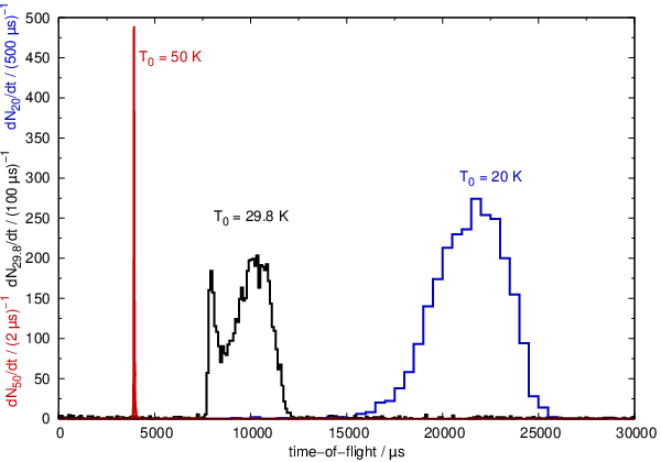

To summarize the above findings three examples for the measured time-of-flight distributions of hydrogen clusters are presented in Fig. 9. The distributions were measured at a constant hydrogen pressure of at the nozzle inlet, but at different temperatures of , , and . The distribution at highest temperature is very narrow with a standard deviation of which increases up to at . Near the boiling temperature of a double peak structure was observed with a small peak at higher velocity on top of a broad peak with a lower mean velocity indicating the different cluster production mechanism from the two coexisting phases. This dependance of the production process on the hydrogen phase state is also visible in Fig. 10 where the mean cluster velocity is plotted as function of the hydrogen temperature at the inlet of the nozzle at a constant inlet pressure of .
Above the boiling point the data can be described adequately by the maximum gas velocity of a perfect gas (Eq. (3)), which agrees well with the observations presented in Ref. 10 taken at lower inlet pressure of below . However, the data below the boiling point deviate from the calculated ones by up to a factor of three, which is in agreement with the results presented in Ref. 9.
A collection of measured mean velocities for different isobars is presented in Fig. 11. Since the boiling point shifts towards higher temperatures for higher stagnation pressures the transition between high velocity to low velocity shifts accordingly. For comparison, in this graph the data presented in Ref. 9 is also displayed. In the temperature region where two peaks are observed, only the dominating peak (Peak 4 in Ref. 9) is shown for better comparison, since we discuss here only the mean velocity of the clusters. As mentioned before, our data are in good agreement with the results of Ref. 9 although a pin hole nozzle with a minimum diameter of was used there. A more detailed discussion of this data is given in Sec. IV.2.

In Ref. 15 it is shown that the cluster velocity can be predicted by calculating the fluid velocity based on isentropic expansion from the stagnation temperature down to the temperature of the triple point. However, the calculations presented there deviate from the measured data in the region below the boiling point by about 20%–40%, which is too large for the application discussed here. The data presented in Ref. 15 and 9 indicate that the temperature at the end of the expansion, the so called terminal temperature, is dependent on the stagnation conditions and is found to be always above the triple point temperature. Based on this knowledge and the fact that the used nozzle in our case is comparably long, one can expect that the terminal temperature is already reached inside the nozzle. Therefore, it is essential to calculate the velocity of the fluid inside the nozzle as function of the distance from the nozzle throat. As will be discussed below it is possible to introduce two new parameters for these calculations which can be fixed by only two velocity measurements. This enables the precise prediction of the cluster velocities .
Since above the boiling point the data are already described well using the simple assumption of a perfect gas, the method for calculating the local velocity inside the nozzle is explained first using this simple model. In a next step the calculations will be done with an equation of state which can describe a fluid with a gaseous and a liquid phase.
IV.2 Model calculations

In order to calculate the position dependent properties of the hydrogen fluid inside the nozzle, a stationary quasi-one-dimensional model is used. The details of these calculations, which are based on the dimensions of the used Laval nozzle shown in Fig. 12, are presented in Appendix A.
The applied method can be used with any equation of state. The simplest model is the perfect gas with the following equation of state[17]:
| (4) |
where is the pressure and is the specific gas constant. In contrast to the ideal gas, which has the same equation of state, the specific heat at constant pressure or volume is constant in the case of the perfect gas. In Fig. 13 the calculated local velocity is shown for a perfect gas as function of the position inside the nozzle. The two curves correspond to two different stagnation temperatures at the nozzle inlets, namely, and . For both curves a stagnation pressure of was assumed. It is obvious that a few millimeters behind the nozzle throat the velocity is almost constant and at its maximum value. The limit of the local velocity is reached if the ratio between the local area and the area of the throat approaches infinity and can be expressed by Eq. (3). The two horizontal dashed lines in Fig. 13 indicate the value of this maximum velocity for the two stagnation temperatures.


Since in case of the perfect gas the local velocity is already almost constant a few millimeters behind the nozzle throat, the maximum velocity can be used as a first order estimate for the mean cluster velocity. In Fig. 11 a corresponding model calculation is compared to measurements with different stagnation pressures. Above a certain temperature, which changes depending on the stagnation pressure, the model agrees well with the measured data, but for lower temperatures the measured velocities are up to a factor of three lower than the model predictions. Comparing these specific temperatures with the phase diagram of hydrogen shown in Fig. 14 it can be seen, that for pressures below the critical pressure these temperatures can be identified as the pressure dependent boiling temperatures of normal hydrogen.
As mentioned above, the perfect gas equation of state was only used to explain the method used for calculating the local velocity inside the nozzle. The simplest model which describes a fluid with both a gaseous and a liquid phase is the van der Waals gas with the following equation of state:
| (5) |
with the specific volume and the two constants and which can be calculated from the pressure and temperature at the critical point of the used gas (see, e.g., Ref. 21). In case of hydrogen a critical temperature of and a critical pressure of were used, which were taken from Ref. 18. The detailed description of the method used to calculate the local properties for the van der Waals gas is given in Appendix B.

In Fig. 15 the calculated local velocity is presented as function of the position inside the nozzle for two different combinations of stagnation pressure and temperature. The dashed lines show the solutions for the perfect gas and the solid line the solutions for the van der Waals equation of state. It is clearly visible that the value of the local velocity does not saturate for the van der Waals model in contrast to the values calculated for the perfect gas. Since it was observed by other groups, e.g., Ref. 15 and Ref. 9, that the temperature at the end of the expansion path of the cluster formation is strongly dependent on the stagnation conditions, this terminal temperature cannot be used to predict precisely the mean velocity of the clusters. Instead, we chose here the position inside the nozzle as new parameter to produce such a prediction. This choice can be motivated by the production process of clusters which are formed by condensation from a gas. In this case it is obvious that at a certain point inside the nozzle the mean number of collisions between the clusters and the surrounding molecules is so low and the mass of the clusters so high that further collisions do not change the mean velocity anymore.


In Fig. 16–18 the measured mean cluster velocities for different isobars at , , and are compared to calculated local velocities at three different positions of , , and behind the nozzle throat. It is obvious that the measured data can be described in good approximation by the calculated velocities if a position of is used for the data taken at temperatures below the boiling point and of about above this point.
Based on this observation two parameters, i.e., and , were introduced, specifying the position inside the nozzle where the local velocity is calculated. The mean cluster velocity can then be predicted using the following equation:
| (6) |
The cluster production mechanism differs depending on the phase state of the fluid in front of the nozzle. In case of a gas at the inlet the clusters are formed by condensation and in case of a liquid from breakup and evaporation. Therefore, it is plausible that for the two mechanisms, having a completely different expansion path as indicated in Fig. 27, one has to allow for two different values for the position . This is done in the above equation by the two parameters and . For pressures below the critical pressure of , the specific temperature , which is used to switch between the two velocity regimes, is the pressure dependent boiling temperature. For pressures above this point the phase transition between gas and liquid is continuous, so that there is no explicit boiling temperature. Nevertheless, for the method described here such a well defined temperature is needed. Obviously there are different choices possible, however, an approach described in Ref. 22 is well suited since the transition temperatures produced by this method, displayed in the inlay of Fig. 19, are an direct extension of the vapor pressure curve to higher pressures. This transition temperature is defined as the temperature with the maximal heat capacity at constant pressure . In Fig. 19 the temperature dependence of this heat capacity is displayed for one isobar below and for one above the critical pressure. For pressures below the critical pressure the boiling temperature is directly visible as a discontinuity of the heat capacity, whereas in case of pressures above the critical pressure the heat capacity exhibits a clear maximum. The position parameters and are adjusted in such a way that the deviation between the predicted velocity and the measured mean cluster velocities are minimized. In case of the studied cluster jet target the best fit values of these position parameters were and . With these values the described method produces very precise predictions for the observed mean cluster velocities with mean absolute deviation of about 5.1% between measured and predicted velocities. Since the precision of this prediction is better than the above mentioned required precision of 10%, the use of more sophisticated equations of state, which were used in the work of other groups, e.g., Ref. 11, was not required. Furthermore, the excellent agreement between the measured data and the predictions suggest that the influence of the transition to the clustered phase on the used thermodynamic parameters, e.g., entropy, are fully represented by the choice of the two position parameters.


In Fig. 20 the measured data for different isobars are compared to the values calculated using Eq. (6) showing the good agreement for the different data sets. As mentioned above the terminal temperature or density cannot be used as a parameter for reaching the required precision. In Fig. 21 the local temperatures inside the nozzle, calculated at the same positions as used for the local velocities shown in Fig. 20, are presented. It is obvious that these terminal temperatures are not constant and, therefore, cannot be used as parameters for a velocity prediction here. The values for the terminal temperature range between and for stagnation temperatures below the transition temperature and around above this temperature. This is in good agreement with the values presented in Ref. 9. In Fig. 22 the terminal densities are shown which were calculated in the same way as the terminal temperatures. It is obvious that also this parameter cannot be used to make sufficiently precise predictions since it changes over an order of magnitude in the stagnation temperature region below the transition temperature. In summary, with the proposed position parameters and a high predictive power of the model calculation is reached. In order to further investigate this observation detailed studies with different nozzle geometries are planned in the future.

The relevance of the nozzle geometry itself might be illustrated by the comparison of the presented model calculations with results from Ref. 9 obtained with a pinhole nozzle with a minimum diameter of . Since the exact geometry of this pinhole nozzle is not known, in Fig. 23 the measured data is compared to the values calculated using Eq. (6) based on the fitted values for the position parameters presented above. Obviously the velocities measured using a pinhole nozzle differ significantly, i.e., up to 50%, from the calculated ones. This indicates the relevance of the nozzle geometry, e.g., the length and the shape of the exit trumpet, on the mean cluster velocity.
V Volume flow through the nozzle

Using the method described above, not only the local properties but also global properties like the mass flow can be calculated from the critical properties using the following formula[17]:
| (7) |
In Fig. 24 the measured volume flow towards the nozzle is shown as function of the temperature in front of the nozzle using a pressure of . The volume flow was measured directly in the gas supply line using a commercial mass flow meter. It is clearly visible that the calculations based on the van der Waals model describe the data very well especially above a temperature of around whereas the calculations for the perfect gas fail to explain the data. The largest deviations between the perfect gas model and the data are visible below the transition temperature of about . Contrary, a qualitatively good description is reached by the van der Waals although it is also found that the data at lower temperatures are not fully described.
A similar discrepancy between calculations based on the van der Waals model and experimental data below the transition temperature was also observed by other groups which studied the flow of water vapor. A description is given for example in Ref. 23 where this observation was explained as a local deviation from the thermal equilibrium caused by the finite evaporation rate of the liquid. Models using rate equations can be used principally to calculate the flow in such a case, however, the achieved precision of the discussed model is already sufficient for the desired investigations presented in this work.
VI Summary
For a precise measurement of the velocity of single hydrogen clusters produced in the source of a high density cluster jet target a time-of-flight setup using a pulsed electron gun was built up. A rich data sample for mean hydrogen cluster velocities and velocity distributions are provided for different stagnation conditions both above and below the critical pressure.
The mean values of the obtained cluster velocity distributions were compared with model calculations based on both the equation of state of the perfect gas and of the van der Waals gas. It was found that a precise prediction of the measured data is possible by the van der Waals model if two cut-off position parameters are introduced for which the local velocities inside the nozzle are calculated. By adjusting these two parameters to the measured data, a precise prediction of the mean cluster velocities is possible. In principle, these two positions can be fixed by measuring one velocity at a temperature above and one below the boiling point. The average absolute deviation between the predicted velocities and the measured mean cluster velocities are found to be only about 5%. Therefore, the approach presented in this work provides an excellent tool to predict the mean cluster velocities in a regime especially relevant for high intense cluster jet beams. For a specific nozzle, an essential parameter required, e.g., for the determination of the absolute target thickness via the scanning rod method, can be provided without further measurements. In order to further investigate the observed excellent predictive power of the position parameters, a detailed study of the dependence of these parameters on the nozzle geometry is planned.
Acknowledgements.
The authors would like to thank H. Orth for the very inspiring and helpful discussions and H. Baumeister and W. Hassenmeier for their support during the design of the target device. We are grateful to M. Macri and J. Ritman for providing powerful vacuum pumps. The work provided by the teams of our mechanical and electronic workshops is very much appreciated and we thank them for the excellent manufacturing of the various components. The research project was supported by BMBF (06MS253I and 06MS9149I/05P09MMFP8), GSI F&E program (MSKHOU1012), EU/FP6 HADRONPHYSICS (506078), EU/FP7 HADRONPHYSICS2 (227431), and EU/FP7 HADRONPHYSICS3 (283286).Appendix A Calculation of local properties inside the nozzle
In order to calculate the position dependent properties of the hydrogen fluid inside the nozzle, a stationary quasi-one-dimensional model is used. Here the fluid properties are assumed to vary only along the -axis, i.e., the symmetry axis of the nozzle, while the properties are considered to be constant in a plane perpendicular to the jet beam axis. This model implies that the flow is inviscid and without wall friction, external forces, and heat transfer with the walls. Using these assumptions the flow has to be isentropic[17] and the following relation between the local cross section area and velocity can be derived[17]:
| (8) |
where is the Mach number, which is the ratio between the local velocity and the local speed of sound . For this relation three different cases can be discussed:
- •
: The flow is called subsonic. An increase of the local velocity () is directly correlated with a decrease of the local area (). A fluid flowing through a converging nozzle is therefore accelerated.
- •
: The flow is called supersonic. An increase of the local velocity () is directly correlated with an increase of the local area (). A fluid flowing through a diverging nozzle is in this case also accelerated.
- •
: The local velocity is equal to the local speed of sound . In this case the local area is either at its maximum or minimum. For practical purposes only the case of minimal area is relevant.
Based on these considerations the flow through the used Laval nozzle is assumed to be subsonic in front of the nozzle throat () and supersonic behind it (). At the position of the throat the Mach number is exactly equal to one (). In the following text all properties at the position, where the Mach number equals unity, the so called critical properties, are marked with an asterisk (*). This assumption leads directly to the knowledge of the size of the critical area which has to be equal to the area of the nozzle throat , where is the inner radius of the nozzle at its throat. In case of the quasi-one-dimensional model the energy conservation can be expressed by the following equation[17]:
| (9) |
where are the specific enthalpies at two positions inside the nozzle. In case of the nozzle flow the velocity before the nozzle is considered to be zero () so that the local velocity can be calculated from the following formula:
| (10) |
where is the specific enthalpy before the nozzle and is the local specific enthalpy at a position inside the nozzle. Here denotes the local temperature and the local density at this position. The stagnation density can be calculated from the stagnation pressure and the stagnation temperature before the nozzle if the equation of state of the fluid is known. Using this equation of state the specific enthalpy and the specific entropy can be calculated. Since the flow is considered to be isentropic the density can be calculated directly from the temperature by solving the equation
| (11) |
Therefore, Eq. (10) is only dependent on the local temperature .
In order to calculate the local velocity the following steps have to be considered:
- 1.
Calculate the radius of the nozzle at desired position and from this the area at this position.
- 2.
Calculate the ratio of the local area and the area of the nozzle throat.
- 3.
Search for the temperature which satisfies the following equation:
(12) This temperature is the local temperature at the desired position.
- 4.
Calculate the local velocity .
For the calculation of the local radius an analytic formula was derived from the dimensions of the used Laval nozzle which is shown in Fig. 12. The search for the temperature which satisfies Eq. (12) is most complex. It is done by a C# port of the routine zeroin 11 1 See http://www.netlib.org/go/zeroin.f for the original source code of this algorithm which uses the Brent Method[25] for the root finding. The limits of the temperature interval are dependent on the flow type at the desired position. In front of the nozzle throat the flow is subsonic, so that the temperature has to be between the stagnation temperature in front of the nozzle and the critical temperature . Behind the nozzle throat the flow is supersonic and the temperature must be lower than the critical temperature but larger than zero. In these numerical calculations a minimum temperature has to be defined to guarantee that the density, which is represented with floating point numbers with finite precision, is never equal to zero.
In case of the quasi-one-dimensional flow the mass conservation can be expressed as continuity equation[17]:
| (13) |
where are the local densities at the two positions 1 and 2, the local velocities and the local areas. From this the ratio from Eq. (12) can directly be derived:
| (14) |
In this equation is the critical density and the critical velocity. The local density and velocity are calculated by solving Eq. (11) and afterwards using Eq. (10).
Appendix B Van der Waals equation of state
In case of the perfect gas equation of state (Eq. (4)) a certain density or specific volume can be calculated for each temperature and pressure value. This is not the case for the van der Waals equation of state (Eq. (5)). Depending on the temperature up to three different values for the density lead to the same pressure value. This can be seen in Fig. 25 where the pressure is shown as function of the molar volume for different temperatures. Furthermore, it is obvious that for certain temperatures this equation of state exhibits a behavior which contradicts physics laws: it can lead to negative values for the pressure as well as for certain ranges of the molar volume where the pressure increases when the volume is increased. Both can be cured using the well known Maxwell construction shown in Fig. 26. Here the van der Waals equation of state is replaced between the points and by a constant pressure, which is the vapor pressure at the given temperature. There are multiple methods to find the temperature dependent points and . The most common one mentioned in text books is to estimate a pressure between and that leads to equally large areas and . Although this method is optimal to teach the concept of the Maxwell construction it has many disadvantages when used in a numeric implementation. For this purpose it is much more effective to use an equivalent method using the specific Gibbs free energy and solving the following system of equations (see, e.g., Ref. 21):
| (15) | |||||
| (16) |


Since Eq. (5) diverges at the numeric solution of this equation is very challenging. In this work the CONLES algorithm[26] was used to find the solution of this constrained system of equations. Initial values were calculated based on the approximative equations given in Ref. 27. For the calculation of the specific Gibbs free energy and the specific entropy the equations given in Ref. 28 were used which provide an excellent approach to the calculation of these quantities based on a given equation of state and a chosen value for the specific heat capacity at constant pressure of the ideal hydrogen gas. Since the specific heat capacity has to be calculated rather often, the data, specified in Ref. 29 as a summation, was fitted by the following formula, which was inspired by the work presented in Ref. 28 and 30:
| (17) |
with the parameters and given in Table 1.
| Para hydrogen | Normal hydrogen | |||
|---|---|---|---|---|
| 1 | 497 | 4.18004(63) | 533 | 1.67471(33) |
| 2 | 822 | 13.997(12) | 714 | -0.45027(49) |
| 3 | 968 | -49.866(27) | 1908 | -0.8941(13) |
| 4 | 1161 | 51.721(27) | 2287 | 0.7924(13) |
| 5 | 1336 | -19.069(11) | 6846 | 1.4730(25) |
| 6 | 5059 | 0.7763(13) | ||
| 7 | 10247 | 2.288(39) | ||

In Fig. 27 the density of normal hydrogen is presented as function of the temperature for different isobars and two selected isentropes. The boundary of the coexistence region, where the isobars are simple vertical lines, is indicated by the thick solid line. It is obvious that both isentropes cross this boundary so that the calculation of the fluid properties has to be done also in the coexistence region. For these calculations a new parameter called quality is useful, which is the ratio of the mass of the vapor phase and the total mass of the vapor and the liquid phase (see, e.g., Ref. 31):
| (18) |
This definition leads to the following equations, which connect the value of a certain quantity with the two values of the quantity at the liquid and the vapor side of the boundary of the coexistance region (see, e.g., Ref. 31):
| (19) | |||||
| (20) | |||||
| (21) | |||||
| (22) |
where is the specific volume, the density, the specific enthalpy, and the specific entropy. In order to calculate the specific entropy the following scheme is used:
- •
For : Calculate directly from the equation of state.
- •
For : Calculate the density of the liquid phase and of the vapor phase .
- –
For or : Calculate directly from the equation of state.
- –
For :
- 1.
Calculate the specific entropy of the liquid phase and the vapor phase .
- 2.
Calculate the quality .
- 3.
Calculate the specific entropy .
- 1.
- –
In order to calculate the position dependent quantities inside of the nozzle the velocity of sound is needed to find the critical velocity . In the coexistance region the following equation from Ref. 32 is used:
| (23) |
where is the velocity of sound of the liquid and the vapor phase calculated from the equation of state and is the void fraction, defined as the ratio of the volume of the vapor phase to the total volume :
| (24) |
References
- [1] H. Pauly, Atom, Molecule, and Cluster Beams II - Cluster Beams, Fast and Slow Beams, Accessory Equipment and Applications (Springer Berlin Heidelberg, 2000).
- [2] S. Barsov, U. Bechstedt, W. Bothe, N. Bongers, G. Borchert, W. Borgs, W. Bräutigam, M. Büscher, W. Cassing, V. Chernyshev, B. Chiladze, J. Dietrich, M. Drochner, S. Dymov, W. Erven, R. Esser, A. Franzen, Y. Golubeva, D. Gotta, T. Grande, D. Grzonka, A. Hardt, M. Hartmann, V. Hejny, L. von Horn, L. Jarczyk, H. Junghans, A. Kacharava, B. Kamys, A. Khoukaz, T. Kirchner, F. Klehr, W. Klein, H. R. Koch, V. I. Komarov, L. Kondratyuk, V. Koptev, S. Kopyto, R. Krause, P. Kravtsov, V. Kruglov, P. Kulessa, A. Kulikov, N. Lang, N. Langenhagen, A. Lepges, J. Ley, R. Maier, S. Martin, G. Macharashvili, S. Merzliakov, K. Meyer, S. Mikirtychiants, H. Müller, P. Munhofen, A. Mussgiller, M. Nekipelov, V. Nelyubin, M. Nioradze, H. Ohm, A. Petrus, D. Prasuhn, B. Prietzschk, H. J. Probst, K. Pysz, F. Rathmann, B. Rimarzig, Z. Rudy, R. Santo, H. Paetz gen. Schieck, R. Schleichert, A. Schneider, C. Schneider, H. Schneider, U. Schwarz, H. Seyfarth, A. Sibirtsev, U. Sieling, K. Sistemich, A. Selikov, H. Stechemesser, H. J. Stein, A. Strzalkowski, K.-H. Watzlawik, P. Wüstner, S. Yashenko, B. Zalikhanov, N. Zhuravlev, K. Zwoll, I. Zychor, O. W. B. Schult, and H. Ströher, Nucl. Instrum. Methods A 462, 364 (2001).
- [3] S. Brauksiepe, D. Grzonka, K. Kilian, W. Oelert, E. Roderburg, M. Rook, T. Sefzick, P. Turek, M. Wolke, U. Bechstedt, J. Dietrich, R. Maier, S. Martin, D. Prasuhn, A. Schnase, H. Schneider, H. Stockhorst, R. Tölle, M. Karnadi, R. Nellen, K. Watzlawik, K. Diart, H. Gutschmidt, M. Jochmann, M. Köhler, R. Reinartz, P. Wüstner, K. Zwoll, F. Klehr, H. Stechemesser, H. Dombrowski, W. Hamsink, A. Khoukaz, T. Lister, C. Quentmeier, R. Santo, G. Schepers, L. Jarczyk, A. Kozela, J. Majewski, A. Misiak, P. Moskal, J. Smyrski, M. Sokolowski, A. Strzalkowski, J. Balewski, A. Budzanowski, S. Bowes, A. Hardt, C. Goodman, U. Seddik, and M. Ziolkowski, Nucl. Instrum. Methods A 376, 397 (1996).
- [4] R. Maier, Nucl. Instrum. Methods A 390, 1 (1997).
- [5] PANDA Collaboration, “Strong interaction studies with antiprotons”, Technical Progress Report (FAIR GmbH, 2005).
- [6] A. Täschner, E. Köhler, H.-W. Ortjohann, and A. Khoukaz, Nucl. Instrum. Methods A 660, 22 (2011), arXiv:1108.2653 [physics.ins-det] .
- [7] A. Täschner, Entwicklung und Untersuchung von Cluster-Jet-Targets höchster Dichte, Doctoral Thesis, Westfälische Wilhems-Universität, Münster (2013).
- [8] F. Hinterberger, Physik der Teilchenbeschleuniger und Ionenoptik (Springer Berlin Heidelberg, 2008).
- [9] E. Knuth, F. Schunemann, and J. P. Toennies, J. Chem. Phys. 102, 6258 (1995).
- [10] D. Allspach, A. Hahn, C. Kendziora, S. Pordes, G. Boero, G. Garzoglio, M. Macri, M. Marinelli, M. Pallavicini, and E. Robutti, Nucl. Instrum. Methods A 410, 195 (1998).
- [11] W. Christen, K. Rademann, and U. Even, J. Phys. Chem. A 114, 11189 (2010), http://pubs.acs.org/doi/pdf/10.1021/jp102855m .
- [12] A. Täschner, S. General, J. Otte, T. Rausmann, and A. Khoukaz, AIP Conf.Proc. 950, 85 (2007).
- [13] H. Buchenau, E. L. Knuth, J. Northby, J. P. Toennies, and C. Winkler, J. Chem. Phys. 92, 6875 (1990).
- [14] W. Christen, J. Chem. Phys. 139, 024202 (2013).
- [15] J. Harms, J. P. Toennies, and E. L. Knuth, J. Chem. Phys. 106, 3348 (1997).
- [16] E. D. Köhler, Das Münsteraner Cluster-Jet Target MCT2, ein Prototyp für das PANDA-Experiment, & die Analyse der Eigenschaften des Clusterstrahls, Diploma Thesis, Westfälische Wilhems-Universität, Münster (2010).
- [17] J. D. Anderson, Modern Compressible Flow: With Historical Perspective, international 2 revised ed. (McGraw-Hill Education (ISE Editions), 1990).
- [18] R. D. McCarty, J. Hord, and H. M. Rode, “Selected properties of hydrogen (engineering design data),” Monograph 168 (National Bureau of Standards, Washington, DC, 1981).
- [19] J. W. Leachman, R. T. Jacobsen, S. G. Penoncello, and E. W. Lemmon, J. Phys. Chem. Ref. Data 38, 721 (2009).
- [20] C. Ekström, Nucl. Instrum. Methods A 362, 1 (1995), proceedings of the 17th World Conference of the International Nuclear Target Development Society.
- [21] W. Nolting, Grundkurs Theoretische Physik, 4, Spezielle Relativitätstheorie, Thermodynamic (Vieweg, 1997).
- [22] B. I. Sedunov, Journal of Thermodynamics 2011, 1 (2011).
- [23] D. W. Sallet, Heat and Mass Transfer 26, 315 (1991).
- [24] See http://www.netlib.org/go/zeroin.f for the original source code of this algorithm.
- [25] W. H. Press, S. A. Teukolsky, W. T. Vetterling, and B. P. Flannery, Numerical Recipes 3rd Edition: The Art of Scientific Computing, 3rd ed. (Cambridge University Press, 2007).
- [26] M. Shacham, Internat. J. Numer. Methods Engrg. 23, 1455 (1986).
- [27] M. Berberan-Santos, E. Bodunov, and L. Pogliani, J. Math. Chem. 43, 1437 (2008).
- [28] B. A. Younglove and M. O. McLinden, J. Phys. Chem. Ref. Data 23, 731 (1994).
- [29] H. W. Wooley, R. B. Scott, and F. G. Brickwedde, J. Res. Natl. Bur. Stand. 41, 379 (1948).
- [30] E. W. Lemmon and R. T. Jacobsen, J. Phys. Chem. Ref. Data 34, 69 (2005).
- [31] H. D. Baehr, Thermodynamik. Grundlagen und technische Anwendungen (Springer-Verlag GmbH, 2005).
- [32] VDI-Gesellschaft Verfahrenstechnik und Chemieingenieurwesen, ed., VDI Heat Atlas, VDI-Buch (Springer, 2010).