Multiple-Level Power Allocation Strategy for Secondary Users in Cognitive Radio NetworksThanks: Z. Chen and Z. W. Zhang are with the 28th Research Institute of China Electronics Technology Group Corporation, Nanjing 210007, China.Thanks: F. Gao is with the Tsinghua National Laboratory for Information Science and Technology, Beijing, China, (e-mail: zhong-chen08@mails.tsinghua.edu.cn, feifeigao, zxd-dau@mail.tsinghua.edu.cn).Thanks: J. C. F. Li and M. Lei are with NEC Laboratories China, Beijing, 100084, China.

Zhong Chen, Feifei Gao, Zhenwei Zhang, James C. F. Li, and Ming Lei Affiliation:

Abstract

In this paper, we propose a multiple-level power allocation strategy for the secondary user (SU) in cognitive radio (CR) networks. Different from the conventional strategies, where SU either stays silent or transmit with a constant/binary power depending on the busy/idle status of the primary user (PU), the proposed strategy allows SU to choose different power levels according to a carefully designed function of the receiving energy. The way of the power level selection is optimized to maximize the achievable rate of SU under the constraints of average transmit power at SU and average interference power at PU. Simulation results demonstrate that the proposed strategy can significantly improve the capacity of SU compared to the conventional strategies.

Index Terms:

Cognitive radio (CR), multiple-level power allocation, spectrum sensing, statistical reliability, sensing-based spectrum sharing.

I Introduction

Cognitive radio (CR) has recently emerged as a promising technology to improve spectrum utilization and to solve the spectrum scarcity problem [1]. Consequently, spectrum sensing and power allocation play as two key functionalities of a CR system, which involves monitoring the spectrum usage and accessing the primary band under given interference constraints.

The earliest spectrum access approach is the opportunistic spectrum access where secondary user (SU) can only access the primary band when it is detected to be idle [2]; The second approach is the underlay where SU is allowed to transmit beneath the primary user (PU) signal, and sensing is not needed as long as the quality of service (QoS) of PU is protected [3]; The recent approach, sensing-based spectrum sharing, performs spectrum sensing to determine the status of PU and then accesses the primary band with a high transmit power if PU is claimed to be absent, or with a low power otherwise [4, 5]. These three approaches adopt either constant or binary power allocation at SU which is too “hard” and limits the performance of SU.

In this paper, we propose a multiple-level power allocation strategy for SU, where the power level used at SU varies based on its receiving energy during the sensing period. It can be easily known that the conventional constant or binary power allocations are special cases of the proposed strategy. The whole strategy is composed of: (i) sensing slot, where the receiving energy is accumulated and the transmit power of SU is decided; (ii) transmission slot, where SU sends its own data with the corresponding power level. Different from the previous work [6] where sensing and power allocation were studied for the scenario when PU transmits with multiple power-level, in this paper, we consider PU transmits with constant power but SU adopts multiple-level power. Under the constraints of the average transmit power at SU and the average interference power at PU, the sensing duration, energy threshold and power levels are optimized to maximize the average achievable rate at SU.

II System Model

Consider a CR network with a pair of primary and secondary transceivers as depicted in Fig. 1. Let $g_{1}$ , $g_{2}$ , $\gamma$ and $h$ denote the instantaneous channel power gains from the primary transmitter (PT) to the secondary transmitter (ST), from PT to the secondary receiver (SR), from ST to the primary receiver (PR) and from ST to SR, respectively. We consider the simplest case that the channel gains are assumed to be constant and known at the secondary systems, since we focus on the proposed multiple-level power allocation strategy but not on the computing. However, the idea and the results of the correspondence can be extended to other cases of full/ statistic/partial channel information.

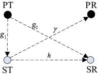
Refer to caption — Fig. 1: System model of the cognitive radio network.

One data frame of CR is divided into the sensing slot with duration $\tau$ and the transmission slot with duration $T-\tau$ . During the sensing slot, ST listens to the primary channel and obtains its accumulated energy. In the conventional schemes, spectrum sensing is performed in this slot and the decisions on the status (active/idle) of the channels are made. When transmitting, ST accesses the primary band with the optimal power in order to maximize the throughput while at the same time keeping the interference to PR.

During the sensing slot, the $j$ th received sample symbol at ST is

r_{j}=\left\{\begin{aligned} &n_{j},&H_{0},\\ &\sqrt{g_{1}}s_{j}+n_{j},&H_{1},\end{aligned}\right.

(1)

where $H_{0}$ and $H_{1}$ denote the hypothesis that PT is absent and present, respectively; $n_{j}$ is the additive noise which is assumed to follow a circularly symmetric complex Gaussian distribution with zero mean and variance $N_{0}$ , i.e., $n_{j}\backsim{\cal N}_{c}(0,N_{0})$ ; $s_{j}$ is the $j$ th symbol transmitted from PT. For the purpose of computing the achievable channel rate, the transmitted symbols $s_{j}$ from the Gaussian constellation are typically assumed [4, 5], i.e., $s_{j}\backsim{\cal N}_{c}(0,P_{p})$ , where $P_{p}$ is the symbol power. Without loss of generality, we assume that $s_{j}$ and $n_{j}$ are independent of each other.

The detection statistic $x$ using the accumulated received sample energy can be written as

x=\sum_{j=1}^{\tau f_{s}}|r_{j}|^{2},

(2)

where $f_{s}$ is the sampling frequency at ST. Then the probability density functions (pdf), conditioned on $H_{0}$ and $H_{1}$ , are given by

		$\displaystyle f(x\|H_{0})=\frac{x^{\tau f_{s}-1}e^{-\frac{x}{N_{0}}}}{\Gamma(\tau f_{s})N_{0}^{\tau f_{s}}},$		(3)
		$\displaystyle f(x\|H_{1})=\frac{x^{\tau f_{s}-1}e^{-\frac{x}{N_{0}+g_{1}P_{p}}}}{\Gamma(\tau f_{s})(N_{0}+g_{1}P_{p})^{\tau f_{s}}},$		(3)

where $\Gamma(.)$ is the gamma function defined as $\Gamma(x)=\int_{0}^{+\infty}t^{x-1}e^{-t}dt$ .

In the conventional CR, ST compares $x$ with a threshold $\rho$ , and makes decision according to $x\mathop{\gtrless}\limits_{H_{0}}^{H_{1}}\rho$ . Specifically:

•

In opportunistic spectrum access approach, ST can only access the primary band when $x<\rho$ (it means $H_{0}$ );
•

In sensing-based spectrum sharing, if $x<\rho$ , ST transmits with one higher power and otherwise with a lower power (binary power);
•

In underly approach, ST transmits with a constant power for all $x$ according to the interference constraint at PU (constant power). No sensing time slot is needed.

III Proposed Multiple-Level Power Allocation Strategy

It can be easily realized that the conventional constant or binary power of SU does not fully exploit the capability of the co-existing transmission. Motivated by this, we propose a multiple-level power allocation strategy for SU to improve the average achievable rate.

III-A Strategy of Multiple-Level Power Allocation

Define $\{\Re_{1},...,\Re_{M}\}$ as $M$ disjoint spaces of the receiving energy $x$ , and $\{P_{1},...,P_{M}\}$ as the corresponding allocated power of SU. Then the proposed power allocation strategy can be written as

\displaystyle P(x)=\sum_{i=1}^{M}P_{i}I_{x\in\Re_{i}},

(4)

where $I_{A}$ is the indicating function that $I_{A}=1$ if $A$ is true and $I_{A}=0$ otherwise. Note that, the conventional power allocation rules are special cases when $M=1$ or $2$ .

Using (4), the instantaneous rates of SU with receiving $x$ , at the absence and the presence of PU, are given by

		$\displaystyle R(x)\|_{H_{0}}=\sum_{i=1}^{M}\textup{log}_{2}\left(1+\frac{P_{i}h}{N_{0}}\right)I_{x\in\Re_{i}},$		(5)
		$\displaystyle R(x)\|_{H_{1}}=\sum_{i=1}^{M}\textup{log}_{2}\left(1+\frac{P_{i}h}{N_{0}+g_{2}P_{p}}\right)I_{x\in\Re_{i}},$		(6)

respectively. Then the average throughput of SU for the proposed multiple-level power allocation strategy using the total probability formula can be formulated as

\displaystyle R=

\displaystyle\frac{T-\tau}{T}\sum_{i=1}^{M}\left[q_{0}\textup{log}_{2}\left(1+\frac{P_{i}h}{N_{0}}\right)p_{i,0}+q_{1}\textup{log}_{2}\left(1+\frac{P_{i}h}{N_{0}+g_{2}P_{p}}\right)p_{i,1}\right],

(7)

where $q_{0}$ and $q_{1}=1-q_{0}$ are the idle and busy probabilities of the PU respectively; $p_{i,0}=\textup{Pr}(x\in\Re_{i}|H_{0})$ and $p_{i,1}=\textup{Pr}(x\in\Re_{i}|H_{1})$ , which can be directly computed from (3) and are functions of $\tau$ .

In order to keep the long-term power budget of SU, the average transmit power, denoted by $\bar{P}$ , is constrained as

\displaystyle\frac{T-\tau}{T}\sum_{i=1}^{M}P_{i}\left[q_{0}p_{i,0}+q_{1}p_{i,1}\right]\leq\bar{P}.

(8)

Moreover, to protect the QoS of PU, an interference temperature constraint should be applied too. Under (4), the interference is caused only when the PU is present. Denoting $\bar{I}$ as the maximum average allowable interference at PU, the average interference power constraint can be formulated as

\displaystyle\frac{T-\tau}{T}\sum_{i=1}^{M}\gamma q_{1}P_{i}p_{i,1}\leq\bar{I}.

(9)

Our target is to find the optimal space division $\{\Re_{i}\}$ ,¹¹ 1 Namely, we have multiple thresholds to categorize $x$ rather than only using $\rho$ in convention. the power allocation $\{P_{i}\}$ , as well as the sensing time $\tau$ in order to maximize the average achievable rate of SU under the power constraints. The optimization is then formulated as

		$\displaystyle\mathop{\textup{}}{max}\limits_{\tau,P_{i},\Re_{i}}~R~$
		$\displaystyle~~\textup{s.t}.~(\ref{eq1c32}),~(\ref{eq1c34}),~0\leq\tau\leq T,~P_{i}\geq 0,~\forall i.$		(10)

The term $\frac{T-\tau}{T}$ means that the power constraints occur in the transmission slot. Note that (10) is nonlinear and non-convex over $\tau$ . Hence, following [4, 7], we will simply use the one-dimensional search within the interval $[0,T]$ to find the optimal $\tau$ , whose complexity is generally acceptable as known from [8, 9].

III-B Finding the Solutions

The Lloyd’s algorithm is employed here to solve the problem (10), where local convergence has been proved for some cases in one-dimensional space. But in general, there is no guarantee that Lloyd¡¯s algorithm will converge to the global optimal [10]. Starting from a feasible solution as the initial value, e.g., subspaces $\{\Re_{i}\}$ satisfying $p_{i,0}=\frac{1}{M}$ , we repeat the following two steps until the convergence: Step 1) determine the power allocations $\{P_{i}\}$ given the subspaces $\{\Re_{i}\}$ ; Step 2) determine the subspaces $\{\Re_{i}\}$ given power allocations $\{P_{i}\}$ .

Subspaces Design: First, we demonstrate that the design of the optimal subspace division $\{\Re_{i}\}$ and power allocation $\{P_{i}\}$ is equivalent to a modified distortion measure design [11]. Incorporating the power constraints by the Lagrange multipliers $\lambda$ and $\mu$ , we define the following distortion measure for optimizing the rate

	$\displaystyle R(x,P_{i})=$	$\displaystyle q_{0}\textup{log}_{2}\left(1+\frac{P_{i}h}{N_{0}}\right)f(x\|H_{0})-\mu q_{1}\gamma P_{i}f(x\|H_{1})+q_{1}\textup{log}_{2}\left(1+\frac{P_{i}h}{N_{0}+g_{2}P_{p}}\right)f(x\|H_{1})$
		$\displaystyle-\lambda P_{i}\left[q_{0}f(x\|H_{0})+q_{1}f(x\|H_{1})\right].$		(11)

The optimization problem in (10) is equivalent to selecting $\{\Re_{i}\}$ and $\{P_{i}\}$ to maximize the average distortion given by

R=\frac{T-\tau}{T}\sum_{i=1}^{M}\int_{x\in\Re_{i}}R(x,P_{i})dx.

(12)

The optimal subspaces $\{\Re_{i}\}$ are then determined by the farthest neighbor rule as

\Re_{i}=\{x:~R(x,P_{i})\geq R(x,P_{k}),~\forall k\neq i\}.

(13)

The following lemma is instrumental to deriving the optimal subspaces $\{\Re_{i}\}$ .

Lemma 1: For $x_{1}<x_{2}<x_{3}$ , if $x_{1}\in\Re_{i}$ , $x_{2}\in\Re_{k}$ and $i\neq k$ , then $x_{3}\notin\Re_{i}$ must hold.

Proof:

Define the following function

\displaystyle S_{i,k}(x)=R(x,P_{i})-R(x,P_{k})=\frac{x^{\tau f_{s}-1}e^{-\frac{x}{N_{0}}}}{\Gamma(\tau f_{s})}\left[\frac{a_{i,k}}{(N_{0}+g_{2}P_{p})^{\tau f_{s}}}e^{\frac{xg_{2}P_{p}}{N_{0}(N_{0}+g_{2}P_{p})}}+\frac{b_{i,k}}{N_{0}^{\tau f_{s}}}\right],

where $a_{i,k}=q_{1}\left[\textup{log}_{2}\left(1+\frac{P_{i}h}{N_{0}+g_{2}P_{p}}\right)-\textup{log}_{2}\left(1+\frac{P_{k}h}{N_{0}+g_{2}P_{p}}\right)\right]-\lambda q_{1}(P_{i}-P_{k})-\mu q_{1}\gamma(P_{i}-P_{k}),$ $b_{i,k}=q_{0}\left[\textup{log}_{2}\left(1+\frac{P_{i}h}{N_{0}+g_{2}P_{p}}\right)-\textup{log}_{2}\left(1+\frac{P_{k}h}{N_{0}+g_{2}P_{p}}\right)\right]-\lambda q_{0}(P_{i}-P_{k}).$ From $x_{1}\in\Re_{i}$ , $x_{2}\in\Re_{k}$ and (13), we can get that $S_{i,k}(x_{1})>0$ and $S_{i,k}(x_{2})<0$ . In (13), the sign of $S_{i,k}(x)$ is decided by $\frac{a_{i,k}}{(N_{0}+g_{2}P_{p})^{\tau f_{s}}}e^{\frac{xg_{2}P_{p}}{N_{0}(N_{0}+g_{2}P_{p})}}+\frac{b_{i,k}}{N_{0}^{\tau f_{s}}}$ which is a strictly monotonic function. Thus for any $x_{3}>x_{2}$ , there are $S_{i,k}(x_{3})<0$ and $x_{3}\notin\Re_{i}$ . ∎

Assuming that the range of $x$ can be divided into more than $M$ continuous intervals, we immediately know from the drawer principle that more than 2 intervals belong to the same subspace which is contradicted with Lemma 1. Thus we can conclude that, the range of $x$ should be divided into $M$ continuous intervals. Define $M+1$ thresholds $\eta_{0},~\eta_{1},...,\eta_{M}$ with $\eta_{0}=0$ , $\eta_{M}=+\infty$ . Thus $\Re_{i}$ corresponds to one of $[\eta_{j-1},\eta_{j}),~j=[1,...,M]$ . Based on Lemma 1, we can calculate $\eta_{j}$ sequentially and assign $\{\Re_{i}\}$ in Table I. The answer of $x_{k}$ that satisfies $S_{i,k}(x_{k})=0$ is given by

\displaystyle x_{k}=\frac{N_{0}(N_{0}+g_{2}P_{p})}{g_{2}P_{p}}\cdot\textup{In}\left(\frac{-b_{i,k}(N_{0}+g_{2}P_{p})^{\tau f_{s}}}{a_{i,k}N_{0}^{\tau f_{s}}}\right).

(14)

TABLE I:

Subspaces design for $x$ given $\{P_{i}\}$
$\blacktriangleright$ Initialize the set $\Theta=\{1,...,M\}$ ; Set $i=\textup{arg}\mathop{\textup{}}{max}\limits_{j\in\Theta}R(0,P_{j})$ , $\Theta\leftarrow\Theta\backslash i$
$\blacktriangleright$ For $l=1:M-1$ , do
1) Calculate $x_{k}$ that satisfies $S_{i,k}(x_{k})=0,k\in\Theta$
2) Set $\eta_{l}=\mathop{\textup{}}{min}\limits_{k\in\Theta}x_{k}$ . Assign $\Re_{i}=[\eta_{l-1},\eta_{l})$
3) Set $i=\textup{arg}\mathop{\textup{}}{min}\limits_{k\in\Theta}x_{k}$ , $\Theta\leftarrow\Theta\backslash i$
$\blacktriangleright$ End for
$\blacktriangleright$ Set the last element in $\Theta$ as $i$ , $\Re_{i}=[\eta_{M-1},\eta_{M})$

Power Allocation: After obtaining the threshold $\eta_{i}$ , the probabilities $p_{i,j}$ in (10) can be explicitly expressed as

p_{i,j}=\int_{\eta_{i-1}}^{\eta_{i}}f(x|H_{j})dx,~i\in[1,...,M],~j=0,1.

(15)

First we write the lagrangian $L(P_{i},\lambda,\mu)$ for problem (10) under the constraints (8) and (9) as

\displaystyle L(P_{i},\lambda,\mu)=

\displaystyle R+\lambda\left(\bar{P}-\frac{T-\tau}{T}\sum_{i=1}^{M}P_{i}\left[q_{0}p_{i,0}+q_{1}p_{i,1}\right]\right)+\mu\left(\bar{I}-\frac{T-\tau}{T}\sum_{i=1}^{M}q_{1}\gamma P_{i}p_{i,1}\right),

(16)

where $\lambda,~\mu\geq 0$ are dual variables corresponding to (8) and (9). The lagrange dual optimization can be formulated as

\displaystyle\mathop{\textup{}}{min}\limits_{\lambda\geq 0,~\mu\geq 0}~~g(\lambda,\mu)\triangleq\sup_{P_{i}\geq 0}L(P_{i},\lambda,\mu).

(17)

In (10), $\frac{\partial^{2}R}{\partial^{2}P_{i}}=-\frac{T-\tau}{T}\left\{\frac{\textup{log}_{2}(e)q_{0}p_{i,0}}{(P_{i}+N_{0}/h)^{2}}+\frac{\textup{log}_{2}(e)q_{1}p_{i,1}}{(P_{0}+(N_{0}+g_{2}P_{p})/h)^{2}}\right\}<0$ , and $\frac{\partial^{2}R}{\partial P_{i}\partial P_{j}}=0,i\neq j$ . Since the constraints are linear functions, problem (10) is concave over $P_{i}$ . Thus the optimal value $P_{i}$ of problem (17) is equal to that of (10), and we can solve (17) instead of (10). From (17), we have to obtain the supremum of $L(P_{i},\lambda,\mu)$ . Taking the derivative of $L(P_{i},\lambda,\mu)$ with respect to $P_{i}$ leads to

\displaystyle\frac{\partial L(P_{i},\lambda,\mu)}{\partial P_{i}}=

\displaystyle\frac{T-\tau}{T}\left\{\frac{\textup{log}_{2}(e)q_{0}p_{i,0}}{P_{i}+N_{0}/h}+\frac{\textup{log}_{2}(e)q_{1}p_{i,1}}{P_{i}+(N_{0}+g_{2}P_{p})/h}-\lambda\left[q_{0}p_{i,0}+q_{1}p_{i,1}\right]-\mu q_{1}\gamma p_{i,1}\right\}.

(18)

By setting the above equation to 0 and applying the constraint $P_{i}\geq 0$ , the optimal power allocation $P_{i}$ for given Lagrange multipliers $\lambda$ and $\mu$ is computed as

\displaystyle P_{i}=\left[\frac{A_{i}+\sqrt{\triangle_{i}}}{2}\right]^{+},

(19)

where $[x]^{+}$ denotes $\textup{max}(0,x)$ , and

	$\displaystyle A_{i}=$	$\displaystyle\frac{\textup{log}_{2}(e)\left[q_{0}p_{i,0}+q_{1}p_{i,1}\right]}{\lambda\left[q_{0}p_{i,0}+q_{1}p_{i,1}\right]+\mu q_{1}\gamma p_{i,1}}-\frac{2N_{0}+g_{2}P_{p}}{h},$		(20)
	$\displaystyle\triangle_{i}=$	$\displaystyle A_{i}^{2}+\frac{4}{h}\left\{\frac{\textup{log}_{2}(e)\left[q_{0}p_{i,0}(N_{0}+g_{2}P_{p})+q_{1}p_{i,1}N_{0}\right]}{\lambda\left[q_{0}p_{i,0}+q_{1}p_{i,1}\right]+\mu q_{1}\gamma p_{i,1}}-\frac{N_{0}(N_{0}+g_{2}P_{p})}{h}\right\}.$		(21)

Proposition 1: The power allocation functions $P_{i}$ are non-increasing over $i$ .

Proof:

First, from (3), we have

\frac{f(x|H_{1})}{f(x|H_{0})}=e^{\frac{xg_{1}P_{p}}{N_{0}(N_{0}+g_{1}P_{p})}}\left(\frac{N_{0}}{N_{0}+g_{1}P_{p}}\right)^{\tau f_{s}},

(22)

and obviously it is an increasing function over $x$ . Through some simple manipulations, the monotonicity of $A_{i}$ is equivalent to the monotonicity of the following term

C_{i}=\frac{1+\frac{q_{1}}{q_{0}}\frac{p(i,1)}{p(i,0)}}{1+(1+\mu\gamma/\lambda)\frac{q_{1}}{q_{0}}\frac{p(i,1)}{p(i,0)}}.

(23)

From (22), we can get that

\frac{p(i,1)}{p(i,0)}>\frac{p(i+1,1)}{p(i+1,0)},~\forall i.

(24)

Jointly from (23) and (24), we know that $A_{i}$ is a decreasing function over $i$ . Similarly, we can also prove that $\triangle_{i}$ is a decreasing function over $i$ . Thus from (19), we can conclude that, $P_{i}$ is a non-increasing function with respect to $i$ . ∎

Remark: Proposition 1 shows that, at smaller $x$ the probability of PU being busy is smaller, so SU can use higher transmit power to better exploit the primary band; On the other hand, at the larger $x$ , lower transmit power should be used to prevent harmful interference to PU. Thus the proposed multiple-level power allocation strategy can also be defined on the the probability of the PU being busy.

Subgradient-based methods are used here to find the optimal Lagrange multipliers $\lambda$ and $\mu$ , e.g., the ellipsoid method and the Newton’s method [12]. The subgradient of $g(\lambda,\mu)$ is $[C,D]^{T}$ , where

		$\displaystyle C=\bar{P}-\frac{T-\tau}{T}\sum_{i=1}^{M}\bar{P}_{i}\left[q_{0}p_{i,0}+q_{1}p_{i,1}\right],$
		$\displaystyle D=\bar{I}-\frac{T-\tau}{T}\sum_{i=1}^{M}q_{1}\gamma\bar{P}_{i}p_{i,1},$		(25)

while $\bar{P}_{i}$ is the optimal power allocation for fixed $\lambda$ and $\mu$ [13]. Finally, we summarize the algorithm that computes the sensing time and multiple-level power allocations in Tab.II.

Remark 2: All computations are performed offline and the resulting power control rule is stored in a look-up table for real-time implementation. Thus the computational complexity is not significant.

TABLE II:

Sensing time and multiple-level power allocations
$\blacktriangleright$ For each $\tau$ in $[0,T]$ , do
1) Initialize $\lambda$ , $\mu$ , $\eta_{i}$ satisfying $p_{i,0}=\frac{1}{M}$
2) Repeat until $\{\Re_{i}\}$ converge:
- Get $\{P_{i}\}$ using (19); Update $\lambda$ and $\mu$ using the
subgradient-based method; Until $\lambda$ and $\mu$ converge
- Update $\{\Re_{i}\}$ using Table I
$\blacktriangleright$ End for
$\blacktriangleright$ Optimal parameters: $\tau^{}=\mathop{\textup{}}{argmax}\limits_{\tau}R(\tau,P_{i},\Re_{i})$ , $\left(P_{i}^{},\Re_{i}^{}\right)=\left(P_{i},\Re_{i}\right)\|_{\tau=\tau^{}}$

IV Simulation results

In this section, simulations are performed to evaluate the proposed multiple-level power allocation strategy in a CR system where the system parameters similar to the references [4, 5, 7] are used. The frame duration is taken as $T=100$ ms and the sampling frequency $f_{s}=1$ MHz. The target detection probability is set to $0.9$ in the opportunistic spectrum access scheme. We set $g_{1}=N_{0}=0$ dB, $q_{0}=0.7$ , $\bar{I}=P_{p}=0.5$ , $\bar{P}=10$ dB, $\gamma=h=g_{2}=0$ dB, and unless otherwise mentioned.

Fig. 2 compares the power allocations under the conventional strategies as well as the proposed one. The figure shows that $P_{i}$ for the proposed strategy is a non-increasing function of the received signal energy. When $x$ is small, the proposed strategy allocates more power than the conventional ones, while when $x$ is large, it allocates less power, thus the average transmit powers are the same for all the strategies.

Fig. 3 shows the average secondary achievable rate. In the low $\bar{P}$ region, the proposed strategy and the conventional ones have the same rates. However, when $\bar{P}$ is high, the proposed strategy achieves much higher rates. The rates of all strategies flatten out when $\bar{P}$ is sufficiently large since the rate is decided by $\bar{I}$ under this condition. When $M$ increases, the rate of the proposed strategy becomes larger, but the gain does not improve much when $M$ is large. As $M$ becomes extremely large, say $M=1000$ in the figure, the rate approaches an upper limit. In practice, we can choose the right $M$ to tradeoff the system complexity and performance, and in this example $M=4$ serves as a good choice.

V Conclusions

In this paper, we propose a new multiple-level power allocation strategy for SU in a CR system. The receiving signal energy from PU is divided into different categories and SU transmits with different power for each category. It is known that the conventional CR strategies are special cases of the proposed one. The power levels at SU are obtained by maximizing the average achievable rate under the constraints of the average transmit power at SU and the average interference power at PU. Compared with the conventional power allocation strategies, the proposed scheme offers significant rate improvement for SU.

References

[1] Q. Wu, G. Ding, J. Wang, Y. D. Yao, “Spatial-temporal opportunity detection for spectrum-heterogeneous cognitive radio networks: two-dimensional sensing,” IEEE Trans. Wirel. Commun., vol. 12, no. 2, pp. 516-526, Feb. 2013.
[2] S. Stotas and A. Nallanathan, “On the throughput and spectrum sensing enhancement of opportunistic spectrum access cognitive radio networks,” IEEE Trans. Wireless Commun., vol. 11, no. 1, pp. 97-107, Jan. 2012.
[3] X. W. Gong, S. A. Vorobyov, and C. Tellambura, “Optimal bandwidth and power allocation for sum ergodic capacity under fading channels in cognitive radio networks,” IEEE Trans. Signal Process., vol. 59, no. 4, pp. 1814-1826, Apr. 2011.
[4] R. F. Fan, J. Hai, Q. Guo, and Z. Zhang, “Joint optimal cooperative sensing and resource allocation in multichannel cognitive radio networks,” IEEE Trans. Veh. Technol., vol. 60, no. 2, pp. 722-729, Feb. 2011.
[5] X. Kang, Y. C. Liang, H. K. Garg, L. Zhang, “Sensing-based spectrum sharing in cognitive radio networks,” IEEE Trans. Veh. Technol., vol. 58, no. 8, pp. 4649-4654, Oct. 2009.
[6] Z. Chen, F. Gao, X. D. Zhang, J. Li, M. Lei, “Sensing and power allocation for cognitive radio with multiple primary transmit powers,” IEEE Wirel. Commun. Lett., DOI: 10.1109/WCL.2013.030613.130014, pp. 1-4, 2013.
[7] Y. Y. Pei, Y. C. Liang, Y. C. Teh, and K. H. Li, “How much time is needed for wideband spectrum sensing?” IEEE Trans. Wireless Commun., vol. 8, no. 11, pp. 5466-5471, Nov. 2009.
[8] R. O. Schmidt, “A Signal Subspace Approach to Multiple Source Location and Spectral Estimation,” Ph.D. dissertation, Stanford Univ., Stanford, CA, May 1981.
[9] H. Liu and U. Tureli, “A high-efficiency carrier estimator for OFDM communications,” IEEE Commun. Lett., vol. 2, no. 4, pp. 104-106, Apr. 1998.
[10] S. P. Lloyd, “Least-square quantization in PCM,” IEEE Trans. Inform. Theory, vol. IT-28, pp. 129-137, Mar. 1982.
[11] V. Lau, Y. Liu, T. -A. Chen, “On the design of MIMO blockfading hannels with feedback-link capacity constraint,” IEEE Trans. Commun., vol. 52, no. 1, pp. 62-70, Jan. 2004.
[12] S. Boyd and L. Vandenberghe, Convex Optimization, Cambridge, UK: Cambridge University Press, 2005.
[13] D. P. Bertsekas. Convex Analysis and Optimization. Athena Scientific, 2003.