Electrons turn into anyons under an elastic membrane
Abstract
We show that electrons acquire anyonic statistics if a two-dimensional electron gas is placed in proximity to a charged magnetic membrane. In this two-layered system, electrons become anyons through electromagnetic field mediated interactions with a membrane phonon. The statistical parameter is irrational and depends on the membrane tension and on the electric charge and magnetic dipolar densities on the membrane. We propose a measurement that yields the value of the statistical parameter.
I introduction
Anyons are particles whose wavefunctions acquire a nontrivial phase upon exchange of coordinates, i.e., a phase factor other than that for bosons () or fermions () [1, 2]. Anyons are possible in two spatial dimensions (2D), where the braiding of the worldlines of the particles is non-trivial. Quasiparticle excitations that obey Abelian anyonic exchange statistics, as well as non-Abelian extensions, are theoretically predicted to exist in fractional quantum Hall (FQH) states [5, 6]. Much effort, in the form of theoretical proposals [7, 8] and experimental attempts [9, 10, 11, 12], has been devoted to the detection of both Abelian and non-Abelian anyons in FQH liquids.
In the FQH effect, the elementary quasiparticle excitations carry both rational fractional charges and rational statistics (the phases are rational multiples of ) [3, 4, 5, 6]. This “rationality” is rooted in the connection of the FQH effect and Chern-Simons theory [13, 14, 15, 16, 17], from which it also follows that the many-body ground state is degenerate on closed surfaces, with the degeneracy depending on the surface genus [18, 19].
Anyons, however, need not be always rational like in the FQH effect. The statistical angles can in principle take irrational values [2], once the physical origin of the anyonic statistics is divorced from Chern-Simons theory. One example where the statistical angle can vary continuously is when the quasiparticles are associated to vortices in a complex mass order parameter (a Higgs field) for 2D Dirac electrons [20, 21]. In these examples both the quasiparticle charge and statistics can vary continuously, but then the vortices are logarithmically confined. The vortices can be deconfined with the addition of an axial gauge field [22], but when they are, the charge and statistics become rational again [20, 21].
The goal of this work is to point out that, given a recently suggested alternative framework for realizing anyonic statistics [23], it is possible to turn ordinary electrons into anyons. This mutation, we show, occurs when a 2D electron gas (2DEG) is placed under an elastic electric and magnetic membrane. In this two-layered system, the anyons reside on the 2DEG layer. The essence of the mechanism is that height fluctuations of the membrane generate fluctuations in the gauge potential seen by the electrons in the 2DEG below, while the charge density of the electrons can affect the height fluctuations of membrane above. Hence, the membrane fluctuations act as a middle man, allowing the electron charge to directly source the magnetic field. This is sufficient to turn an electron into an anyon.
Under the elastic membrane, the electric charge of the particle is rational (in fact, integer), but the statistical angle is not forced to take rational values. Instead, it depends continuously on the elastic membrane tension, , as well as on the electric charge and magnetic dipole densities on the membrane. The statistical angle is , where
| (1) |
We present the mechanism behind the statistical transmutation of electrons into anyons under the electric and magnetic membrane, and argue that there is an experimentally accessible regime where the effect could be probed.
The basic observation underlying the change in electron statistics is the fact that in 2+1 dimensions a gauge field has the same degrees of freedom as a scalar. Thus, the anyonic phenomena can be obtained via the replacement of the spatial components of a statistical gauge field, , by a scalar field: . In terms of the scalar, the statistical magnetic field . We conclude that anyons will result if we can arrange that the electron field, , serves as a source for ,
| (2) |
while at the same time enjoying a coupling to it through a “covariant derivative” which mimics the effects of a gauge field :
| (3) |
In this framework, the statistical parameter is given in terms of the couplings and as , and can be any real number.
An action which leads to (2) (at sufficiently large distances) and (3) is
| (4) | |||||
The first line describes the height fluctuations of a membrane under tension . The term is the extrinsic curvature contribution to the membrane bending energy, and is the surface mass density. Our task in what follows will be to induce the couplings on the second and third line above between an electron and the membrane phonon. We will see that this is possible through the electromagnetic fields due to electric charges and magnetically aligned dipoles on the elastic membrane.
II Potentials under the membrane
Consider a magnetic membrane, with an areal density of magnetic dipolar moments that are aligned along the normal to the membrane. The orientation of the dipoles can be fixed by a perpendicular external magnetic field. We note that because of the external field, one can equally use a paramagnetic or ferromagnetic system. In addition, let the membrane posses a charge density, . Also consider a metallic sheet, with some electronic density a distance away from the membrane. For simplicity we assume that the separation is much smaller than the length of the membrane. The configuration is depicted in Fig. 1.
We assume the following Hamiltonian for electrons on the metallic sheet:
| (5) |
Here is the electric potential, and is the magnetic vector potential.
Our first task is to calculate the vector potential on the metallic sheet induced by the height fluctuations of the membrane. In this calculation we assume that the surface of the magnetic membrane fluctuates while the dipolar moments are fixed in the direction. This assumption is reasonable for two reasons. The first is that corrections due to the tilting of the dipoles is of higher order in gradients of . The second is that the tilting of the dipoles is gapped by the external field that aligns the spins along the direction.
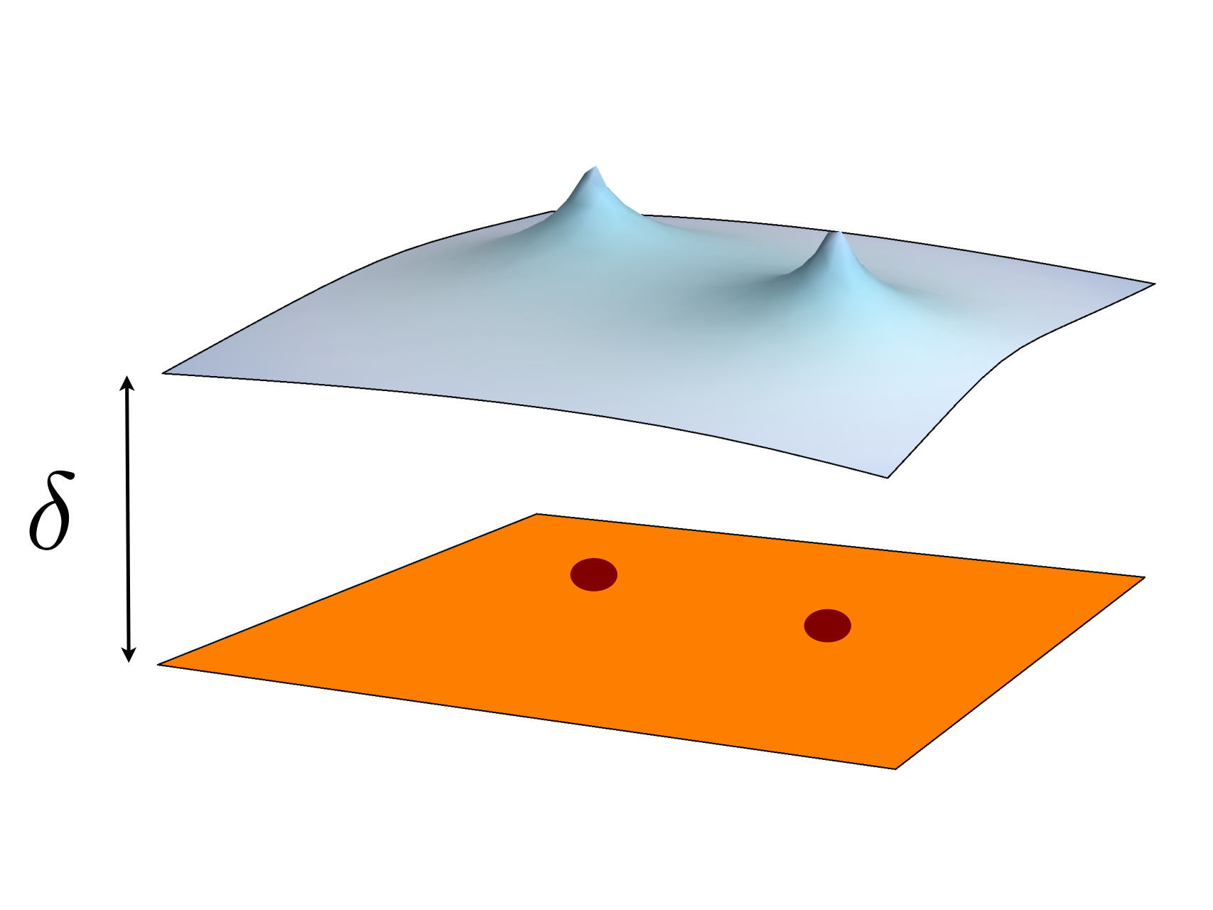
We assign the surface coordinate to the membrane and to the metallic sheet. The vector potential on the metallic sheet is calculated from
| (6) |
where is the height fluctuation of the membrane around its average position . (Notice that if the membrane is placed above the metallic sheet, and when the membrane is below.) We also introduced
| (7) |
which is related to by considering the tilting of the normal direction. In the absence of height fluctuations, the magnetic membrane induces a constant magnetic field on the metallic sheet. Therefore we can decompose the vector potential as
| (8) |
The contribution leads to a uniform background field, which can be added to the externally applied field. The contribution is due to the height fluctuations of the membrane. We assume that these fluctuations are smooth on the scale of . As we show in the Appendix, the vector potential fluctuation is
| (9) |
Notice that to leading order the vector potential is independent of the magnitude of , but it depends on its sign, i.e., on whether the membrane placed above or below the electronic plane.
A very similar calculation leads to the dependence of the electric potential on the membrane fluctuation:
| (10) |
Here, as above, we have ignored the uniform background electric field in the direction.
Comparing (4) with (5) we can read off the couplings of the membrane phonons with the electrons of the metallic layer:
| (11) |
Thus, in terms of the membrane parameters, the statistical angle is given by the expression presented in Eq. (1). We note that can be any real number, and can be varied experimentally. Next, we discuss an experimental setup to measure the statistical parameter .
III Proposed experimental setup
Consider the geometry depicted in Fig. 2, where a metallic ring and a central metallic island are defined on the 2DEG plane. The island could be charged by a back gate. The proposed measurement consists of studying the oscillations of the conductance through the ring as function of the charge in the island. These oscillations arise because the charge in the island vertically displaces the membrane, which in turn generates a magnetic flux for the electrons in the ring. For the electrons confined to the plane of the 2DEG, unaware of the membrane in the third dimension, the accumulated quantum mechanical phase is due to anyonic statistics.

Let us compute the Aharonov-Bohm (AB) phase accumulated by the electrons in the ring when one charges up the island with charge . The deformation of the membrane follows from the equations of motion for the displacement :
| (12) |
where and are, respectively, the electron number and current densities on the 2DEG plane. Let us focus on the case where the charge in the island is static (). Because the island is metallic, the charge will concentrate at its edges. To compute the magnetic flux through a region encircling the island, due to the charge within, we use that (9) implies that , which gives
| (13) |
This result means that flux is affixed to the charge . The particles are a meld of charge and flux, and it is this composite nature that gives rise to the anyonic statistics.
The flux in (13) is in addition to any other flux due to externally applied magnetic fields. The conductance through the ring, , oscillates as function of with period ( in natural units where ). Now, the charge in the island is quantized, , . Thus can only change in steps as the charge is varied by changing the back gate (, where is the capacitance of the island). Every time extra electrons are added to the island, the pattern of AB oscillations in the conductance is shifted by a phase . So measurements for different values of back gate voltages should yield a family of phase shifted patterns of AB oscillations in the conductance as function of the externally applied flux . The shift in the patterns is .
The statistical parameter of the anyons can then be determined from measurements of and :
| (14) |
A comment is in order. The coupling of the electrons in the 2DEG with the phonon mode in the membrane leads to an effective logarithmic potential between the electrons. A possible worry is then that a dynamical phase accumulates as the electrons go around the ring. Such a phase would depend on the detailed shape of the ring. The reason why this additional dynamical phase is not present is that the ring is metallic, and therefore charges can redistribute so as to bring the total potential (the sum of effective plus electric potentials) to a constant value throughout the ring. As long as the width of the ring is smaller than the distance to the membrane, these redistributed charges will not affect the membrane displacement above the ring. Consequently, the electromagnetic field generated by the membrane will not be affected, which means that the AB-phase will not be disturbed.
III.1 Possible realizations
Let us discuss possible examples of such two-layered magnetic/electronic system. There are many possibilities for the 2DEG, for example Si or a semiconductor GaAs/AlGaAs heterostructure. The ability to gate the electron gas, so as to define an Aharonov-Bohm ring and an island, is important. Alternatively, one could just deposit thin metallic (say gold) layers on a substrate, and write directly the wire and island with metal. Essential is the ability to back gate the island, to control the electron density in it.
As for the possible realization of the electric and magnetic membrane, perhaps the ideal candidate would be a suspended graphene sheet that is doped with magnetic ions. The polarized membrane would result from an externally applied field. By electrically biasing the membrane, one could charge it too. It would thus be possible to control both the charge and magnetic dipole densities and .
Let us first estimate the size of the various effects we have discussed in this particular realization. We will only provide an order of magnitude estimate. Magnetic impurities spaced about away, with each impurity having a magnetic moment of order , yields a magnetic density of order . As for the membrane tension and surface charge density, it is more suiting to work with the membrane displacements directly. We shall work with the constraint that the maximum displacement does not exceed the order of . (The distance can be taken to be of order of safely if the membrane is poped upwards.)
If the membrane is clamped (Dirichlet boundary conditions) at a radius from the center of the island (see Fig. 2), then the displacement due to a charge in the island of radius is
| (15) |
We shall consider and . The AB ring width must fit within this gap, so a width of is reasonable.
One can express the statistical phase in terms of the maximum displacement of the membrane, at the edge of the island:
| (16) | |||||
The statistical phase an electron in the ring feels as a result of all the electrons in the island is
| (17) | |||||
We remark that using ions with magnetic moment larger that one Bohr magneton and increasing the density of magnetic dopants could raise this number by one or two orders of magnitude. Furthermore, a larger maximum displacement and larger radius (keeping constant the difference ) can increase the effect by perhaps another order of magnitude.
Finally, the value of will ultimately depend on the tension and electric charge density. Because the bending rigidity in graphene is , there is a characteristic scale which needs to be kept smaller than the dimensions in the proposed experimental set up (say ). We can express the membrane displacement as . Parameterizing the charge density as , with one would have a charge of about per atom in the membrane. We thus find that . Therefore the phase picked by the electrons around the AB ring is sizable even for very few electrons in the island.
IV Conclusions
In this paper we have shown that it is possible to turn electrons into anyons if they are placed under an elastic membrane that is both charged and magnetized. We have also proposed an experimental set up to detect the anyonic statistics, and estimated the size of the measurable phases for a possible concrete experimental realization using patterned metallic rings and islands under a suspended graphene sheet, which could be both charged and doped with magnetic impurities.
Finally, let us point out that there is nothing intrinsic to our general “membrane” mechanism which necessitates that the “electronyons” feel an induced logarithmic potential. Indeed, had we not charged the membrane at all, the electrons would still become anyons due to their Zeeman coupling to the magnetic field (albeit for distances less than , which could be made large by not tensioning the membrane). However, there would not be a logarithmic potential, as the induced coupling would be of the form . The resulting statistical parameter would be too small in this case.
One could imagine yet a different setup: instead of one membrane, there are three membranes on top of each other, with charge densities , , and , for the top, middle, and bottom membrane respectively. As long as the membranes are very close to one other, and can be made to move together, there will be an effective quadrpole charge density. This will result in a coupling of the form , which again does not induce an effective force between electrons. In this scenario, ignoring the Coulomb force between electrons, the theory will be precisely that of [23] at distances less than .
Appendix A The electric and vector potentials due to membrane fluctuations
In this Appendix we present the potentials due to the membrane phonon. We will present the vector potential calculation in detail. The electric potential is found in a very similar manner. We assign the coordinate to the membrane and to the fixed plane. We are interested in the contribution from . The vector potential on the fixed plane is calculated from:
| (18) | |||||
The -dependence of the vector potential can be extracted by linearizing in , in the regime that the membrane does not touch the 2DEG, when :
| (19) |
We are interested in small fluctuations of the field and in momenta . Consequently,
| (20) |
Here is the Fourier transform of , and we have included the leading correction in . It is interesting to note that corrections are non-local, furthermore we see that appears with factors of , therefore the corrections decouple in the long wavelength limit. An analogous formula holds for the electric potential, , with replaced by (and with the derivative absent).
Acknowledgements.
We thank Maissam Barkeshli, Alex Kitt, and Yiming Xu for useful discussions. This work was supported in part by DOE grant DEFG02-01ER-40676 and NSF CAREER grant PHY-0645456 (SRB and EK) and DOE Grant DEFG02-06ER46316 (CC).References
- [1] J. M. Leinaas and J. Myrheim, Nuovo Cimento 37B, 1 (1977).
- [2] F. Wilczek, Phys. Rev. Lett. 49, 957 (1982).
- [3] R. B. Laughlin, Phys. Rev. Lett. 50, 1395 (1983).
- [4] F. D. M. Haldane, Phys. Rev. Lett. 51, 605 (1983)
- [5] B. I. Halperin, Phys. Rev. Lett. 52, 1583 (1984).
- [6] D. Arovas, J. R. Schrieffer, and F. Wilczek, Phys. Rev. Lett. 53, 722 (1984).
- [7] C. de C Chamon, D. E. Freed, S. A. Kivelson, S. L. Sondhi, and X.-G. Wen, Phys. Rev. B 55, 2331 (1997).
- [8] E. Fradkin, C. Nayak, A. Tsvelik, and F. Wilczek, Nucl. Phys. B 516, 704 (1998).
- [9] F. E. Camino, W. Zhou, and V. J. Goldman, Phys. Rev. B 72, 075342 (2005).
- [10] F. E. Camino, W. Zhou, and V. J. Goldman, cond-mat/0510764
- [11] R. L. Willett, C. Nayak, K. Shtengel, L. N. Pfeiffer, K. W. West, arXiv:1301.2639
- [12] Sanghun An, P. Jiang, H. Choi, W. Kang, S. H. Simon, L. N. Pfeiffer, K. W. West, K. W. Baldwin, arXiv:1112.3400
- [13] N. Read, Phys. Rev. Lett. 65, 1502 (1990).
- [14] B. Blok and X. G. Wen, Phys. Rev. B 42, 8133 (1990); ibid. Phys. Rev. B 43, 8337 (1991).
- [15] J. Fröhlich and A. Zee, 1991, Nucl. Phys. B 364, 517 (1991).
- [16] X. G. Wen and A. Zee, Phys. Rev. B 46, 2290 (1992)
- [17] J. Fröhlich and E. Thiran, J. Stat. Phys. 76, 209 (1994).
- [18] X. G. Wen, Phys. Rev. B 40, 7387 (1989).
- [19] X.-G. Wen and Q. Niu, Phys. Rev. B 41, 9377 (1990).
- [20] C. Chamon, C.-Y. Hou, R. Jackiw, C. Mudry, S.-Y. Pi, and A. P. Schnyder, Phys. Rev. Lett. 100, 110405 (2008).
- [21] S. Ryu, C. Mudry, C.-Y. Hou, and C. Chamon, Phys. Rev. B 80, 205319 (2009).
- [22] R. Jackiw and S.-Y. Pi, Phys. Rev. Lett. 98, 266402 (2007).
- [23] A. Liam Fitzpatrick, Shamit Kachru, Jared Kaplan, Emanuel Katz, and Jay G. Wacker, arXiv:1205.6816.