Discrepancy Bounds for Deterministic Acceptance-Rejection Samplers??
Abstract
We consider an acceptance-rejection sampler based on a deterministic driver sequence. The deterministic sequence is chosen such that the discrepancy between the empirical target distribution and the target distribution is small. We use quasi-Monte Carlo (QMC) point sets for this purpose. The empirical evidence shows convergence rates beyond the crude Monte Carlo rate of . We prove that the discrepancy of samples generated by the QMC acceptance-rejection sampler is bounded from above by . A lower bound shows that for any given driver sequence, there always exists a target density such that the star discrepancy is at most . For a general density, whose domain is the real state space , the inverse Rosenblatt transformation can be used to convert samples from the dimensional cube to . We show that this transformation is measure preserving. This way, under certain conditions, we obtain the same convergence rate for a general target density defined in . Moreover, we also consider a deterministic reduced acceptance-rejection algorithm recently introduced by Barekat and Caflisch [F. Barekat and R.Caflisch. Simulation with Fluctuation and Singular Rates. ArXiv:1310.4555[math.NA], 2013.]
keywords
[class=MSC] Primary 62F15 ; secondary 11K45keywords
Acceptance-Rejection Sampler , Star Discrepancy , -netsand
School of Mathematics and Statistics
The University of New South Wales, Sydney, Australia
??
1 Introduction
The Monte Carlo (MC) method is one of the widely used numerical methods for simulating probability distributions. However, sometimes it is not possible to sample from a given target distribution. Markov chain Monte Carlo (MCMC) methods have been developed to address this problem. Instead of sampling independent points directly, MCMC samples from a Markov chain whose limiting distribution is the target distribution. MCMC has widened the applications of MC in many different fields [5, 22]. Another deficiency of MC algorithms is its slow convergence rate. Quasi-Monte Carlo (QMC) algorithms on the other hand perform better in improving the convergence rate of Monte Carlo which partially depends on generating samples with small discrepancy. For a survey of QMC we refer to [10, 11]. Putting the QMC idea into MCMC is a good way to improve the convergence rate and widen practical applications. Recently many results in this direction have been achieved [6, 7, 39, 40]. With this paper we add another result in this direction by using a deterministic driver sequence in an acceptance-rejection algorithm. We prove discrepancy bounds of order , where the dimension of the state space is and is the number of samples. The discrepancy here is a generalization of the concept of the Kolmogorov-Smirnov test between the empirical distribution of the samples and the target distribution to higher dimension. A more detailed description of our results will be provided below.
1.1 Previous work on MCMC and QMC
In the following we describe some previous research on QMC and MC. L’Ecuyer studied the convergence behavior of randomized quasi-Monte Carlo for discrete-time Markov chains in [21], known as array-RQMC. The general idea is to obtain a better approximation of the target distribution than with the plain Monte Carlo method by using randomized QMC. In a different direction, Tribble [39] and Tribble and Owen [40] established a condition under which low discrepancy sequences can be used for consistent MCMC estimation for finite state spaces. It has been shown that replacing an IID sequence by a completely uniformly distributed sequence also implies a consistent estimation in finite state spaces. A construction of weakly completely uniformly distributed sequences is also proposed in [40]. As a sequel to the work of Tribble, Chen in his thesis [6] and Chen, Dick and Owen [7] demonstrated that Markov chain quasi-Monte Carlo (MCQMC) algorithms using a completely uniformly distributed sequence as driver sequence gives a consistent result under certain assumptions on the update function and Markov chain. Further, Chen [6] also showed that MCQMC can achieve a convergence rate of for any under certain conditions, but he only showed the existence of a driver sequence.
In our recent work [12], done with Rudolf, we prove upper bounds on the discrepancy under the assumptions that the Markov chain is uniformly ergodic and the driver sequence is deterministic rather than independent uniformly distributed random variables. In particular, we show the existence of driver sequences for which the discrepancy of the Markov chain from the target distribution with respect to certain test sets converges with (almost) the usual Monte Carlo rate of . A drawback of this result is that we are currently not able to give an explicit construction of a driver sequence for which our discrepancy bounds hold for uniformly ergodic Markov chains. Garber and Choppin in [14] adapted low discrepancy point sets instead of random numbers in sequential Monte Carlo (SMC). They proposed a new algorithm named sequential quasi-Monte Carlo (SQMC). They constructed consistency and stochastic bounds based on randomized QMC point set for this algorithm. It is an open problem to obtain deterministic bounds for SQMC. More literature review about applying QMC to MCMC problems can be found in [7, Section 1].
1.2 Acceptance-rejection algorithms
We now give a description of the algorithms in this paper. Let be our target density function, where and . We consider the cases where or . Assume that it is not possible to sample directly from the target distribution. One possible solution to obtain samples from is to choose a proposal density from which we can sample and then use an acceptance-rejection algorithm. Assume there exists a constant such that for all . The following algorithm can be used to obtain samples with distribution .
Algorithm 1.
(Random acceptance-rejection (RAR) algorithm). Given a target density and a proposal density . Assume that there exists a constant such that for all in the domain . We introduce another random variable having uniform distribution in the unit interval, i.e. . Then the acceptance-rejection algorithm is given by
- 1.
Draw and .
- 2.
Accept as a sample of if , otherwise go back to step 1.
See also [4, 9, 19] for a discussion of related algorithms. For a discussion on how to select proposal densities see for instance [4] and the references therein. The acceptance-rejection sampler works to sample from an unknown density based on a proposal density.
Acceptance-rejection sampling and importance sampling [34, Section 3] are quite similar ideas. Both of them distort a sample from a distribution in order to sample from another one. However, there is a difference in the selection of the constant for in the domain . The acceptance-rejection method does not work when , while importance sampling is still available [33]. In this paper, we only use the acceptance-rejection sampler to get samples of a given target density, since we are interested in obtaining discrepancy bounds for MCQMC. More information on general strategies for generating nonuniform random variables can be found in the monographs [9, 19].

The acceptance-rejection algorithm with deterministic driver sequence is one special class of MCQMC. From the superior distribution properties in terms of the discrepancy of the Sobol sequence [37] one could expect an improvement in the discrepancy of the samples obtained from the acceptance-rejection algorithm based on the Sobol sequence. In one dimension the discrepancy we study is the Kolmogorov-Smirnov test between the target distribution and the empirical distribution of the sample points. For a given point set in the -dimensional unit cube, the star discrepancy measures the difference between the proportion of points in a subinterval of and the Lebesgue measure of this subinterval. We defer the precise definition of discrepancy to Section 3.
In this paper, we replace the IID initial samples with an explicit construction of the driver sequence by using -nets [11, 27] (obtained from the Sobol sequence). Figure 1 shows a comparison between different driver sequences: deterministic points (Sobol points) and pseudo random uniform points (they both have points). The acceptance-rejection sampler works by only accepting those points under the target density curve. The difference of driver sequences will affect the samples we obtain by the acceptance-rejection algorithm, hence the distribution properties of the points which were accepted will be influenced. The right two figures in Fig.1 show the histograms of the points which we accepted in both cases. Note that the deterministic samples better estimate the density function. Our interest in this paper is in entirely deterministic methods. However, one could also use randomized quasi-Monte Carlo point sets [30, 31, 32] and study a randomized setting.
1.3 Previous work on deterministic acceptance-rejection algorithm
The deterministic acceptance-rejection algorithm has also been discussed by Moskowitz and Caflisch [24] and Wang [41, 42]. Therein a smoothing technique was introduced to improve the numerical performance of the acceptance-rejection algorithm. Wang [42] gave a heuristic argument to indicate a convergence rate of order . This argument assumes that the points in elementary intervals are uniformly distributed. Thus this reasoning is not fully deterministic. Our lower bound on discrepancy (Theorem 2) indicates that this reasoning does not apply in our case. The numerical experiments in [42] also indicate an improvement using a well chosen deterministic driver sequence (in this case the so-called Halton sequence [17]) compared to a random driver sequence. Recently, Nguyen and Ökten in [25] presented a consistency result of an acceptance-rejection algorithm for low-discrepancy sequences. This algorithm yielded good numerical performances on standard deviation and efficiency. However, proving an explicit convergence rate of the discrepancy for this algorithm is still an open problem. See also [23, 25] for numerical experiments using quasi-Monte Carlo point sets for the related problem of integrating indicator functions.
It is worth noticing that all results given in previous work are empirical evidence and the discrepancy of samples is not directly investigated. Our work focuses on discrepancy properties of points produced by totally deterministic acceptance-rejection methods. We also prove discrepancy bounds on deterministic acceptance-rejection algorithms, including an upper bound and a lower bound. The combination with the reduced acceptance-rejection sampler provides further evidence of the good performance of the deterministic method. Our algorithm here may also be combined with similar algorithms like the acceptance-complement method, see for instance [9, Section II.5].
Before presenting the theoretical background, we briefly describe deterministic algorithms and some numerical results which show a convergence rate comparison using Monte Carlo and quasi-Monte Carlo methods.
2 Our results
2.1 Construction of driver sequence
In this paper, we use low discrepancy point sets given by -sequences (see Definition 3 and Definition 4 below) in base as driver sequences. The first points of a -sequence are a so called -net in base . Explicit constructions of -sequences in base have been found by Sobol [37], in prime base by Faure [13] and in prime-power base by Niederreiter [26]. In all these constructions depends only on but not on . In practice, since digital nets (based on Sobol points) are included in the statistics toolbox of Matlab, this method is very easy to implement. People seeking more discussion of construction methods can also consult [11, Chapters 4&8].
In the following we describe the algorithm and present some numerical results. Since in general it is computationally too expensive to compute the supremum in the definition of the star-discrepancy exactly, we use a so-called -cover to estimate this supremum. An introduction to -covers is provided in the appendix. In the numerical discussion, the driver sequence is generated by a -net in base . Specifically, we always use a Sobol sequence [37] to generate -nets for our experiments.
2.2 Deterministic algorithm for target densities defined on
We consider now the case where the target density is defined on . The following algorithm is a deterministic version of Algorithm 1. For the proofs later, we need the technical assumption that the target density is pseudo-convex. The definition of pseudo-convexity is discussed in Section 3.
Algorithm 2.
(Deterministic acceptance-rejection (DAR) algorithm in ). Let the target density , where , be pseudo-convex. Assume that there exists a constant such that for all . Let . Suppose we aim to obtain approximately samples from .
- i)
Let , where is the smallest integer satisfying this inequality. Generate a -net in base .
- ii)
Use the acceptance-rejection method for the points with respect to the density , i.e. we accept the point if , otherwise reject. Let be the sample set we accept.
- iii)
Project the points onto the first coordinates. Let be the projections of the points .
- iv)
Return the point set .
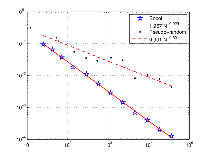
The following example shows a better convergence rate when using a low-discrepancy driver sequence rather than random point set. In each example the reported discrepancy for the AR algorithm using a random diver sequence is the average of independent runs, which is throughout all the numerical experiments.
Example 1.
In this example we consider a non-product target density in . Let target density be
Figure 2 shows the discrepancy by using deterministic points and pseudo-random points as driver sequence. For the RAR algorithm, we observe a convergence rate of , whereas the DAR algorithm shows a convergence rate of the discrepancy of order .

2.3 Deterministic algorithm for target density defined in real state space
Now we extend the domain of the target density to with . Assume that there is a proposal density function such that there exists a constant such that holds for all .
The inverse Rosenblatt transformation is used to generate samples from the proposal density in the real state space . Let be the joint CDF of and be the conditional CDF of the proposal density for . The transformation is used to generate points in from the unit cube , such that the projection of points onto the first coordinates has distribution . More precisely, let be the transformation given by
| (1) |
The first coordinates are produced by the inverse Rosenblatt transformation which converts the points from the unit cube into . The th coordinate is uniformly distributed on the line
if is uniformly distributed in . More details with respect to the Rosenblatt transformation and extensions can be found in [8, 29, 35].
Algorithm 3.
(Deterministic acceptance-rejection algorithm in ). Let an unnormalized target density function , where , be given. Let be a proposal density , such that there exists a constant such that for all . Let . Suppose we aim to obtain approximately samples from .
- i)
Let , where is the smallest integer satisfying this inequality. Generate a -net in base .
- ii)
Transform the points into from using the transformation given in (1) to obtain .
- iii)
Take the acceptance-rejection method for the sample with respect to and in , i.e. accept the point if , otherwise reject. Let .
- iv)
Project the points we accepted onto the first -dimensional space. Denote the first coordinates of the points we accept by the acceptance-rejection method by .
- v)
Return the point set .
We provide an example to demonstrate the performance of Algorithm 3.
Example 2.
Let the target density function be given by
The proposal density function , which we use to do the acceptance-rejection to generate samples of , is chosen as
For this choice of , we use transform defined in Equation (1) to obtain samples from . The sample is given by the following transformation
Note that is the driver sequence given by a -net in base .
The order of the star discrepancy is demonstrated in Figure 3 where is the number of accepted samples. The numerical experiments show that the star discrepancy converges at a rate of for this example using quasi-Monte Carlo samples as proposal. The RAR algorithm converges with order . Again, the DAR sampler outperforms the RAR sampler.

2.4 A deterministic reduced acceptance-rejection sampler
In this subsection we consider an extension of the DAR sampler. The random version of this reduced method was recently introduced by Barekat and Caflisch in [2]. For a target density function , we carefully select such that for and the inverse CDF can be computed. For the case , we write and get samples according to and respectively.
Figure 4 illustrates this method. The sample sets of can be divided into three subsets, and , where and can be directly generated by using the inverse CDF of and in a certain range. The acceptance-rejection method is only used to obtain . Compared with the ordinary acceptance-rejection sampler, one obvious merit of this method is that we do not require in the whole domain. Also, this method might give better convergence rates since and are obtained via inversion and therefore have low discrepancy. Algorithm 4 gives a simple version of the improved method. More discussion of a general version is available in Section 5.

Algorithm 4.
(Deterministic reduced acceptance-rejection (DRAR) algorithm) Let be a target density. Choose a proposal density such that and can be sampled directly. Let
| and | |||
Assume that and can be calculated or estimated. Let be the inverse CDF of the proposal density in the domain and respectively and be the inverse CDF with respect to in . Suppose we aim to generate approximately samples from . Let
- i)
Let be a -sequence in base .
- ii)
Use the acceptance-rejection method with the target density and the proposal density on the domain using as driver sequence. Choose such that points are accepted by the DAR algorithm. Compute for . Let be the accepted points. Label the point set as .
- iii)
Compute the points for . Let .
- iv)
Compute the points for . Let .
- v)
Project the points in onto the first coordinate. Return the point set .
Since the inverse transform is a measure-preserving transformation, it can preserve the uniformities of the driver sequence. Thus and are low discrepancy point sets. The following example verifies the efficiency of the DRAR algorithm. A theoretical result about the discrepancy properties of samples obtained by this class of algorithms is provided in Theorem 5.
Example 3.
Let be a density function defined on . Instead of seeking a proposal density such that , we notice that inversion can be implied to and independently. However, it can not work for their sum. Choose . We only do deterministic acceptance-rejection with respect to the target density and proposal density in the subinterval . In the remaining range , we apply the inverse transformation on and to obtain samples based on a deterministic driver sequence.
The discrepancy of the point set generated by Algorithm 4 converges at the rate of , which is significantly better than the convergence rate of a random driver sequence, see Figure 5.
3 Background on discrepancy theory and -nets
In this section we first establish some notation and some useful definitions and then obtain theoretical results. First we introduce the definition of -nets in base (see [11]) which we use as the driver sequence throughout the paper. The following fundamental definitions of elementary interval and fair sets are used to define a -net and -sequence in base .
Definition 1.
(b-adic elementary interval). Let be an integer. An -dimensional -adic elementary interval is an interval of the form
with integers and for all . If are such that , then we say that the elementary interval is of order .
Definition 2.
(fair sets). For a given set consisting of points in , we say for a subset of to be fair with respect to , if
where is the indicator function of the set and is the Lebesgue measure.
Definition 3.
(-nets in base b). For a given dimension , an integer base , a positive integer and an integer with , a point set of points in is called a -nets in base if the point set is fair with respect to all b-adic s-dimensional elementary intervals of order at most .
Definition 4.
(-sequence). For a given dimension , an integer base and a positive integer , a sequence of points in is called a -sequence in base if for all integers and , the point set consisting of the points forms a -net in base .
The concept of discrepancy is introduced in [16] to measure the deviation of a sequence from the uniform distribution. Now we give the definition of the so-called star discrepancy which enables us to distinguish the quality of point sets with respect to the uniform distribution.
Definition 5.
(star discrepancy). Let be a point set in . The star discrepancy is defined by
where the supremum is taken over all .
See Figure 6 for an illustration of the concept of discrepancy in the unit square.

If we extend the supremum in Definition 5 over all convex sets in , we get another interesting discrepancy, the so-called isotropic discrepancy. It is another measure of the distribution properties of point sets with respect to convex sets.
Definition 6.
(isotropic discrepancy). Let be a point set in . The isotropic discrepancy is defined to be
where is the family of all convex subsets of .
For further reading about the definition and properties of discrepancy, we refer for instance to [11, 16].
For our purposes here we need the definition of pseudo-convex sets which we introduce in the following (see also [1, Definition 2] and Figure 7 for an example).
Definition 7.
(pseudo-convex set). Let be an open subset of such that there exists a collection of convex subsets of satisfying
- 1.
for ;
- 2.
of ;
- 3.
either is a convex part of ( for ) or the complement of with respect to , is convex.
Then is called a pseudo-convex set and is an admissible convex covering for with parts and with convex parts of .

Remark 1.
For convenience, we call a nonnegative function pseudo-convex if and only if the region below its graph is a pseudo-convex set.
Next we present a bound on the isotropic discrepancy of points generated by -nets. A detailed proof is given in Appendix B.1.
Lemma 1.
Let the point set be a -net in base where . For the isotropic discrepancy of we have
Lemma 2.
For any point set in we have
Further it is known from [20] that the star discrepancy of a -net in base , where , satisfies
for some constant . These two inequalities therefore yield a convergence rate of order .
The following lemma will be used to get a discrepancy bound for a point set on a pseudo-convex set. It is an extension of [1, Lemma 5] to the unit cube.
Lemma 3.
Let be a pseudo-convex subset of with admissible convex covering of parts with convex parts of . Then for any point set we have
4 Discrepancy investigation of deterministic acceptance-rejection sampler
The first result we get is a discrepancy bound with respect to the target density of samples generated by the acceptance-rejection algorithm with deterministic driver sequences. The star discrepancy of points generated by the acceptance-rejection algorithm with respect to the target density converges at the rate of , where is the number of accepted samples. See Theorem 1 for details. The proof uses a bound on the discrepancy of our driver sequence with respect to convex sets (which is called isotropic discrepancy, see Definition 6 for details).
4.1 Upper bound
Let an unnormalized density function be pseudo-convex, and , but not necessarily . Assume that there exists a constant such that for all . Let the subset under the graph of be defined as
| (2) |
which is pseudo-convex in as is a pseudo-convex function. Assume that there is an admissible convex covering of with parts and with convex parts of . Without loss of generality, let be the convex subsets of and , such that is convex for .
The definition of the star discrepancy of a point set with respect to a density function is given as follows.
Definition 8.
Let be an unnormalized target density. Let be a point set in . The star discrepancy of with respect to the density is defined by
where and .
Remark 2.
Note that is a probability density function on . Thus the discrepancy in Definition 8 measures the difference between the distribution and the empirical distribution of the sample points with respect to the test sets for .
Theorem 1.
Let the unnormalized density function , with , be pseudo-convex. Assume that there is an admissible convex covering of given by Equation (2) with parts and with convex parts of . Then the discrepancy of the point set generated by Algorithm 2 using a -sequence in base , for large enough , satisfies
where and for all .
We postpone the proof of this theorem to Appendix B.1.
4.2 Lower bound
In this section, we provide a lower bound on the star discrepancy with respect to a convex density function. The general idea is to find, for a given driver point set, a density function satisfying a certain convergence rate.
Theorem 2.
Let be an arbitrary point set in . Then there exists a concave density function defined in such that, for samples generated by the acceptance-rejection algorithm with respect to and , we have
where is independent of and but depends on .
A detailed proof is provided in Appendix B.2. We would like to point out that the lower bound also limits the convergence rates which we can obtain in our current approach via convex sets. Note that a concave function is also pseudo-convex as defined in Remark 1.
Additionally, note that [3] (in dimension ) and [38] (for dimension ) showed the existence of points with discrepancy with respect to convex sets bounded from above by (where is a function of only ). This would yield an improvement of our results from to , however, those constructions are not explicit and can therefore not be used in computation.
4.3 Generalization to real state space
We consider now the case where the target density is defined on with . The aim is to show a discrepancy bound on samples generated by the deterministic acceptance-rejection method. The discrepancy with respect to a given density function is defined as follows.
Definition 9.
Let be a point set in . Let be an unnormalized probability density function. Then the star discrepancy is defined by
where and for .
We use the transformation given in Equation (1) to generate samples of . For the sake of investigating discrepancy, the following result is helpful. The lemma shows that the transformations and its inversion are both measure-preserving. For the proofs later, we assume that the proposal density is a product measure, i.e. , where is the marginal density with respect to . In our numerical examples, the proposal density is not necessarily of product type.
Lemma 4.
The transformation from the -dimensional unit cube to given in (1) is measure-preserving, i.e. holds for any measurable set . This is true for as well.
To prove a bound on the discrepancy of the samples generated by Algorithm 3, the following assumption is needed.
Assumption 1.
Let be the target density and be a product measure proposal density function, which is chosen such that its inverse CDF can be computed. Let and the transformation is defined as the inversion of transform . Then we assume that is pseudo-convex.
As the mappings and are measure preserving, and since there are the same number of samples in an arbitrary subset and the corresponding subset , we can consider the discrepancy in the unit cube instead of that in . Following by similar proof arguments as for Theorem 1 and Theorem 2, we obtain the same discrepancy bounds including an upper bound and a lower bound for the general density defined in the real state space .
Theorem 3.
Theorem 4.
Let be a product density function defined on . Let be the transformation given in Equation (1) associated to . Let be an arbitrary point set in , then is a point set in . Then there exists an unnormalization density function defined in satisfying the assumption in Theorem 3 such that the star discrepancy of the points generated by the acceptance-rejection sampler with respect to and satisfies
where is independent of and , but only dependent on .
5 Discrepancy properties of the deterministic reduced acceptance-rejection sampler
Algorithm 4 can be extended to a more general case. Consider the target density . If it is possible to sample from individually and the expectations of can be calculated or estimated with low cost, then we can use an embedding deterministic reduced acceptance-rejection sampler in each step. Let
| and | |||
where for , and, in particular, is the target density.
Suppose we aim to sample points from the target density . The sample set can be divided into two types, namely, points generated from the sets ’s and ’s respectively. We apply a deterministic acceptance-rejection method given in Algorithm 3 in each with respect to and . Note that we get points from for . For sampling from , the remaining samples come from applying the inverse transformation of in . Then we obtain additional points from for . We conduct the procedure inductively until we get samples from . We assume that and can be calculated or estimated.
The following algorithm is an extension of the DRAR algorithm, which summarizes the embedding idea.
Algorithm 5.
Let , be a target density we aim to sample from. Define for . Denote and like in Equation (5) and assume that and can be calculated or estimated. Further assume that we can sample from individually by applying the transformation and given in Equation (1) in and respectively. Suppose we aim to generate samples from . Let
For from 1 to do:
- i)
Let be a -sequence in base .
- ii)
Compute for . Use the acceptance-rejection method with respect to and on the domain using as driver sequence. Choose such that points are accepted by the DAR algorithm. Let be the accepted points.
- iii)
Compute for . Let .
Let and let denote the projection of onto the first coordinates. Return the set .
Now we consider the discrepancy properties of sample points produced by this algorithm. Note that the sample set of can be decomposed into several subsets with different star discrepancy.
Theorem 5.
For a given target density , let . Let and be given by (5). Let be the sample set generated by Algorithm 5, where
which is the number of points generated from , and
which is the number of points generated from for . Assume that and can be calculated or estimated for the given target density and . Then we have
where and is the discrepancy of the samples in and respectively.
The proof of Theorem 5 is given in Appendix B.3. Note that this method achieves an improved acceptance rate of points since we are only rejecting points in a certain range. For the remaining domain, we get samples by applying the inverse transform. To be more exact, all point sets from have low discrepancy since the inverse transformation is directly applied with respect to for . Now we consider the star discrepancy of points generated from .
The following result from [20] gives an improved upper bound on the star discrepancy on the first terms of a -sequence in base with .
Lemma 5.
The star discrepancy of the first terms of a -sequence in base with satisfies
for some constant only depending on .
With the help of Lemma 2, we obtain a bound on the isotropic discrepancy of the first points of a -sequence.
Lemma 6.
Let the point set be the first terms of a -sequence. For the isotropic discrepancy of we have
for some constant depending only on .
Hence, for the star discrepancy of for , using a -sequence as a diver sequence in the DAR algorithm we have a convergence rate of order . We omit a detailed proof since similar arguments as for proving Theorem 1 can be used. The following corollary holds by substituting the proper upper bounds and in terms of .
6 Conclusion and outlook
As is well known, the integration error using a Monte Carlo method converges at the rate of . The acceptance-rejection sampler with a deterministic driver sequence, which is a simple class of MCQMC methods, performs much better in our numerical experiments than the theoretical result of Theorem 1 or Theorem 3, for a density defined on or , would imply. The three examples even demonstrate that it is possible to achieve a better convergence rate than with standard Monte Carlo using a well-chosen deterministic driver sequence.
The main drawback of the acceptance-rejection sampler is that it might reject many points in high dimension. Some methods to improve the acceptance rate of points are included in [19]. For a special class of density functions given by a finite sum, we propose an embedding deterministic reduced acceptance-rejection algorithm. This algorithm produces a better star discrepancy convergence rate in our numerical example.
References
- [1] C. Aistleitner, J.S. Brauchart and J. Dick. Point Sets on the Sphere with Small Spherical Cap Discrepancy. Discrete and Computational Geometry, 48, 990–1024, 2012.
- [2] F. Barekat and R.Caflisch. Simulation with Fluctuation and Singular Rates. ArXiv:1310.4555[math.NA], 2013.
- [3] J. Beck. On the discrepancy of convex plane sets. Monatshefte Mathematik, 105, 91–106, 1988.
- [4] C. Botts, W. Hörmann and J. Leydold. Transformed density rejection with inflection points. Statistics and Computing, 23, 251–260, 2013.
- [5] R.E. Caflisch. Monte Carlo and quasi-Monte Carlo methods. Acta Numerica, 1–49, 1998.
- [6] S. Chen. Consistency and convergence rate of Markov chain quasi Monte Carlo with examples. PhD thesis, Stanford University, 2011.
- [7] S. Chen, J. Dick and A.B. Owen. Consistency of Markov chain quasi-Monte Carlo on continuous state spaces. Annals of Statistics, 39, 673–701, 2011.
- [8] N.N. Chentsov. Pseudorandom numbers for modelling Markov chains. Computational Mathematics and Mathematical Physics, 7, 218–233, 1967.
- [9] L. Devroye. Nonuniform random variate generation. Springer-Verlag, New York, 1986.
- [10] J. Dick, F, Kuo and I.H. Sloan. High dimensional integration-the Quasi-Monte Carlo way. Acta Numerica, 22, 133–288, 2013.
- [11] J. Dick and F. Pillichshammer. Digital Nets and Sequences. Discrepancy Theory and Quasi-Monte Carlo Integration. Cambridge University Press, Cambridge, 2010.
- [12] J. Dick, D. Rudolf and H. Zhu. Discrepancy bounds for uniformly ergodic Markov chain quasi-Monte Carlo. Available at arxiv.org/abs/1303.2423[stat.CO], submitted, 2013.
- [13] H. Faure. Discrépance de suites associées à un système de numération (en dimension ). Acta Arithmetica, 4, 337–351, 1982.
- [14] M. Gerber and N. Chopin. Sequential quasi-Monte Carlo. Available at arXiv:1402.4039 [stat.CO], 2014.
- [15] M. Gnewuch. Bracketing numbers for axis-parallel boxes and application to geometric discrepancy. Journal of Complexity, 24, 154–172, 2008.
- [16] L. Kuipers and H. Niederreiter. Uniform Distribution of Sequences. John Wiley, New York, 2006.
- [17] J.H. Halton. On the efficiency of certain quasi-random sequences of points in evaluating multi-dimensional integrals. Numerische Mathematik, 2, 84–90, 1960.
- [18] K. Hesse. A lower bound for the worst-case cubature error on spheres of arbitrary dimension. Numerische Mathematik, 103, 413–433, 2006.
- [19] W. Hörmann, J. Leydold and G. Derflinger. Automatic nonuniform random variate generation. Statistics and Computing. Springer-Verlag, Berlin, 2004.
- [20] P. Kritzer. Improved upper bounds on the star discrepancy of -nets and -sequences. Journal of Complexity, 22, 336–347, 2006.
- [21] P. L’Ecuyer, C. Lecot and B. Tuffin. A randomized quasi-Monte Carlo simulation method for Markov chains. Operation Research, 56, 958–975, 2008.
- [22] M.P. Meyn and T.L. Tweedie. Markov chain and stochastic stability. Springer-Verlag, London, 1993.
- [23] W.J. Morokoff and R.E. Caflisch. Quasi-Monte Carlo integration. Journal of Computational Physics, 122, 218–230, 1995.
- [24] B. Moskowitz and R.E. Caflisch. Smoothness and dimension reduction in quasi-Monte Carlo methods. Mathematical and Computer Modelling, 23, 37–54, 1996.
- [25] N. Nguyen and G. Ökten. The acceptance-rejection method for low discrepancy sequences. Submitted, 2014.
- [26] H. Niederreiter. Low-discrepancy and Low-dispersion sequences. Journal of Number Theory, 30, 51–70, 1988.
- [27] H. Niederreiter. Random Number Generation and Quasi-Monte Carlo Methods. SIAM, Philadelphia, Pennsylvania, 1992.
- [28] H. Niederreiter and J.M. Wills. Diskrepanz und Distanz von Maßen bezüglich konvexer und Jordanscher Mengen. (German) Mathematische Zeitschrift, 144, 125–134, 1975.
- [29] Y. Noh, K.K. Choi and L. Du. New Transformation of Dependent Input Variables Using Copula for RBDO. 7th World Congresses of Structural and Multidisciplinary Optimization COEX Seoul, Korea, 21–25 May 2007.
- [30] A.B. Owen. Randomly permuted -nets and -sequences. In: H. Niederreiter and P.J. Shiue (Eds.). Monte Carlo and quasi-Monte Carlo methods in scientific computing (Las Vegas, NV, 1994), 299–317, Lecture Notes in Statist., 106, Springer, New York, 1995.
- [31] A.B. Owen. Monte Carlo variance of scrambled net quadrature. SIAM Journal on Numerical Analysis, 34, 1884–1910, 1997.
- [32] A.B. Owen. Scrambled net variance for integrals of smooth functions. Annals of Statistics, 25, 1541–1562, 1997.
- [33] A.B. Owen. Monte Carlo theory, methods and examples (book draft). Available at http://www-stat.stanford.edu/ owen/mc/. Last accessed on 23 April 2014.
- [34] C. Robert and G. Casella. Monte Carlo Statistical Methods. Springer-Verlag, New York, second edition, 2004.
- [35] M. Rosenblatt. Remarks on a multivariate transformation. Annals of Mathematical Statistics, 23, 470–472, 1952.
- [36] W.M. Schmidt. Irregularities of distribution. Acta Arithmetica, 27, 385–396, 1975.
- [37] I.M. Sobol. Distribution of points in a cube and approximate evaluation of integrals. Akademija Nauk SSSR. Žurnal Vyčislitel’ noĭ Matematiki i Matematičeskoĭ Fiziki 7, 784–802, 1967 (in Russian); U.S.S.R Computational Mathematics and Mathematical Physics 7, 86–112, 1967 (in English).
- [38] W. Stute. Convergence rates for the isotrope discrepancy. Annals of Probability, 5, 707–723, 1977.
- [39] S.D. Tribble. Markov chain Monte Carlo algorithms using completely uniformly distributed driving sequences. PhD thesis, Stanford University, 2007.
- [40] S.D. Tribble and A.B. Owen. Constructions of weakly CUD sequences for MCMC. Electronic Journal of Statistics, 2, 634–660, 2008.
- [41] X. Wang. Quasi-Monte Carlo integration of characteristic functions and the rejection sampling method. Comupter Physics Communication, 123, 16–26, 1999.
- [42] X. Wang. Improving the rejection sampling method in quasi-Monte Carlo methods. Journal of Computational and Applied Mathematics, 114, 231–246, 2000.
- [43] A.D. Wyner. Capabilities of bounded discrepancy decoding. The Bell system technical journal, 44, 1061–1122, 1965.
Supplement
A -cover to approximate star discrepancy
Since it is computationally too expensive to compute the supremum in the definition of the star-discrepancy exactly for dimensions larger than one, we use a so-called -cover to estimate this supremum.
Definition 10.
Let be a probability space where and is the Borel -algebra defined on . Let be a set of test sets. A finite subset is called a -cover of with respect to if for every there are sets such that
and
The concept of -cover is motivated by the following result [15]. Assume that is a -cover of with respect to the distribution . For all , the following discrepancy inequality holds
In the experiments we choose to be the set of intervals , where runs through all points in the domain. For densities defined in , we set , which means that the -cover becomes finer as the number of samples increases, thus it can yield a more accurate approximation of the star discrepancy. For densities defined in , we choose -covers with respect to as where is the inverse marginal CDF with respect to the proposal density . Note that the approximation of the star-discrepancy is computationally expensive, thus our experiments only go up to several thousand sample points. However, the generation of samples using a -net is fast.
B Proofs
Before giving the proofs, we need some preparation.
Consider the following elementary intervals
| (4) |
with (where is an integer) for . The diagonal of has length and the volume is . Let be an arbitrary convex set in . Let denote the union of cubes fully contained in ,
| (5) |
Let denote the union of cubes having non-empty intersection with or its boundary ,
| (6) |
To illustrate the result we provide the following simple argument which yields a slightly weaker result. Based on the construction of , its diagonal length is . Then
where is the Euclidean norm. Then
Note that the outer surface area of a convex set in is bounded by the surface area of the unit cube , which is . Thus the Lebesgue measure of the set is bounded by the outer surface area times the diameter. Therefore
The result for follows by a similar discussion as the proof above.
Remark 3.
Note that in [28] it was also shown that the constant is best possible.
Now we extend the result in Lemma 7 to pseudo-convex sets.
Corollary 2.
Proof.
Let be an admissible convex covering of with parts. Without loss of generality, let be the convex subsets of and be such that is convex for . It can be shown that
| (7) |
The result for follows by a similar discussion. ∎
B.1 Proof of upper bound
Proof of Lemma 1.
Proof.
For the point set generated by a -net in base with , let . Let be an arbitrary convex set in . Consider the elementary interval given by Equation (4). For and given by (5) and (6), obviously, . The sets and are fair with respect to the net, that is
Then
and
By Lemma 7, we have
Thus we obtain
Since the bound holds for arbitrary convex sets, the proof is complete. ∎
Proof of Theorem 1.
Proof.
Let , where and . Since are the first coordinates of for , we have
Therefore
The right-hand side above is now bounded by
where we used the estimation and the fact that . Since is also pseudo-convex, it follows from Lemma 3 that we can bound the above expression by
In addition, , which means . Hence there is an such that for all . Thus for all . Further we have . Using Lemma 1 we obtain the bound
∎
B.2 Proof of lower bound
The following lemma provides information about the packing number of the northern hemisphere
where . The (closed) spherical cap with center and angular radius is defined by
The packing of considered here is constructed by identical spherical caps which are non-overlapping, that is, and with touch at most at their boundaries.
Lemma 8.
Let . For any there exist points on the northern hemisphere and an angular radius , with
such that the caps , , form a packing of the northern hemisphere. The positive constant depend only on the dimension .
The lemma is essentially well-known for spheres. The explicit proof is due to Wyner [43] and Hesse gives a summary in [18, Lemma 1]. A similar argument can be used for the hemisphere in our case.
Now we give the proof of Theorem 2 whose proof follows the argument from the proof of [36, Theorem 1].
Proof.
We may suppose . Let be the northern hemisphere defined above contained in , and let be the surface of . Let be a closed spherical cap on with spherical radius . The convex hull of is a solid spherical cap. For , is a continuous function of with
| (8) |
If is sufficiently large, there is a positive real number of such that a cap of spherical radius has
In view of (8), . We now pick as many pairwise disjoint caps with radius as possible, say . By Lemma 8, for large and hence small we have , hence
| (9) |
Given a sequence of numbers , with each either or , let consist of all which do not lie in a cap with . In other words, is obtained form by removing the solid caps for which .
Now the local discrepancy function defined by is additive, i.e. it satisfies
if . It follows easily that
We have
Hence for every , either or . Choose such that . Then
and either or has . In addition, is a convex set due to its construction.
B.3 Proof of Theorem 5
Proof.
In what follows we restrict our investigations to the case for simplicity, the general case can be proved by similar arguments. Let be the target density function. Assume that we can apply the inverse CDF on and to generate samples. Let
| and | |||
The final sample set is a superposition of the three subsets, and , see Figure 4. Define for . The number of the points in each subset is given by
Then there exists for such that
Therefore,
where is the star discrepancy of sample points in associated with and the same notation is also applied to and . Since this result holds for arbitrary , the desired result follows then immediately. ∎