Enumeration of chord diagrams on many intervals and their non-orientable analogsThanks: Research supported by the Centre for Quantum Geometry of Moduli Spaces which is funded by the Danish National Research Foundation. The work of NA and PZ was further supported by the Government of the Russian Federation megagrant 11.G34.31.0026, by JSC “Gazprom Neft”, and by the RFBR grants 13-01-00935-a and 13-01-12422-OFI-M2. In addition, NA was partially supported by the RFBR grant 14-01-00500-a and by the SPbSU grant 6.38.672.2013, and PZ was partially supported by the RFBR grant 14-01-00373-a

A partial chord diagram is a connected fatgraph (i.e., a graph equipped with a cyclic order on the half edges incident to each vertex) comprised of an ordered set of $b\geq 1$ disjoint real line segments (called backbones) connected with $k\geq 0$ chords in the upper half plane with distinct endpoints, so that there are $2k$ vertices of degree three (or chord endpoints) and $l\geq 0$ vertices of degree two (or marked points) all belonging to the backbones (in effect, ignoring the vertices of degree one arising from backbone endpoints.) If $l=0$ so there are no marked points, then we call the diagram a (complete) chord diagram. Each partial or complete chord diagram is a spine of an orientable surface with $n\geq 1$ boundary components and therefore has a well-defined topological genus. The genus $g$ of a partial chord diagram on $b$ backbones and its number $n$ of boundary components are related by Euler’s formula $b-k+n=2-2g$.

Chord diagrams occur pervasively in mathematics, which further highlights the importance of the counting results obtained here. To mention a few, see the theory of finite type invariants of knots and links [19] (cf. also [9]), the representation theory of Lie algebras [12], the geometry of moduli spaces of flat connections on surfaces [5, 6] and mapping class groups [2]. Moreover and as we shall further explain later, partial and complete chord diagrams each provide a useful model [28, 29, 25, 37] for the combinatorics of interacting RNA molecules with the associated genus filtration of utility in enumerative problems [3, 11, 25, 32, 33, 37, 38] and in folding algorithms on one [35, 10] and two backbones [4].

Our goal is to enumerate various classes of connected partial and complete chord diagrams, and to this end, we next introduce combinatorial parameters, where each enumerative problem turns out to be solved by an elegant partial differential equation on a suitable generating function in dual variables. In effect, creation and annihilation operators for the combinatorial data are given by multiplication and differentiation operators in the dual variables leading to algebraic differential equations.

We say that a partial chord diagram has

• •

  backbone spectrum $\boldsymbol{b}=(b_{1},b_{2},\ldots)$ if the diagram has $b_{i}$ backbones with precisely $i\geq 1$ vertices (of degree either two or three);

• •

  boundary point spectrum $\boldsymbol{n}=(n_{0},n_{1},\ldots)$ if its boundary contains $n_{i}$ connected components with $i$ marked points;

• •

  boundary length spectrum ${\boldsymbol{p}}=({p}_{1},{p}_{2},\ldots)$ if the boundary cycles of the diagram consist of ${p}_{i}$ edge-paths of length $i\geq 1$, where the length of a boundary cycle is the number of chords it traverses counted with multiplicity (as usual on the graph obtained from the diagram by collapsing each backbone to a distinct point) plus the number of backbone undersides it traverses (or in other words, the number of traversed backbone intervals obtained by removing all the chord endpoints from all the backbones).

The data $\{g,k,l;\boldsymbol{b};\boldsymbol{n};\boldsymbol{p}\}$ is called the type of a partial chord diagram (cf. Fig. 1). Note that the entries in the data set $\{g,k,l;\boldsymbol{b};\boldsymbol{n};\boldsymbol{p}\}$ are not independent. In particular, we have

Let $\mathcal{N}_{g,k,l}({\boldsymbol{b}},{\boldsymbol{n}},\boldsymbol{p})$ denote the number of distinct connected partial chord diagrams of type $\{g,k,l;{\boldsymbol{b}};{\boldsymbol{n}};\boldsymbol{p}\}$ taken to be zero if there are no chord diagrams of the specified type. Our two basic models involve boundary point spectra of partial chord diagrams and boundary length spectra of complete chord diagrams, and each basic model, in turn, has both an orientable and a non-orientable incarnation.

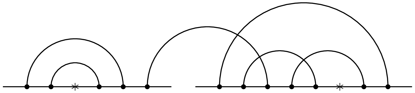
We may also consider non-orientable chord diagrams. Let $\widetilde{\mathcal{N}}_{h,k,l}(\boldsymbol{b},\boldsymbol{n},\boldsymbol{p})$ denote the number of both orientable and non-orientable connected diagrams on $b$ backbones, out of which exactly $b_{i}$ have $i$ vertices, with $k$ pairs of vertices connected by (twisted or untwisted) chords, with boundary point and boundary length spectra $\boldsymbol{n}$ and $\boldsymbol{p}$ respectively, and with Euler characteristic $2-h-n,\;n=\sum_{i=1}^{\infty}n_{i}$, where $h$ denotes twice the genus in the orientable case and the number of cross caps in the non-orientable case. This can evidently be formalized in the language of planar projections of chord diagrams by two-coloring the chords depending upon whether they preserve or reverse the orientation of the plane of projection.

For partial chord diagrams and boundary point spectra, we shall count the subsets

in the orientable case and

in the non-orientable case.

We can equivalently replace each backbone component containing $b_{i}$ vertices by a polygon with $b_{i}$ sides (one of which is distinguished, corresponding to the first along the backbone). Thus, the numbers $\mathcal{N}_{g,k,l}(\boldsymbol{b},\boldsymbol{n})$ count the orientable genus $g=1+(k-b-n)/2$ connected gluings of $b$ polygons, among which exactly $b_{i}$ have $i$ sides, with $k$ pairs of sides identified in such a way that the boundary of the glued surface has exactly $n_{i}$ connected components consisting of $i$ sides.¹¹ 1 For $b=1$, a similar problem was addressed in [1], but the formulas derived there are considerably different from the ones obtained in this paper and do not stand a numerical check. In particular, the Harer-Zagier numbers $\epsilon_{g,k}$ [15] that enumerate closed orientable genus $g$ gluings of a $2k$-gon coincide with the numbers $\mathcal{N}_{g,k,l}(\boldsymbol{n},\boldsymbol{b})$ with $\boldsymbol{n}=(k-2g+1,0,0,\dots)$ and $\boldsymbol{b}=\boldsymbol{e}_{2k}$, where we denote by $\boldsymbol{e}_{i}$ the vector with 1 in the $i$-th place and $0$ elsewhere.

A useful notation for exponentiating a $m$-tuple $\boldsymbol{a}=(a_{1},a_{2},\ldots,a_{m})$ of variables by an integral $m$-tuple $\boldsymbol{\alpha}=(\alpha_{1},\alpha_{2},\ldots,\alpha_{m})$ is to write simply ${\boldsymbol{a}}^{\boldsymbol{\alpha}}=a_{1}^{\alpha_{1}}a_{2}^{\alpha_{2}}\ldots a_{m}^{\alpha_{m}}$; we extend this notation in case $\boldsymbol{a}=(a_{1},a_{2},a_{3},\ldots)$ is a fixed infinite sequence of variables and $\boldsymbol{\alpha}$ is a finite tuple. In this notation and setting $\boldsymbol{s}=(s_{0},s_{1},\ldots)$ and $\boldsymbol{t}=(t_{1},t_{2},\ldots)$, we define the orientable, multi-backbone, boundary point spectrum generating function $F(x,y;\boldsymbol{s};\boldsymbol{t})=\sum_{b\geq 1}F_{b}(x,y;\boldsymbol{s};\boldsymbol{t})$, where

and the non-orientable generating functions $\tilde{F}(x,y;\boldsymbol{s};\boldsymbol{t})=\sum_{b\geq 1}\tilde{F}_{b}(x,y;\boldsymbol{s};\boldsymbol{t})$, where

(we recall that $2-2g=b-k+\sum_{i\geq 0}n_{i}$ in the orientable case and $2-h=b-k+\sum_{i\geq 0}n_{i}$ in the non-orientable case, while in the both cases $l=\sum_{i\geq 1}in_{i}$).

Equivalently, each differential equation is solved by exponentiating $k$ times the operator on the right hand side applied to $x^{-2}\sum_{i\geq 1}s_{i}t_{i}$, for example,

This explains the relationship between these differential equations and the corresponding enumerative problems. These are the most efficient enumerations of which we are aware. As we shall see in the proof, each term corresponds to adding a certain type of chord: $L_{0}$ and $L_{2}$, respectively, for chords with both endpoints on the same and different boundary components lying in a common component, $Q$ for chords whose removal separates the diagram, and $L_{1}$ the analogue of $L_{0}$ for Möbius bands that give rise to Möbius graphs as compared to fatgraphs in the oriented case (the subscripts 0,1 and 2 by $L$ reflect the change in the Euler characteristic of the chord diagram under such an operation).

In the last section of this paper, we provide matrix model formulas for certain linear combinations of the numbers $\mathcal{N}_{g,k,l}(\boldsymbol{b},\boldsymbol{n})$ and $\widetilde{\mathcal{N}}_{h,k,l}(\boldsymbol{b},\boldsymbol{n})$. This allows us to compare our computations for partial chord diagrams with results on a certain limiting spectral distribution, the so-called large $N$-limit for one backbone. Note that a recursion for the numbers $\widetilde{\mathcal{N}}_{h,k,0}({\boldsymbol{e}}_{2k},{\boldsymbol{n}})$, for ${\boldsymbol{n}}=(k-h+1,0,\dots),$ of all complete (not necessarily orientable) gluings of a $2k$-gon was derived in [21] using the methods of random matrix theory. Our formulas specialize to those of [21] in this particular case.

For complete chord diagrams and boundary length spectra, we shall count the subsets

in the orientable case and

in the non-orientable case. We define the orientable, multi-backbone, length spectrum generating function $G(x,y,t;\boldsymbol{s})=\sum_{b\geq 1}G_{b}(x,y;\boldsymbol{s})t^{b}$, where

and the non-orientable generating function $\tilde{G}(x,y,t;\boldsymbol{s})=\sum_{b\geq 1}\;\tilde{G}_{b}(x,y;\boldsymbol{s})t^{b}$, where

The following observation we learned from M. Kazarian [17, 18]: for $x=1$ the generating functions $F\left|{}_{x=1}\right.$ and $G\left|{}_{x=1}\right.$ satisfy an infinite system of non-linear partial differential equations called the KP (Kadomtsev-Petviashvili) hierarchy (in particular, this means that the numbers $\mathcal{N}_{g,k,l}(\boldsymbol{b},\boldsymbol{n})$ and ${\mathcal{N}}_{g,k,b}(\boldsymbol{p})$ additionally obey an infinite system of recursions). The KP hierarchy is one of the best studied completely integrable systems in mathematical physics. Below are the several first equations of the hierarchy:

where the subscript $i$ stands for the partial derivative with respect to $s_{i}$. The exponential $e^{F}$ of any solution is called a tau function of the hierarchy. The space of solutions (or the space of tau functions) has a nice geometric interpretation as an infinite-dimensional Grassmannian (called the Sato Grassmannian), see, e. g., [22] or [17] for details. See also [8] for another application of the Sato Grassmannian to conformal field theory. The space of solutions is homogeneous: there is a Lie algebra $\widehat{\mathfrak{gl}(\infty)}$ (a central extension of $\mathfrak{gl}(\infty)$) that acts infinitesimally on the space of solutions, and the action of the corresponding Lie group is transitive.

Introduce the standard bosonic creation-annihilation operators

and put

(the notation $:\!a_{i_{1}}\dots a_{i_{r}}\!\!:$ stands for the ordered product $a_{i_{\sigma(1)}}\dots a_{i_{\sigma(r)}}$, where $\sigma\in S_{r}$ is a permutation such that $i_{\sigma(1)}\geq\dots\geq i_{\sigma(r)}$).²² 2 The operator $M_{0}$ is the famous cut-and-join operator [14] used in the computation of Hurwitz numbers. All the operators $a_{i},\;\varLambda_{m},\;M_{m}$ belong to the Lie algebra $\widehat{\mathfrak{gl}(\infty)}$. Moreover, it is easy to check that

so that $L_{0}+L_{2}$ and $K_{0}+K_{2}$ also belong to $\widehat{\mathfrak{gl}(\infty)}$. Now we notice that the exponentials $e^{\sum s_{i}t_{i}}$ and $e^{ts_{1}}$ of the initial conditions in Theorems 1 and 2 both are KP tau functions for a trivial reason – their logarithms are linear in $s_{1},s_{2},\dots$ and therefore obviously satisfy the equations of KP hierarchy (10) for any values of the other parameters. Moreover, both $e^{L_{0}+L_{2}}$ and $e^{K_{0}+K_{2}}$ preserve the Sato Grassmannian and map KP tau functions to KP tau functions. Thus, $e^{F\left|{}_{x=1}\right.}=e^{L_{0}+L_{2}}e^{\sum_{i\geq 1}s_{i}t_{i}}$ and $e^{G\left|{}_{x=1}\right.}=e^{K_{0}+K_{2}}e^{ts_{1}}$ are KP tau function as well, and we get

Let us now comment on the relevance of the above results to describing the RNA interactions. Define $C_{g,b,k}=\sum_{\boldsymbol{p}}{\mathcal{N}}_{g,k,b}(\boldsymbol{p})$ to be the number of complete and connected chord diagrams of genus $g$ on $b$ ordered and oriented backbones with $k$ chords, so in particular, $C_{g,1,k}$ is the Harer-Zagier number $\epsilon_{g,k}$. These chord diagrams provide the basic model for a complex of interacting RNA molecules, one RNA molecule for each backbone and one chord for each Watson-Crick³³ 3 These are the allowed bonds G-C and A-U between nucleic acids. For the expert, let us emphasize that any other model including wobble G-U or further exotic base pairs is handled in exactly the same way with one chord for each allowed type of bond. bond between nucleic acids, where one demands that the chord endpoints respect the natural ordering⁴⁴ 4 From the so-called 5’ to 3’ end as determined by the chemical structure of the RNA. of the nucleic acids in each molecule, i.e, in each oriented backbone. It is very natural, as is the attention to connected chord diagrams in order to avoid separate molecular interactions. In reality, RNA folds according to a partial chord diagram, i.e., there are in practice unbonded nucleic acids.⁵⁵ 5 Typically, 50 to 80 percent of nucleic acids participate in Watson-Crick base pairs together with several percent exotic. On the other hand in an extreme example, roughly 50 percent are Watson-Crick and 40 percent exotic for ribosomal RNA.

Recall from [7] that a shape is a special connected and complete chord diagram which has no parallel chords, has a unique “rainbow” on each backbone, i.e., a chord whose endpoints are closer to the backbone endpoints than any other chord and no “1-chords” connecting vertices consecutive in a single backbone unless the 1-chord is a rainbow. In the very special (genus zero on one backbone) case, the single-chord diagram is permitted since the 1-chord is a rainbow, but in all other cases, there are no 1-chords, each backbone has a unique rainbow, and ${p}_{1}=0$, ${p}_{2}=b$. If a shape is not the special single-chord diagram and we remove its $b$ rainbows, then the resulting diagram has ${p}_{1}=0={p}_{2}$. Conversely, in a chord diagram with ${p}_{1}=0={p}_{2}$, no backbone has a rainbow, and $b$ rainbows can be added to produce a shape. Let $S_{g,b,k}$ denote the number of shapes of genus $g$ on $b$ backbones with $k$ chords.

Define the generating functions $C(x,y,t)=\sum_{g=0}^{\infty}\sum_{b=1}^{\infty}C_{g,b}(y)x^{2g-2}t^{b}$, with

and $S(x,y,t)=\sum_{g=0}^{\infty}\sum_{b=1}^{\infty}S_{g,b}(y)x^{2g-2}t^{b}$, with

It follows by construction that

and $S(x,y,t)=1+G(x,y,t;0,0,1,1,\ldots)$, so we have computed here both the complete chord diagrams $C_{g,b,k}$ and the shapes $S_{g,b,k}$⁶⁶ 6 Furthermore, the free energy $F_{g}(s,t)$ for the matrix model in [3] is given (up to a constant depending only on $g$ times $N^{2-2g}$) by our $G(N^{-1},t^{\frac{1}{2}},s;1,1,1...)$.. In fact [3], the generating functions for shapes and chord diagrams are algebraically related by

where $C_{0}(z)=\frac{1-\sqrt{1-4z}}{2z}$ is the Catalan generating function, the former equation expressing the formal power series $C_{g,b}(z)$ in terms of the polynomial $S_{g,b}(z)$. As a further interesting open problem, inspired by the results of this paper, we ask if there is a non-zero finite order differential operator in the variables $(x,y,t)$ which together with an initial condition determines $C(x,y,t)$?

One point about shapes is that standard combinatorial techniques allow their “inflation” to complete chord diagrams as indicated in the previous formulas, and furthermore, complete chord diagrams can likewise be inflated to partial chord diagrams, cf. [7, 34]. Another point is that shape inflation is well-suited to the accepted Ansatz for free energy and so provides efficient polynomial-time algorithms for computing minimum free energy RNA folds [35, 34] at least in the planar case. A further geometric point [7] is that shapes of genus $g$ on $b$ backbones are dual to cells in the Harer-Mumford-Strebel [36] or Penner [27] decomposition of Riemann’s moduli space of genus $g$ surfaces with $b$ boundary components provided $2g-2+b>0$.

As was already discussed, it is really partial chord diagrams that actually describe complexes of RNA molecules with its distillation first to complete chord diagrams and then to shapes. All three formulations of the combinatorics have thus been treated here, namely, shapes and complete chord diagrams by the previous formulas and partial chord diagrams by inflation or instead directly with our generating function in Theorem 1.

This paper is organized as follows. Section 2 contains basic combinatorial results on the boundary point spectra of chord diagrams on one backbone and derives the equation given before on $F_{1}$ (Proposition 2), and section 3 extends these results to include possibly separating edges and derives the equation given before on $F$ (Proposition 4). Boundary point spectra of non-orientable surfaces are discussed in Section 4, and the equations given before on $\tilde{F}_{1}$ and $\tilde{F}$ are derived (Proposition 5), so together Propositions 2-5 comprise Theorem 1. Section 5 is dedicated to boundary length spectra, and the situation is similar to boundary point spectra in that each counts data for each fatgraph boundary cycle. For this reason, the arguments are only sketched for boundary length spectra culminating in the equations from before on $G_{1}$, $G$, $\tilde{G}_{1}$ and $\tilde{G}$ (Theorem 2). Section 6 introduces a random matrix technique for partial chord diagrams and provides a matrix integral for boundary point spectra computations in both the orientable and non-orientable cases. Free probability techniques permit the computation of the large-N limit which reproduces computations based on the partial differential equations, providing a consistency check on the entire discussion.

As before, $\boldsymbol{e}_{i}$ denotes the sequence $(0,\dots,0,1,0,\dots)$ with 1 in the $i$-th place and 0 elsewhere. We say simply that a diagram is of type $\{g,k,l;\boldsymbol{b};\boldsymbol{n}\}$ if it is of type $\{g,k,l;\boldsymbol{b},\boldsymbol{n},\boldsymbol{p}\}$ for some $\boldsymbol{p}$ and let $\mathcal{N}_{g,k,l}(\boldsymbol{b},\boldsymbol{n})=0$ if there are no diagrams of type $\{g,k,l;\boldsymbol{b};\boldsymbol{n}\}$.

Let us proceed with the multibackbone case.

References

- [1] E . T. Akhmedov, S. Shakirov, Gluings of surfaces with polygonal boundaries, Funct. Anal. Appl., 43 (2009), 245–253.
- [2] J.E. Andersen, A. J. Bene, J.-B. Meilhan, R. C. Penner, Finite type invariants and fatgraphs, Adv. Math. 225 (2010), 2117–2161.
- [3] J. E. Andersen, L. O. Chekhov, R. C. Penner, C. M. Reidys, P. Sulkowski, Topological recursion for chord diagrams, RNA complexes, and cells in moduli spaces, Nucl. Phys. B, 866 (2013), 414 – 443.
- [4] J.E. Andersen, F.W.D. Huang, R.C. Penner, C.M. Reidys, Topology of RNA-RNA interaction structures, Jour. Comp. Biol., 19 (2012), 928 – 943.
- [5] J.E. Andersen, J. Mattes, N. Reshetikhin, The Poisson Structure on the Moduli Space of Flat Connections and Chord Diagrams, Topology 35 (1996), 1069–1083.
- [6] J.E. Andersen, J. Mattes, N. Reshetikhin, Quantization of the algebra of chord diagrams, Math. Proc. Camb. Phil. Soc. 124 (1998), 451–467.
- [7] J.E. Andersen, R.C. Penner, C.M. Reidys , M.S. Waterman, Topological classification and enumeration of RNA structures by genus, Jour. Math. Biol. DOI 10.1007/s00285-012-0594-x (2012), 1–18.
- [8] J. E. Andersen, K. Ueno, Abelian conformal field theory and determinant bundles. Internat. J. Math. 18, no. 8, (2007), 919–993.
- [9] D. Bar-Natan, On the Vassiliev knot invariants. Topology 34 (1995), 423–475.
- [10] M. Bon and H. Orland, TT2NE: A novel algorithm to predict RNA secondary structures with pseudoknots, Nucl. Acids Res. 41 (2010), 1895–1900.
- [11] M. Bon, G. Vernizzi, H. Orland, A. Zee, Topological classification of RNA structures. Jour. Mol. Biol. 379 (2008), 900–911.
- [12] R. Campoamor-Stursberg and V. O. Manturov, Invariant tensor formulas via chord diagrams, Jour. Math. Sci. 108 (2004), 3018–3029.
- [13] O. Dumitsrescu, M. Mulase, A. Sorkin, B. Safnuk, The spectral curve of the Eynard-Orantin recursion via the Laplace transform, Contemp. Math. 593 (2013) 263-316.
- [14] I. P. Goulden, D. M. Jackson, Transitive factorizations into transpositions and holomorphic mappings on the sphere, Proc. Amer. Math. Soc. 125 (1997), 51–60.
- [15] J. Harer and D. Zagier, The Euler characteristic of the moduli space of curves, Inv. Math. 85 (1986), 457–485
- [16] V.A. Kazakov, M. Staudacher, T. Wynter, Character expansion methods for matrix models of dually weighted graphs, Comm. Math. Phys. 177 (1996) 451–468.
- [17] M. Kazarian, KP hierarchy for Hodge integrals, Adv. Math. 221, 1–21 (2009).
- [18] M. Kazarian, Private communication (2013).
- [19] K. Kontsevich, Vassiliev’s knot invariants, Adv. Sov. Math. 16 (1993), 137–150.
- [20] S. K. Lando, A. K. Zvonkin, Graphs on surfaces and their applications, Encyclopaedia of Mathematical Sciences 141, Springer-Verlag, Berlin (2004).
- [21] M. Ledoux, A recursion formula for the moments of the Gaussian orthogonal ensemble, Ann. Inst. H. Poincare Prob. Stat. 45 (2009), 754–769.
- [22] T. Miwa, M. Jimbo, E. Date, Solitons: Differential equations, symmetries and infinite-dimensional algebras, Cambridge Tracts in Mathematics 135, Cambridge University Press, Cambridge (2000).
- [23] A. Morozov, Sh. Shakirov, Generation of matrix models by -operators, JHEP04(2009)064.
- [24] A. Nica, R. Speicher, Lectures on the combinatorics of free probability, London Math. Soc. Lecture Notes Series 335 Cambridge University Press (2006).
- [25] H. Orland and A. Zee, RNA folding and large N matrix theory, Nucl. Phys. B 620 (2002), 456-476.
- [26] A. V. Pastor, O. P. Rodionova, Some formulas for the number of gluings, Zapiski Nauchnykh Seminarov POMI 406 (2012), 117–156.
- [27] R. C. Penner, The decorated Teichmuller space of a punctured surface, Comm. Math. Phys. 113 (1987), 299–339.
- [28] R. C. Penner and M. S. Waterman, Spaces of RNA secondary structures, Adv. Math. 101 (1993), 31–49.
- [29] R. C. Penner, Cell decomposition and compactification of Riemann’s moduli space in decorated Teichmueller theory. In: N. Tongring and R. C. Penner (eds) Woodshole mathematics-perspectives in math and physics. World Scientific, Singapore, 263–301 (2004).
- [30] R. C. Penner, M. Knudsen, C. Wiu, J. E. Andersen, Fatgraph model of proteins, Comm. Pure Appl. Math. 63 (2010), 1249–1297.
- [31] R.C. Penner, M. Knudsen, C. Wiuf, J. E. Andersen, An Algebro-Topological Model of Protein Domain Structure, PLoS ONE 6 (2011), 1 – 14.
- [32] M. Pillsbury, H. Orland, A. Zee, Steepest descent calculation of RNA pseudoknots, Phys. Rev. E 72 (2010), 011911.
- [33] M. Pillsbury, J. A. Taylor, H. Orland, A. Zee, An algorithm for RNA pseudoknots, arXiv: cond-mat/0310505v2 (2005).
- [34] C. M. Reidys, Combinatorial and Computational Biology of Pseudoknot RNA, Applied Math series, Springer (2010).
- [35] C.M. Reidys, F.W.D. Huang, J.E. Andersen, R.C. Penner, P.F. Stadler, M. Nebel, Topology and prediction of RNA pseudoknots, Bioinf. 27 (2011) 1076–1085.
- [36] K. Strebel, Quadratic differentials, Ergebnisse der Mathematik und ihrer Grenzgebiete (3), 5. Springer-Verlag, Berlin (1984).
- [37] G. Vernizzi, H. Orland, A. Zee, Enumeration of RNA structures by matrix models. Phys. Rev. Lett. 94 (2005), 168103.
- [38] G. Vernizzi, P. Ribecca, H. Orland, A. Zee, Topology of pseudoknotted homopolymers, Phys. Rev. E 73 (2006), 031902.