跳到论文正文
W Papers独立论文阅读器 arXiv:1307.0888 论文正文 计算阅读时间 · 0%
引用这篇论文根据当前论文元数据生成,正式投稿前建议核对。


License: arXiv.org perpetual non-exclusive license
arXiv:1307.0888v2 [math.NA] 03 Sep 2013

Numerical Approximation of Fractional Powers of Elliptic Operators

Andrea Bonito Address: Department of Mathematics, Texas A&M University, College Station, TX 77843-3368. Email address: bonito@math.tamu.edu and Joseph E. Pasciak Address: Department of Mathematics, Texas A&M University, College Station, TX 77843-3368. Email address: pasciak@math.tamu.edu
Date: August 24, 2026
Abstract.

We present and study a novel numerical algorithm to approximate the action of Tβ:=L−βT^{\beta}:=L^{-\beta} where LL is a symmetric and positive definite unbounded operator on a Hilbert space H0H_{0}. The numerical method is based on a representation formula for T−βT^{-\beta} in terms of Bochner integrals involving (I+t2​L)−1(I+t^{2}L)^{-1} for t∈(0,∞)t\in(0,\infty).

To develop an approximation to TβT^{\beta}, we introduce a finite element approximation LhL_{h} to LL and base our approximation to TβT^{\beta} on Thβ:=Lh−βT_{h}^{\beta}:=L_{h}^{-\beta}. The direct evaluation of ThβT_{h}^{\beta} is extremely expensive as it involves expansion in the basis of eigenfunctions for LhL_{h}. The above mentioned representation formula holds for Th−βT_{h}^{-\beta} and we propose three quadrature approximations denoted generically by QhβQ_{h}^{\beta}. The two results of this paper bound the errors in the H0H_{0} inner product of Tβ−Thβ​πhT^{\beta}-T_{h}^{\beta}\pi_{h} and Thβ−QhβT_{h}^{\beta}-Q_{h}^{\beta} where πh\pi_{h} is the H0H_{0} orthogonal projection into the finite element space. We note that the evaluation of QhβQ_{h}^{\beta} involves application of (I+(ti)2​Lh)−1(I+(t_{i})^{2}L_{h})^{-1} with tit_{i} being either a quadrature point or its inverse. Efficient solution algorithms for these problems are available and the problems at different quadrature points can be straightforwardly solved in parallel. Numerical experiments illustrating the theoretical estimates are provided for both the quadrature error Thβ−QhβT_{h}^{\beta}-Q_{h}^{\beta} and the finite element error Tβ−Thβ​πhT^{\beta}-T_{h}^{\beta}\pi_{h}.

2010 Mathematics Subject Classification
35S15, 65R20, 65N12, 65N50, 65N30.

1. Introduction.

The mathematical study of integral or nonlocal operators has received much attention due to their wide range of applications, see for instance [8, 2, 11, 4, 19, 12, 25, 29, 9]. A prototype for such nonlocal operator results from the fractional powers of an elliptic operator and is the focus of this paper. A canonical example is given by Lβ=(I−Δ)βL^{\beta}=(I-\Delta)^{\beta} on ℝd{\mathbb{R}}^{d} and is naturally defined via Fourier transform, i.e.,

ℱ⁡(Lβ​f)​(ζ)=ℱ⁡((I−Δ)β​f)​(ζ)=(1+|ζ|2)β​ℱ​(f)​(ζ).{\mathcal{F}}(L^{\beta}f)(\zeta)={\mathcal{F}}((I-\Delta)^{\beta}f)(\zeta)=(1+|\zeta|^{2})^{\beta}{\mathcal{F}}(f)(\zeta).

Here ℱ⁡(v){\mathcal{F}}(v) denotes the Fourier transform of vv and β\beta is any real number.

We shall be concerned with similar problems, but posed on a bounded Lipschitz domain Ω\Omega. Specifically, given ff, we seek u=L−β​fu=L^{-\beta}f with β∈(0,1)\beta\in(0,1) and LL given by, for example, L=(I−Δ)L=(I-\Delta). In this case, we need to augment the problem with boundary conditions, e.g.,

(1) ∂u∂n\displaystyle\frac{\partial u}{\partial n} =0,on ΓN⊂∂Ω,\displaystyle=0,\qquad\hbox{on }\Gamma_{N}\subset\partial\Omega,
u\displaystyle u =0,on ΓD:=∂Ω∖ΓN.\displaystyle=0,\qquad\hbox{on }\Gamma_{D}:=\partial\Omega\setminus\Gamma_{N}.

Here nn denotes the outward pointing normal on ΓN\Gamma_{N}. When ΓD\Gamma_{D} has positive measure, we may also consider L=−ΔL=-\Delta.

We are concerned with the numerical approximation of u:=L−β​fu:=L^{-\beta}f. This problem has been studied by numerous authors [7, 14, 18, 16, 28, 21, 22, 31] (we give more details below). We note that L−βL^{-\beta} is defined in terms of the spectral decomposition of LL, i.e, u:=L−β​fu:=L^{-\beta}f is given by

(2) u⁡(x)=∑i=1∞λi−β​ci​ψi​(x).u(x)=\sum_{i=1}^{\infty}\lambda_{i}^{-\beta}c_{i}\psi_{i}(x).

Here cic_{i} are the Fourier coefficients of ff in the L2L_{2}-orthonormal basis {ψi​(x)}i=1∞\{\psi_{i}(x)\}_{i=1}^{\infty} of eigenfunctions for LL and {λi}i=1∞⊂ℝ+∖{0}\{\lambda_{i}\}_{i=1}^{\infty}\subset\mathbb{R}_{+}\setminus\{0\} are the respective eigenvalues.

There are several techniques for approximating L−β​fL^{-\beta}f in the literature. The most natural approach is to introduce a (finite dimensional) numerical approximation LhL_{h} of LL and obtain an approximation uh:=Lh−β​fu_{h}:=L^{-\beta}_{h}f using an expression similar to (2) but involving the eigenfunctions and eigenvalues of LhL_{h} [22, 21, 31]. The difficulty with this approach is that the direct evaluation of the resulting approximation is computationally very expensive. Indeed, it requires the computation of all eigenvectors and eigenvalues of a large system of linear equations. The purpose of this paper is to provide a more efficient technique for approximating uhu_{h} (and hence uu) which avoids the above mentioned eigenvalue/eigenvector computations.

An alternative approach for approximating u:=L−β​f:=(−Δ)−β​fu:=L^{-\beta}f:=(-\Delta)^{-\beta}f (or a more general elliptic partial differential equation) is based on a representation of uu via a “Neumann to Dirichlet” map [7]. Namely, uu is given, up to a normalization constant, by u⁡(x)=v⁡(x,0)u(x)=v(x,0) where v:Ω×ℝ+→ℝv:\Omega\times\mathbb{R}_{+}\rightarrow\mathbb{R} solves

−div(y1−2​β∇v(x,y))=0,(x,y)∈Ω×ℝ+-\textrm{div}(y^{1-2\beta}\nabla v(x,y))=0,\qquad(x,y)\in\Omega\times\mathbb{R}_{+}

together with the boundary conditions:

v⁡(⋅,y)​ satisfies\displaystyle v(\cdot,y)\hbox{ satisfies } (1) for each ​y∈ℝ+,\displaystyle\hbox{\eqref{e:bc} for each }y\in\mathbb{R}_{+},
limy→∞v⁡(x,y)\displaystyle\lim_{y\rightarrow\infty}v(x,y) =0,x∈Ω,\displaystyle=0,\quad x\in\Omega,
limy→0+(−y1−2​β​vy​(xCLOSECLOSE\displaystyle\lim_{y\to 0^{+}}\big(-y^{1-2\beta}v_{y}(x ,y))=f(x),x∈Ω.\displaystyle,y)\big)=f(x),\quad x\in\Omega.

The above equations leads to a well posed variational problem in an appropriately weighted Sobolev space [28] which is amendable to finite element approximation. The numerical algorithm proposed and analyzed in [28] consists of a ℝd+1\mathbb{R}^{d+1} finite element method which takes advantage of the rapid decay of the solution vv in the yy direction enabling truncation to a bounded domain of modest size. Error estimates are derived in a weighted H1​(Ω)H^{1}(\Omega)-norm.

Another natural approach for representing u:=L−β​fu:=L^{-\beta}f is via the Dunford Taylor integral, i.e.,

(3) u=12​π​i​(∫γz−β​Rz​(L)​𝑑z)​f.u=\frac{1}{2\pi i}\bigg(\int_{\gamma}z^{-\beta}R_{z}(L)\,dz\bigg)f.

Here γ\gamma is a positively oriented simple closed curve (in the extended complex plane) enclosing the spectrum of LL and Rz​(L)=(z​I−L)−1R_{z}(L)=(zI-L)^{-1} is the resolvent. A quadrature approximation of the above integral is proposed in [16]. In fact, the quadrature proposed in [16] but based on the hyperbolic path given in [17] leads to an exponentially convergent quadrature approximation. Our third scheme below is an example of another exponentially convergent quadrature but, in our case, only involves multiple evaluations of (I+ti​L)−1​f(I+t_{i}L)^{-1}f where ti∈(0,∞)t_{i}\in(0,\infty) is related to the quadrature node. There are numerous other papers proposing exponentially convergent quadrature schemes for Dunford-Taylor integral representations of e−t​Le^{-tL}, e.g., [26, 15, 16].

The algorithm developed here is also based on an integral representation of u=L−β​fu=L^{-\beta}f:

(4) L−β\displaystyle L^{-\beta} =2​sin⁡(π​β)π​[∫0∞t2​β−1​(I+t2​L)−1​𝑑t]\displaystyle=\frac{2\sin(\pi\beta)}{\pi}\bigg[\int_{0}^{\infty}t^{2\beta-1}(I+t^{2}L)^{-1}\ dt\bigg]
=2​sin⁡(π​β)π​[∫01t2​β−1​(I+t2​L)−1​dt+∫01t1−2​β​(t2​I+L)−1​dt],\displaystyle=\frac{2\sin(\pi\beta)}{\pi}\bigg[\int_{0}^{1}t^{2\beta-1}(I+t^{2}L)^{-1}\ dt+\int_{0}^{1}t^{1-2\beta}(t^{2}I+L)^{-1}\ dt\bigg],

We derive this identity in Section 2 from an identity in [3] (see, also [5, Chapter 10.4] and [32, Chapter 9.11]).

We develop and analyze two different quadrature schemes for the last two integrals above and a third for the first expression on the right of (4) under the transformation y=ln⁡(t)y=\ln(t), i.e.,

(5) L−β=2​sin⁡(π​β)π​[∫−∞∞e2​β​y​(I+e2​y​L)−1​𝑑y].L^{-\beta}=\frac{2\sin(\pi\beta)}{\pi}\bigg[\int_{-\infty}^{\infty}e^{2\beta y}(I+e^{2y}L)^{-1}\ dy\bigg].

The first quadrature is based on a β\beta-dependent graded mesh of NN subintervals per integral and a one point (rectangle) quadrature on each subinterval. Theorem 3.5 shows that there exists a constant C1C_{1} only depending on β\beta and the smallest eigenvalue of LL such that

(6) ‖(Lh−β−𝒬R,hβ)​f‖L2​(Ω)≤C1​N−1​‖f‖L2​(Ω),\|(L_{h}^{-\beta}-{\mathcal{Q}}_{R,h}^{\beta})f\|_{L^{2}(\Omega)}\leq C_{1}N^{-1}\|f\|_{L^{2}(\Omega)},

where 𝒬R,hβ{\mathcal{Q}}_{R,h}^{\beta} is the rectangle quadrature approximation to (4) with LL replaced by LhL_{h}, a finite dimensional approximation of LL. The second quadrature method starts with a dyadic partition of the interval [0,1][0,1]. Each subinterval is further decomposed in NN intervals of the same length on which a rr point weighted Gaussian quadrature is applied. Overall, this quadrature algorithm uses a number of quadrature points proportional to r2​N​ln⁡Nr^{2}N\ln N points. Theorem 3.5 shows that there exists a constant C2C_{2} only depending on β\beta and the smallest eigenvalue of LL such that

(7) ‖(Lh−β−𝒬G,hβ)​f‖L2​(Ω)≤C2​N−2​r​‖f‖L2​(Ω).\|(L_{h}^{-\beta}-{\mathcal{Q}}_{G,h}^{\beta})f\|_{L^{2}(\Omega)}\leq C_{2}N^{-2r}\|f\|_{L^{2}(\Omega)}.

Here 𝒬G,hβ{\mathcal{Q}}_{G,h}^{\beta} is the Gaussian quadrature approximation of (4) with LL replaced by LhL_{h}. The final quadrature involves 2​N+12N+1 equally spaced points applied to the integral (5) with a mesh size k=1/Nk=1/\sqrt{N} and yields an approximation 𝒬E,hβ{\mathcal{Q}}_{E,h}^{\beta} satisfying

(8) ∥(Lh−β−𝒬E,hβ)f∥L2​(Ω)≤C3e−c4/k∥f∥L2​(Ω).\|(L_{h}^{-\beta}-{\mathcal{Q}}_{E,h}^{\beta})f\|_{L^{2}(\Omega)}\leq C_{3}e^{-c_{4}/k}\|f\|_{L^{2}(\Omega)}.

Here C3C_{3} is a constant only depending on β\beta and the smallest eigenvalue of LL and c4c_{4} is an absolute constant. In what follows we denote 𝒬R,hβ{\mathcal{Q}}_{R,h}^{\beta}, 𝒬G,hβ{\mathcal{Q}}_{G,h}^{\beta} or 𝒬E,hβ{\mathcal{Q}}_{E,h}^{\beta} generically by 𝒬hβ{\mathcal{Q}}_{h}^{\beta}.

The final result provides estimates for ‖(L−β−Lh−β)​f‖L2​(Ω)\|(L^{-\beta}-L_{h}^{-\beta})f\|_{L^{2}(\Omega)} when Lh−1​fL_{h}^{-1}f is a finite element approximation of L−1​fL^{-1}f. These estimates depend on the elliptic regularity index 0<α≤10<\alpha\leq 1 (see conditions (c) and (d) of Section 4), e.g., α=1\alpha=1 when Ω\Omega is convex, the coefficients of LL are smooth and ΓD=∅\Gamma_{D}=\emptyset or ΓN=∅\Gamma_{N}=\emptyset. Theorem 4.3 shows that under these conditions, there exists a constant C5C_{5} uniform in hh and such that

(9) ‖(L−β−Lh−β​πh)​f‖L2​(Ω)\displaystyle\|(L^{-\beta}-L_{h}^{-\beta}\pi_{h})f\|_{L_{2}(\Omega)} ≤C5h2​αln(1/h)or\displaystyle\leq C_{5}h^{2\alpha}\ln(1/h)\quad\hbox{or}
‖(L−β−Lh−β​πh)​f‖L2​(Ω)\displaystyle\|(L^{-\beta}-L_{h}^{-\beta}\pi_{h})f\|_{L_{2}(\Omega)} ≤C5​h2​α\displaystyle\leq C_{5}h^{2\alpha}

depending on the smoothness of ff. Here πh\pi_{h} is now the L2​(Ω)L^{2}(\Omega) projection onto the finite element subspace. Combining (6), (7) or (8) with (9) provides an estimate for the difference between L−β​fL^{-\beta}f and its numerical approximation Qhβ​fQ_{h}^{\beta}f (see Corollary 4.4). Although the second result of (9) is well known when α=1\alpha=1 and h2​αh^{2\alpha} is replaced by h2​βh^{2\beta} (see [13] and Remark 4.3), we believe that our optimal order results are not available.

The computation of Qhβ​fQ_{h}^{\beta}f involves multiple independent evaluations of (I+(ti)2​Lh)−1​f\big(I+\big(t_{i}\big)^{2}L_{h}\big)^{-1}f with ti∈(0,∞)t_{i}\in(0,\infty) which can be implemented trivially in parallel. These are just finite element approximations to the problem (I+(ti)2​L)​w=f\big(I+\big(t_{i}\big)^{2}L\big)w=f (argumented with boundary conditions) and hence their implementation is classical. Moreover, multigrid preconditioners are available whose convergence rates can be guaranteed to be bounded independently of the parameters tit_{i} and hh.

For most of this work, we provide our analysis in a more general framework, namely, we assume that we are given two Hilbert spaces H1⊂H0H^{1}\subset H^{0} with H1H^{1} compactly, continuously and densely embedded in H0H^{0}. Denoting H−1H^{-1} and (H0)′(H^{0})^{\prime} to be the respective duals leads to an operator T:H−1→H1T:H^{-1}\rightarrow H^{1} (its inverse is LL in the above discussion). The usual identification H1⊂H0≅(H0)′⊂H−1H^{1}\subset H^{0}\cong(H^{0})^{\prime}\subset H^{-1} enables the definition of TβT^{\beta} (see Section 2 for the precise setting). This more general setting contains a large class of operators TT, for example, the inverse of the Laplace-Beltrami operator defined over Riemannian surfaces.

The outline of the remainder of the paper is as follows. In the next section, we motivate the integral identity (4). Section 3 defines our three numerical integration schemes for the scalar version of (4) (see (17)) and provides bounds for the quadrature error. The main result of this section is Theorem 3.2. This theorem is also illustrated by numerical experiments. The space discretization is developed in Section 4 for general elliptic operators. Theorem 4.3 provides the a-priori error estimate (9). The theoretical results are again followed by numerical illustration.

2. Integral Representation of Fractional Powers

We consider two Hilbert spaces H1H^{1} and H0H^{0} with inner products and norms, ⟨⋅,⋅⟩i\langle\cdot,\cdot\rangle_{i} and ∥⋅∥i\|\cdot\|_{i}, i=0,1i=0,1, respectively, and make the following two assumptions:

  1. (a)

    H1H^{1} is compactly and densely contained in H0H^{0}.

  2. (b)

    There is a constant c0c_{0} satisfying

    (10) ‖u‖0≤c0​‖u‖1,for all ​u∈H1.\|u\|_{0}\leq c_{0}\|u\|_{1},\qquad\hbox{for all }u\in H^{1}.

Let H−1H^{-1} denote the dual space of H1H^{1} with norm

‖F‖−1=supϕ∈H1⟨F,ϕ⟩‖ϕ‖1,\|F\|_{-1}=\sup_{\phi\in H^{1}}\frac{\langle F,\phi\rangle}{\|\phi\|_{1}},

where ⟨⋅,⋅⟩\langle\cdot,\cdot\rangle denotes the duality pairing. We define T:H−1→H1T:H^{-1}\rightarrow H^{1} by T​F:=uTF:=u where for F∈H−1F\in H^{-1}, T​F∈H1TF\in H^{1} is the unique solution of

⟨T​F,ϕ⟩1=⟨F,ϕ⟩,for all ​ϕ∈H1.\langle TF,\phi\rangle_{1}=\langle F,\phi\rangle,\qquad\hbox{for all }\phi\in H^{1}.

It is clear that TT is a isomorphism of H−1H^{-1} onto H1H^{1} and we denote LL to be its inverse. We define

D⁡(L):={v∈H0:L​v∈H0}.D(L):=\{v\in H^{0}\ :\ Lv\in H^{0}\}.

Our goal is to use (4) to approximate the fractional powers of TT, specifically, Tβ​f:=L−β​fT^{\beta}f:=L^{-\beta}f for 0<β<10<\beta<1 and f∈H0f\in H^{0}. For convenience we rewrite these integrals as

(11) Tβ\displaystyle T^{\beta} =Cβ−1​∫0∞t2​β−1​T1​(t)​𝑑t\displaystyle=C_{\beta}^{-1}\int_{0}^{\infty}t^{2\beta-1}\,T_{1}(t)\ dt
=Cβ−1​[∫01t2​β−1​T1​(t)​𝑑t+∫01t1−2​β​T2​(t)​𝑑t]\displaystyle=C_{\beta}^{-1}\bigg[\int_{0}^{1}t^{2\beta-1}\,T_{1}(t)\ dt+\int_{0}^{1}t^{1-2\beta}\,T_{2}(t)\ dt\bigg]

with

(12) Cβ:=∫0∞t2​β−1​(1+t2)−1​𝑑t=π2​sin⁡(π​β)C_{\beta}:=\int_{0}^{\infty}t^{2\beta-1}(1+t^{2})^{-1}dt=\frac{\pi}{2\sin(\pi\beta)}

(The last equality can be verified using the Beta function and the Euler reflexion formula). Here T2​(t):=t−2​T1​(t−1)T_{2}(t):=t^{-2}T_{1}(t^{-1}) and T1​(t):H−1→H1T_{1}(t):H^{-1}\rightarrow H^{1} is defined by T1​(t)​F:=uT_{1}(t)F:=u with u∈H1u\in H^{1} solving

(13) ⟨u,ϕ⟩0+t2​⟨u,ϕ⟩1=⟨F,ϕ⟩,for all ​ϕ∈H1.\langle u,\phi\rangle_{0}+t^{2}\langle u,\phi\rangle_{1}=\langle F,\phi\rangle,\qquad\hbox{for all }\phi\in H^{1}.

As usual, the function f∈H0f\in H^{0} is identified with the functional F∈H−1F\in H^{-1} is defined by ⟨F,ϕ⟩=⟨f,ϕ⟩0\langle F,\phi\rangle=\langle f,\phi\rangle_{0}, for all ϕ∈H1\phi\in H^{1}. We view (11) as an equality between elements of B⁡(H0,H0)B(H^{0},H^{0}), the set of bounded operators on H0H^{0}.

We note that

(14) ‖T1​(t)​f‖0≤‖f‖0\|T_{1}(t)f\|_{0}\leq\|f\|_{0}

follows immediately from (13). As u:=T2​(t)​fu:=T_{2}(t)f is the solution of

t2​⟨u,ϕ⟩0+⟨u,ϕ⟩1=⟨f,ϕ⟩0,for all ​ϕ∈H1,t^{2}\langle u,\phi\rangle_{0}+\langle u,\phi\rangle_{1}=\langle f,\phi\rangle_{0},\qquad\hbox{for all }\phi\in H^{1},

we have from (10) that

‖u‖0≤c0​‖u‖1≤c0​‖f‖−1.\|u\|_{0}\leq c_{0}\|u\|_{1}\leq c_{0}\|f\|_{-1}.

It follows, invoking (10) again, that for f∈H0f\in H^{0},

(15) ‖f‖−1≤c0​‖f‖0\|f\|_{-1}\leq c_{0}\|f\|_{0}

and hence

(16) ‖T2​(t)​f‖0=‖u‖0≤c02​‖f‖0.\|T_{2}(t)f\|_{0}=\|u\|_{0}\leq c_{0}^{2}\|f\|_{0}.

To make sense out of (11), we derive additional properties of TT. The compactness of H1H^{1} in H0H^{0} and (15) immediately imply that T:H−1→H−1T:H^{-1}\rightarrow H^{-1} is compact. Moreover, the norm on H−1H^{-1} comes from the inner product

⟨F,G⟩−1=⟨F,T​G⟩,for all ​F,G∈H−1\langle F,G\rangle_{-1}=\langle F,TG\rangle,\qquad\hbox{for all }F,G\in H^{-1}

from which it immediately follows that TT is a symmetric and positive definite operator on H−1H^{-1}. Fredholm theory implies that there is an ⟨⋅,⋅⟩−1\langle\cdot,\cdot\rangle_{-1} orthonormal basis of eigenfunctions {ψi}\{\psi_{i}\}, i=1,2,…i=1,2,\ldots for H−1H^{-1}. The corresponding (real) eigenvalues {μi}\{\mu_{i}\} are positive and, along with their eigenvectors, can be reordered to be non-increasing with limit 0. Given F∈H−1F\in H^{-1}, we define

Tβ​F:=∑i=1∞μiβ​⟨F,ψi⟩−1​ψi.T^{\beta}F:=\sum_{i=1}^{\infty}\mu_{i}^{\beta}\,\langle F,\psi_{i}\rangle_{-1}\,\psi_{i}.

The functions ψ~i=μi1/2​ψi{\widetilde{\psi}}_{i}=\mu_{i}^{1/2}\psi_{i}, i=1,2,…i=1,2,\ldots, provide an orthonormal basis for H0H^{0} (see Proposition 4.1 below) so that

Tβ​f=∑i=1∞μβ​⟨f,ψ~i⟩0​ψ~i,for all ​f∈H0.T^{\beta}f=\sum_{i=1}^{\infty}\mu^{\beta}\,\langle f,{\widetilde{\psi}}_{i}\rangle_{0}\,{\widetilde{\psi}}_{i},\qquad\hbox{for all }f\in H^{0}.

Moreover,

D⁡(L):={u∈H0:L​u∈H0}={u∈H0:∑i=1∞μi−2​⟨u,ψ~i⟩0<∞}.D(L):=\{u\in H^{0}\ :\ Lu\in H^{0}\}=\{u\in H^{0}\ :\ \sum_{i=1}^{\infty}\mu_{i}^{-2}\langle u,{\widetilde{\psi}}_{i}\rangle_{0}<\infty\}.

This implies that LL is a closed operator on H0H^{0} with domain D⁡(L)D(L) and that the range of LL on D⁡(L)D(L) coincides with H0H^{0}. We then have the following theorem.

Theorem 2.1.

Assume that H1H^{1} and H0H^{0} are Hilbert spaces satisfying (a) and (b). Then for 0<β<10<\beta<1, the integrals appearing in (11) are Bochner integrable and the equalities hold in B⁡(H0,H0)B(H^{0},H^{0}).

Proof.

We note that if z=(λ+L)−1​xz=(\lambda+L)^{-1}x for λ>0\lambda>0 and x∈H0x\in H^{0},

‖z‖0≤λ−1​‖x‖0.\|z\|_{0}\leq\lambda^{-1}\|x\|_{0}.

This implies (cf. [3], [5, Chapter 10.4] and [32, Chapter 9.11]) that for α∈(0,1)\alpha\in(0,1) and x∈D⁡(L)x\in D(L), the following is a well defined Bochner integral and satisfies

sin⁡(α​π)π​∫0∞λα−1​(λ​I+L)−1​L​x​𝑑λ=Lα​x.\frac{\sin(\alpha\pi)}{\pi}\int_{0}^{\infty}\lambda^{\alpha-1}(\lambda I+L)^{-1}Lx\ d\lambda=L^{\alpha}x.

Let β\beta be in (0,1)(0,1). Applying the above identity with α=1−β\alpha=1-\beta gives

L−β​y=sin⁡(α​π)π​∫0∞λα−1​(λ​I+L)−1​y​𝑑λL^{-\beta}y=\frac{\sin(\alpha\pi)}{\pi}\int_{0}^{\infty}\lambda^{\alpha-1}(\lambda I+L)^{-1}y\ d\lambda

for all yy in the range of LL, i.e., all y∈H0y\in H^{0}. Making the change of variable t2=λ−1t^{2}=\lambda^{-1} gives the first identity in (11). Breaking the first integral of (11) into two integrals on (0,1)(0,1) and (1,∞)(1,\infty), respectively, and making the change of variables t→t−1t\rightarrow t^{-1} in the second gives the second expression of (11). ∎

Remark 2.1.

We note that (16) is equivalent to

‖T1​(t)​f‖0≤(c0/t)2​‖f‖.\|T_{1}(t)f\|_{0}\leq(c_{0}/t)^{2}\|f\|.

Using this, (14) and (16), it readily follow that the integrals appearing in (11) are all well defined Bochner integrals.

Remark 2.2.

It is possible to extend these results to obtain negative powers of coercive (non-symmetric) bilinear forms but this extension is beyond the scope of the present paper.

3. Numerical Integration.

The numerical approximation to the integrals appearing in (11) is based on quadrature approximations to the scalar integrals:

(17) I⁡(λ)\displaystyle I(\lambda) =∫0∞t2​β−1​(1+t2​λ)−1​𝑑t\displaystyle=\int_{0}^{\infty}t^{2\beta-1}(1+t^{2}\lambda)^{-1}dt
=∫01t2​β−1​(1+t2​λ)−1​dt+∫01t1−2​β​(t2+λ)−1​dt=:I1​(λ)+I2​(λ).\displaystyle=\int_{0}^{1}t^{2\beta-1}(1+t^{2}\lambda)^{-1}dt+\int_{0}^{1}t^{1-2\beta}(t^{2}+\lambda)^{-1}dt=:I_{1}(\lambda)+I_{2}(\lambda).

In the next sections, we develop and analyze three quadratures.

For latter reference, we define

fλ​(t)≡fλ1​(t):=(1+λ​t2)−1,andfλ2​(t):=(t2+λ)−1.f_{\lambda}(t)\equiv f^{1}_{\lambda}(t):=(1+\lambda t^{2})^{-1},\qquad\text{and}\qquad f^{2}_{\lambda}(t):=(t^{2}+\lambda)^{-1}.

3.1. Rectangle quadrature rule on graded partitions

We start with I1​(λ)I_{1}(\lambda). We propose a graded partition of [0,1][0,1] to cope with the singular behavior of t2​β−1t^{2\beta-1} coupled with a one point quadrature. For a given positive integer NN, we set

  1. (i)

    t1,iN:=(i/N)12​βt^{N}_{1,i}:=(i/N)^{\frac{1}{2\beta}} if 2​β−1<02\beta-1<0.

  2. (ii)

    t1,iN:=i/Nt^{N}_{1,i}:=i/N if 2​β−1≥02\beta-1\geq 0.

Case (i) above corresponds to refinement at t=0t=0 and is necessary to deal with the singularity of the integrand at zero. We note that it is possible to use the node formula of Case (i) even when 2​β−1>02\beta-1>0. This results in larger spacing of the nodes near t=0t=0 compared to the uniform case and appears to be unnecessary.

The quadrature formula approximating I1​(λ)I_{1}(\lambda) reads

(18) I1N​(λ):=∑i=0N−1fλ1​(t1,iN,∗)​∫t1,iNt1,i+1Nt2​β−1=∑i=0N−1(t1,i+1N)2​β−(t1,iN)2​β2​β​fλ1​(t1,iN,∗).I_{1}^{N}(\lambda):=\sum_{i=0}^{N-1}f^{1}_{\lambda}\big(t_{1,i}^{N,*}\big)\int_{t_{1,i}^{N}}^{t_{1,i+1}^{N}}t^{2\beta-1}=\sum_{i=0}^{N-1}\frac{\big(t_{1,i+1}^{N}\big)^{2\beta}-\big(t_{1,i}^{N}\big)^{2\beta}}{2\beta}f^{1}_{\lambda}\big(t_{1,i}^{N,*}\big).

Here t1,iN,∗t_{1,i}^{N,*} is any point in the interval (t1,iN,t1,i+1N](t_{1,i}^{N},t_{1,i+1}^{N}]. In Case (i), the coefficient on the rightmost sum of (18) simplifies to (2​β​N)−1(2\beta N)^{-1}.

We proceed similarly for I2​(λ)I_{2}(\lambda). In this case, the partitioning is given by

  1. (iii)

    t2,iN:=(i/N)12−2​βt^{N}_{2,i}:=(i/N)^{\frac{1}{2-2\beta}} if 1−2​β<01-2\beta<0.

  2. (iv)

    t2,iN:=i/Nt^{N}_{2,i}:=i/N if 1−2​β≥01-2\beta\geq 0.

We define

(19) I2N​(λ):\displaystyle I_{2}^{N}(\lambda): =∑i=0N−1fλ2​(t2,iN,∗)​∫t2,iNt2,i+1Nt1−2​β\displaystyle=\sum_{i=0}^{N-1}f^{2}_{\lambda}(t_{2,i}^{N,*})\int_{t_{2,i}^{N}}^{t_{2,i+1}^{N}}t^{1-2\beta}
=∑i=0N−1(t2,i+1N)2−2​β−(t2,iN)2−2​β2−2​β​fλ2​(t2,iN,∗).\displaystyle=\sum_{i=0}^{N-1}\frac{\big(t_{2,i+1}^{N}\big)^{2-2\beta}-\big(t_{2,i}^{N}\big)^{2-2\beta}}{2-2\beta}f^{2}_{\lambda}(t_{2,i}^{N,*}).

Now, t2,iN,∗t_{2,i}^{N,*} is any point in the interval (t2,iN,t2,i+1N](t_{2,i}^{N},t_{2,i+1}^{N}].

Before estimating the quadrature error, we provide a bound on the ratio of two consecutive intervals.

Lemma 3.1 (Subdivision Regularity).

Let N>0N>0 and ti=(i/N)θt_{i}=(i/N)^{\theta} for θ>0\theta>0, i=0,…​Ni=0,...N. Then, there exists constant 0<ρ⁡(θ)<∞0<\rho(\theta)<\infty only depending on θ\theta such that

(20) maxi=1,..,N−1⁡ti+1−titi−ti−1≤ρ⁡(θ).\max_{i=1,..,N-1}\frac{t_{i+1}-t_{i}}{t_{i}-t_{i-1}}\leq\rho(\theta).
Proof.

For θ=1\theta=1, the above fraction is identically 1 and hence we take ρ⁡(1)=1\rho(1)=1. For θ≠1\theta\neq 1, we consider the function

g⁡(t):=tθ−(t−1)θ(t−1)θ−(t−2)θ.g(t):=\frac{t^{\theta}-(t-1)^{\theta}}{(t-1)^{\theta}-(t-2)^{\theta}}.

Note that g⁡(i+1)g(i+1) coincides with the fraction in (20). Moreover, a simple computation shows that g′​(t)=0g^{\prime}(t)=0 if and only if

(t−1)1−θ=12​(t1−θ+(t−2)1−θ).(t-1)^{1-\theta}=\frac{1}{2}(t^{1-\theta}+(t-2)^{1-\theta}).

The strict concavity of θ<1\theta<1 and strict convexity for θ>1\theta>1 of t1−θt^{1-\theta} imply that g′​(t)g^{\prime}(t) cannot be zero for any tt and so g⁡(t)g(t) is monotone. Hence we can take

(21) ρ⁡(θ):=supt∈[0,∞]g⁡(t)={g⁡(2)=2θ−1whenθ>1,limt→∞g⁡(t)=1whenθ≤1,\rho(\theta):=\sup_{t\in[0,\infty]}g(t)=\left\{\begin{array}[]{ll}g(2)={2^{\theta}-1}&\qquad\text{when}\qquad\theta>1,\\ \lim_{t\to\infty}g(t)=1&\qquad\text{when}\qquad\theta\leq 1,\end{array}\right.

which ends the proof. ∎

We now provide an estimate on the quadrature error

e⁡(λ):=I1​(λ)−I1N​(λ)+I2​(λ)−I2N​(λ).e(\lambda):=I_{1}(\lambda)-I_{1}^{N}(\lambda)+I_{2}(\lambda)-I_{2}^{N}(\lambda).
Lemma 3.2 (Quadrature Error).

For any 0<β<10<\beta<1 and λ>0\lambda>0, we have

|e⁡(λ)|≤2+ρ⁡(A−1)​πN​A+2+ρ⁡(B−1)​πλ​N​B|e(\lambda)|\leq\frac{2+\rho(A^{-1})\pi}{NA}+\frac{2+\rho(B^{-1})\pi}{\lambda NB}

where ρ⁡(⋅)\rho(\cdot) is given by (21). Here A=2​βA=2\beta when we use (i) and A=1A=1 when 2​β−1>02\beta-1>0 and we use (ii) . Similarly, B=2−2​βB=2-2\beta when we use (iii) and B=1B=1 when 1−2​β>01-2\beta>0 and we use (iv).

Proof.

Let us start by examining e1​(λ):=I1​(λ)−I1N​(λ)e^{1}(\lambda):=I_{1}(\lambda)-I_{1}^{N}(\lambda). We first observe that when we use (i), the mean value theorem implies

(22) |∫t1,iNt1,i+1Nt2​β−1(fλ(t)\displaystyle\bigg|\int_{t_{1,i}^{N}}^{t_{1,i+1}^{N}}t^{2\beta-1}(f_{\lambda}(t) −fλ(t1,iN,∗))dt|\displaystyle-f_{\lambda}\big(t_{1,i}^{N,*}\big))\ dt\bigg|
≤maxs,t∈(t1,iN,t1,i+1N]⁡|fλ​(t)−fλ​(s)|​∫t1,iNt1,i+1Nt2​β−1\displaystyle\leq\max_{s,t\in(t_{1,i}^{N},t_{1,i+1}^{N}]}|f_{\lambda}(t)-f_{\lambda}(s)|\int_{t_{1,i}^{N}}^{t_{1,i+1}^{N}}t^{2\beta-1}
≤1N​A​(t1,i+1N−t1,iN)​‖(fλ)′‖L∞​([t1,iN,t1,i+1N]).\displaystyle\leq\frac{1}{NA}(t_{1,i+1}^{N}-t_{1,i}^{N})\ \|(f_{\lambda})^{\prime}\|_{L_{\infty}([t_{1,i}^{N},t_{1,i+1}^{N}])}.

In contrast, if 2​β−1>02\beta-1>0 and we use (ii), the mean value theorem implies that

(23) (t1,i+1N)2​β−(t1,iN)2​β2​β≤(t1,i+1N)2​β−1N≤1N.\frac{\big(t_{1,i+1}^{N}\big)^{2\beta}-\big(t_{1,i}^{N}\big)^{2\beta}}{2\beta}\leq\frac{\big(t_{1,i+1}^{N}\big)^{2\beta-1}}{N}\leq\frac{1}{N}.

and hence

(24) |∫t1,iNt1,i+1Nt2​β−1(fλ(t)\displaystyle\bigg|\int_{t_{1,i}^{N}}^{t_{1,i+1}^{N}}t^{2\beta-1}(f_{\lambda}(t) −fλ(t1,iN,∗))dt|\displaystyle-f_{\lambda}\big(t_{1,i}^{N,*}\big))\ dt\bigg|
≤(t1,i+1N)2​β−(t1,iN)2​β2​β​maxs,t∈(t1,iN,t1,i+1N]​|fλ​(t)−fλ​(s)|\displaystyle\leq\frac{\big(t_{1,i+1}^{N}\big)^{2\beta}-\big(t_{1,i}^{N}\big)^{2\beta}}{2\beta}\max_{s,t\in(t_{1,i}^{N},t_{1,i+1}^{N}]}|f_{\lambda}(t)-f_{\lambda}(s)|
≤1N​A​(t1,i+1N−t1,iN)​‖(fλ)′‖L∞​([t1,iN,t1,i+1N])\displaystyle\leq\frac{1}{NA}(t_{1,i+1}^{N}-t_{1,i}^{N})\ \|(f_{\lambda})^{\prime}\|_{L_{\infty}([t_{1,i}^{N},t_{1,i+1}^{N}])}

We claim that for any t>0t>0,

|(fλ)′​(t)|=2​λ​t(1+λ​t2)2≤2​λ1/21+λ​t2.|(f_{\lambda})^{\prime}(t)|=\frac{2\lambda t}{(1+\lambda t^{2})^{2}}\leq\frac{2\lambda^{1/2}}{1+\lambda t^{2}}.

To see this, we distinguish two cases. If λ1/2​t≤1\lambda^{1/2}t\leq 1 then

|(fλ)′​(t)|≤2​λ1/2(1+λ​t2)2≤2​λ1/21+λ​t2.|(f_{\lambda})^{\prime}(t)|\leq\frac{2\lambda^{1/2}}{(1+\lambda t^{2})^{2}}\leq\frac{2\lambda^{1/2}}{1+\lambda t^{2}}.

Alternatively, if λ1/2​t>1\lambda^{1/2}t>1 then

|(fλ)′​(t)|≤2​λ1/2​λ​t2(1+λ​t2)2=2​λ1/2​(11+λ​t2−1(1+λ​t2)2)≤2​λ1/21+λ​t2.|(f_{\lambda})^{\prime}(t)|\leq 2\lambda^{1/2}\frac{\lambda t^{2}}{(1+\lambda t^{2})^{2}}=2\lambda^{1/2}\left(\frac{1}{1+\lambda t^{2}}-\frac{1}{(1+\lambda t^{2})^{2}}\right)\leq\frac{2\lambda^{1/2}}{1+\lambda t^{2}}.

Thus,

(25) ‖(fλ)′‖L∞​([t1,iN,t1,i+1N])≤2​λ1/21+λ​(t1,iN)2.\|(f_{\lambda})^{\prime}\|_{L_{\infty}([t_{1,i}^{N},t_{1,i+1}^{N}])}\leq\frac{2\lambda^{1/2}}{1+\lambda(t_{1,i}^{N})^{2}}.

It follows from (22), (24) and (25) that

|e1​(λ)|≤|e01​(λ)|+2N​A​∑i=1N−1(t1,i+1N−t1,iN)​λ1/21+λ​(t1,iN)2.|e^{1}(\lambda)|\leq|e^{1}_{0}(\lambda)|+\frac{2}{NA}\sum_{i=1}^{N-1}(t_{1,i+1}^{N}-t_{1,i}^{N})\frac{\lambda^{1/2}}{1+\lambda(t_{1,i}^{N})^{2}}.

where

e01​(λ):=∫0t1t2​β−1​(fλ​(t)−fλ​(t1,0N,∗))​𝑑t.e^{1}_{0}(\lambda):=\int_{0}^{t_{1}}t^{2\beta-1}\big(f_{\lambda}(t)-f_{\lambda}\big(t_{1,0}^{N,*}\big)\big)\ dt.

Setting xi=λ1/2​t1,iNx_{i}=\lambda^{1/2}t_{1,i}^{N} gives

|e1​(λ)|≤|e01​(λ)|+2N​A​∑i=1N−1xi+1−xi1+xi2.|e^{1}(\lambda)|\leq|e_{0}^{1}(\lambda)|+\frac{2}{NA}\sum_{i=1}^{N-1}\frac{x_{i+1}-x_{i}}{1+x_{i}^{2}}.

By Lemma 3.1,

maxi=1,..,N−1⁡xi+1−xixi−xi−1=maxi=1,..,N−1⁡ti+1−titi−ti−1≤ρ⁡(A−1).\max_{i=1,..,N-1}\frac{x_{i+1}-x_{i}}{x_{i}-x_{i-1}}=\max_{i=1,..,N-1}\frac{t_{i+1}-t_{i}}{t_{i}-t_{i-1}}\leq\rho(A^{-1}).

Thus,

|e1​(λ)|\displaystyle|e^{1}(\lambda)| ≤|e01​(λ)|+2​ρ​(A−1)N​A​∑i=1N−1xi−xi−11+xi2\displaystyle\leq|e^{1}_{0}(\lambda)|+\frac{2\rho(A^{-1})}{NA}\sum_{i=1}^{N-1}\frac{x_{i}-x_{i-1}}{1+x_{i}^{2}}
≤|e01​(λ)|+2​ρ​(A−1)N​A​∫0∞11+x2​𝑑x\displaystyle\leq|e^{1}_{0}(\lambda)|+\frac{2\rho(A^{-1})}{NA}\int_{0}^{\infty}\frac{1}{1+x^{2}}dx
=|e01​(λ)|+2​ρ​(A−1)N​A​π\displaystyle=|e^{1}_{0}(\lambda)|+\frac{2\rho(A^{-1})}{NA}\pi

where the second inequality followed from the monotone decreasing property of 1/(1+x2)1/(1+x^{2}).

The error on the first interval is bounded by

(26) |e01​(λ)|\displaystyle|e^{1}_{0}(\lambda)| ≤∫0t1,1Nt2​β−1​(|fλ​(t)|+|fλ​(t1,0N,∗)|)​𝑑t\displaystyle\leq\int_{0}^{t_{1,1}^{N}}t^{2\beta-1}\big(|f_{\lambda}(t)|+|f_{\lambda}\big(t_{1,0}^{N,*}\big)|\big)\,dt
≤2​∫0t1,1Nt2​β−1≤2N​A.\displaystyle\leq 2\int_{0}^{t_{1,1}^{N}}t^{2\beta-1}\leq\frac{2}{NA}.

The last inequality followed from (23) when 2​β−1>02\beta-1>0 and we use (ii) and is an obvious equality in Case (i).

Gathering the above estimates, we arrive at

(27) |e1​(λ)|≤2+2​ρ​(A−1)​πN​A.|e^{1}(\lambda)|\leq\frac{2+2\rho(A^{-1})\pi}{NA}.

To bound e2​(λ):=I2​(λ)−I2N​(λ)e^{2}(\lambda):=I_{2}(\lambda)-I_{2}^{N}(\lambda), we first observe that

I2​(λ)=λ−1​∫01t1−2​β​fλ−1​(t)​𝑑t.I_{2}(\lambda)=\lambda^{-1}\int_{0}^{1}t^{1-2\beta}f_{\lambda^{-1}}(t)\,dt.

and

I2N​(λ)=λ−1​∑i=0N−1fλ−1​(t2,iN,∗)​∫t2,iNt2,i+1Nt1−2​β​𝑑t.I_{2}^{N}(\lambda)=\lambda^{-1}\sum_{i=0}^{N-1}f_{\lambda^{-1}}\big(t_{2,i}^{N,*}\big)\int_{t_{2,i}^{N}}^{t_{2,i+1}^{N}}t^{1-2\beta}\,dt.

We see that the quadratures I1NI_{1}^{N} and I2NI_{2}^{N} are similarly constructed only differing in that the partitioning is tailored to the power of tt in the approximated integral. All of the above arguments apply to λ⁡(I2−I2N)\lambda(I_{2}-I_{2}^{N}) and lead to

(28) λ​|e2​(λ)|≤2+2​ρ​(B−1)​πN​B.\lambda|e^{2}(\lambda)|\leq\frac{2+2\rho(B^{-1})\pi}{NB}.

Combining (27) and (28) completes the proof of the lemma. ∎

To illustrate the sharpness of the quadrature error estimate (Lemma 3.2), we (approximately) compute ‖e⁡(λ)‖L∞​(10,∞)\|e(\lambda)\|_{L^{\infty}(10,\infty)} by the following algorithm:

  1. (I)

    We examine the value of |e⁡(λi)||e(\lambda_{i})| for λi=10​μi\lambda_{i}=10\mu^{i} for i=0,1,…​Mi=0,1,\ldots M. Here μ>1\mu>1 and MM is chosen so large that |e⁡(λi)||e(\lambda_{i})| appears monotonically decreasing for larger ii. In any event, λM\lambda_{M} is on the order of 10710^{7} or larger, a value which is well beyond our range of applications.

  2. (II)

    We then refine in a neighborhood of the λj\lambda_{j} which obtains the maximum of |e⁡(λi)||e(\lambda_{i})|, i=0,…,Mi=0,\ldots,M and select the maximizing λ\lambda from the refined values.

Proving the convergence of such a procedure is beyond the scope of this paper however the plots of |e⁡(λi)||e(\lambda_{i})| appear to be sufficiently well behaved and suggest that the algorithm works.

The values of ‖e⁡(λ)‖L∞​(10,∞)\|e(\lambda)\|_{L^{\infty}(10,\infty)} (as computed above) are reported in Table 1 as a function of β=1/4,1/2,3/4\beta=1/4,1/2,3/4 and NN. For these runs, we chose tj,kN,∗t_{j,k}^{N,*} to be the node corresponding to a one point weighted Gaussian quadrature. Specifically,

Q1,k​(f)=(t1,k+1N−t1,k+1N)​f​(t1,k+1N,∗)≈∫t1,k+1Nt1,k+1Nt1−2​β​f​𝑑xQ_{1,k}(f)=(t_{1,k+1}^{N}-t_{1,k+1}^{N})f\big(t_{1,k+1}^{N,*}\big)\approx\int^{t_{1,k+1}^{N}}_{t_{1,k+1}^{N}}t^{1-2\beta}f\,dx

and

Q2,k​(f)=(t2,k+1N−t2,k+1N)​f​(t2,k+1N,∗)≈∫t2,k+1Nt2,k+1Nt2​β−1​f​𝑑xQ_{2,k}(f)=(t_{2,k+1}^{N}-t_{2,k+1}^{N})f\big(t_{2,k+1}^{N,*}\big)\approx\int^{t_{2,k+1}^{N}}_{t_{2,k+1}^{N}}t^{2\beta-1}f\,dx

with tj,kN,∗t_{j,k}^{N,*} chosen to make the schemes exact for cubics.

In the case of β=.5\beta=.5, there is no distinction between the cases (i)-(ii) and (iii)-(iv) since all result in equally spaced meshes. When β=.25\beta=.25, we used (i) and (iv) for the respective integrals. We note, however, that switching from (iv) to (iii) in this case made negligible difference in the observed maximum errors. For β=.75\beta=.75, the first column reports (ii)-(iii). In this case, switching to (i)-(iii) leads to a slower convergent first order method.

NN β=.5\beta=.5 β=.75\beta=.75 β=.25\beta=.25
3131 2.86×10−32.86\times 10^{-3} 1.60×10−41.60\times 10^{-4} 7.77×10−37.77\times 10^{-3}
6363 1.40×10−31.40\times 10^{-3} 5.51×10−55.51\times 10^{-5} 3.82×10−33.82\times 10^{-3}
127127 6.98×10−46.98\times 10^{-4} 1.93×10−51.93\times 10^{-5} 1.89×10−31.89\times 10^{-3}
255255 3.45×10−43.45\times 10^{-4} 6.75×10−66.75\times 10^{-6} 9.45×10−49.45\times 10^{-4}
511511 1.73×10−41.73\times 10^{-4} 2.39×10−62.39\times 10^{-6} 4.71×10−44.71\times 10^{-4}
10231023 8.66×10−58.66\times 10^{-5} 8.38×10−78.38\times 10^{-7} 2.35×10−42.35\times 10^{-4}
Table 1. ‖e⁡(λ)‖L∞​(10,∞)\|e(\lambda)\|_{L^{\infty}(10,\infty)} for different β\beta (rectangular scheme). The observed order is N−1N^{-1} (β=0.5\beta=0.5 and β=0.25\beta=0.25) and N−3/2N^{-3/2} (β=0.75)(\beta=0.75).

3.2. Gaussian quadrature rule on geometric partitioning

We start with the numerical integration of I1​(λ)I_{1}(\lambda). In contrast with the graded subdivision used in Section 3.1, we propose this time a geometrically refined partition of [0,1][0,1] to cope with the singular behavior of t2​β−1t^{2\beta-1}.

For a given positive integer MM yet to be chosen, we consider the dyadic partition [0,1]=∪i=1MIi∪[0,2−M][0,1]=\cup_{i=1}^{M}I_{i}\cup[0,2^{-M}], where

Ii=[2−i,2−i+1],i=1,…,M.I_{i}=[2^{-i},2^{-i+1}],\qquad i=1,...,M.

Furthermore, given an integer NN, each of these intervals IiI_{i} are decomposed onto NN uniform subintervals Ii,jI_{i,j}, j=1,…,Nj=1,...,N, of length

(29) |Ii,j|=12i​N,i=1,…,M,j=1,…,N.|I_{i,j}|=\frac{1}{2^{i}N},\qquad i=1,...,M,\quad j=1,...,N.

Given an integer r≥1r\geq 1, a rr points weighted Gaussian quadrature with weight w⁡(t)=t2​β−1w(t)=t^{2\beta-1} is applied on each intervals Ii,jI_{i,j}. We denote by ti,j1,kt_{i,j}^{1,k} and by Ai,j1,kA_{i,j}^{1,k}, 1≤i≤M1\leq i\leq M, 1≤j≤N1\leq j\leq N and 1≤k≤r1\leq k\leq r the Gaussian quadrature points and weights respectively. Hence, the quadrature formula on Ii,jI_{i,j} reads

Ii,jN,r​(λ):=∑k=1rfλ1​(ti,j1,k)​Ai,j1,k.I_{i,j}^{N,r}(\lambda):=\sum_{k=1}^{r}f^{1}_{\lambda}(t_{i,j}^{1,k})A_{i,j}^{1,k}.

and we propose the following expression for the approximation of I1​(λ)I_{1}(\lambda):

I1​(λ)≈I1N,r​(λ):=∑i=1M∑j=1NIi,jN,r​(λ).I_{1}(\lambda)\approx I_{1}^{N,r}(\lambda):=\sum_{i=1}^{M}\sum_{j=1}^{N}I_{i,j}^{N,r}(\lambda).

Notice that we dropped the contribution of the first interval [0,2−M][0,2^{-M}]. The quadrature error e1​(λ):=I1​(λ)−I1N,r​(λ)e_{1}(\lambda):=I_{1}(\lambda)-I_{1}^{N,r}(\lambda) is given by

(30) e1​(λ)=∑i=1M∑j=1Nei,j1+∫02−Mt2​β−1​fλ1​(t)​𝑑te_{1}(\lambda)=\sum_{i=1}^{M}\sum_{j=1}^{N}e_{i,j}^{1}+\int_{0}^{2^{-M}}t^{2\beta-1}f_{\lambda}^{1}(t)dt

where ei,j1e_{i,j}^{1} are the quadrature errors over each subintervals Ii,jI_{i,j} defined as

(31) ei,j1​(λ):=∫Ii,jt2​β−1​fλ1​(t)​𝑑t−∑k=1rfλ1​(ti,jk)​Ai,jk.e_{i,j}^{1}(\lambda):=\int_{I_{i,j}}t^{2\beta-1}f_{\lambda}^{1}(t)dt-\sum_{k=1}^{r}f^{1}_{\lambda}(t_{i,j}^{k})A_{i,j}^{k}.

At this point, it is worth recalling that for some ξi,j∈Ii,j\xi_{i,j}\in I_{i,j}, we have the following expression for the local quadrature errors

(32) ei,j1​(λ)=1(2​r)!​d2​rd​t2​r​fλ1​(ξi,j)​∫Ii,jt2​β−1​(qi,j1)2​(t)​𝑑t,e_{i,j}^{1}(\lambda)=\frac{1}{(2r)!}\frac{d^{2r}}{dt^{2r}}f_{\lambda}^{1}(\xi_{i,j})\int_{I_{i,j}}t^{2\beta-1}(q^{1}_{i,j})^{2}(t)dt,

where qi,j1​(t)=∏k=1r(t−ti,j1,k)q^{1}_{i,j}(t)=\prod_{k=1}^{r}(t-t_{i,j}^{1,k}).

We proceed similarly for I2​(λ)I_{2}(\lambda). In this case, we set w⁡(t):=t1−2​βw(t):=t^{1-2\beta} so that the quadrature error for the second integral I2​(λ)I_{2}(\lambda) reads

(33) e2​(λ)=∑i=1M∑j=1Nei,j2+∫02−Mt1−2​β​fλ2​(t)​𝑑t,e^{2}(\lambda)=\sum_{i=1}^{M}\sum_{j=1}^{N}e^{2}_{i,j}+\int_{0}^{2^{-M}}t^{1-2\beta}f_{\lambda}^{2}(t)dt,

where

ei,j2​(λ):=∫Ii,jt1−2​β​fλ2​(t)​𝑑t−∑k=1rfλ2​(ti,j2,k)​Ai,j2,k.e_{i,j}^{2}(\lambda):=\int_{I_{i,j}}t^{1-2\beta}f_{\lambda}^{2}(t)dt-\sum_{k=1}^{r}f^{2}_{\lambda}(t_{i,j}^{2,k})A_{i,j}^{2,k}.

Here ti,j2,kt_{i,j}^{2,k} and Ai,j2,kA_{i,j}^{2,k} are the Gaussian points and weights. Again, the local quadrature error ei,j2​(λ)e_{i,j}^{2}(\lambda) satisfies

(34) ei,j2​(λ)=1(2​r)!​d2​rd​t2​r​fλ2​(ξi,j)​∫Ii,jt1−2​β​(qi,j2)2​(t)​𝑑te_{i,j}^{2}(\lambda)=\frac{1}{(2r)!}\frac{d^{2r}}{dt^{2r}}f_{\lambda}^{2}(\xi_{i,j})\int_{I_{i,j}}t^{1-2\beta}(q^{2}_{i,j})^{2}(t)dt

for some ξi,j∈Ii,j\xi_{i,j}\in I_{i,j} and where qi,j2​(t):=∏k=1r(t−ti,j2,k)q_{i,j}^{2}(t):=\prod_{k=1}^{r}(t-t_{i,j}^{2,k}).

Notice that the dependency in the number of geometric intervals MM is never specified in the above defined quantities. In fact, we are now in position to provide its value

(35) M:=⌈r​log2​(N)min⁡(β,1−β)⌉.M:=\left\lceil\frac{r\log_{2}(N)}{\min(\beta,1-\beta)}\right\rceil.

A slightly better algorithm is obtained by using a different number of geometric intervals for each integral, i.e.,

(36) M1:=⌈r​log2​(N)β⌉ and M2:=⌈r​log2​(N)1−β⌉.M_{1}:=\left\lceil\frac{r\log_{2}(N)}{\beta}\right\rceil\quad\hbox{ and }\quad M_{2}:=\left\lceil\frac{r\log_{2}(N)}{1-\beta}\right\rceil.

As we shall see in the proof of Lemma 3.3, this choice guarantee that contribution

∫02−Mt2​β−1​fλ1​(t)​𝑑tand∫02−Mt1−2​β​fλ2​(t)​𝑑t\int_{0}^{2^{-M}}t^{2\beta-1}f^{1}_{\lambda}(t)dt\quad\text{and}\quad\int_{0}^{2^{-M}}t^{1-2\beta}f^{2}_{\lambda}(t)dt

present in (30) and (33) decays optimally. More precisely, we show that the quadrature error

e⁡(λ):=e1​(λ)+e2​(λ)e(\lambda):=e_{1}(\lambda)+e_{2}(\lambda)

decays like N−2​rN^{-2r} (independently of λ≥λ0\lambda\geq\lambda_{0}) when using r​MrM quadrature points per integral as above.

Lemma 3.3 (Quadrature Error).

There exists a constant CGC_{G} only depending on rr such that the quadrature error e⁡(λ)e(\lambda) using ⌈r2​N​log2​Nmin⁡(β,1−β)⌉\left\lceil\frac{r^{2}N\log_{2}N}{\min(\beta,1-\beta)}\right\rceil quadrature points satisfies

e⁡(λ)≤CG​(12​β+12​(1−β)​λ)​N−2​r.e(\lambda)\leq C_{G}\left(\frac{1}{2\beta}+\frac{1}{2(1-\beta)\lambda}\right)N^{-2r}.
Proof.

We start with the quadrature approximation of I1​(λ)I_{1}(\lambda) and focus on the subinterval Ii,jI_{i,j} for some 1≤i≤M1\leq i\leq M and 1≤j≤N1\leq j\leq N. Owing to the error representation formula (32) and the relation (29) providing the length of Ii,jI_{i,j} , we directly obtain that

ei,j1​(λ)≤1(2​r)!​|d2​rd​t2​r​fλ1​(ξi,j)|​(12i)2​r​N−2​r​∫Ii,jt2​β−1​𝑑t.e_{i,j}^{1}(\lambda)\leq\frac{1}{(2r)!}\left|\frac{d^{2r}}{dt^{2r}}f_{\lambda}^{1}(\xi_{i,j})\right|\left(\frac{1}{2^{i}}\right)^{2r}N^{-{2r}}\int_{I_{i,j}}t^{2\beta-1}dt.

We compute

d2​rd​t2​r​fλ1​(t)=∑r≤k≤2​rck​λk​t2​k−2​r(1+t2​λ)1+k,\frac{d^{2r}}{dt^{2r}}f_{\lambda}^{1}(t)=\sum_{r\leq k\leq 2r}c_{k}\frac{\lambda^{k}t^{2k-2r}}{(1+t^{2}\lambda)^{1+k}},

where ckc_{k} are absolute constants. Therefore, ξi,j∈Ii,j\xi_{i,j}\in I_{i,j} implies

d2​rd​t2​r​fλ1​(ξi,j)​(12i)2​r≤22​r​d2​rd​t2​r​fλ1​(ξi,j)​ξi,j2​r≤22​r​∑r≤k≤2​r|ck|​λk​ξi,j2​k(1+ξi,j2​λ)1+k≤22​r​∑r≤k≤2​r|ck|.\frac{d^{2r}}{dt^{2r}}f_{\lambda}^{1}(\xi_{i,j})\left(\frac{1}{2^{i}}\right)^{2r}\leq 2^{2r}\frac{d^{2r}}{dt^{2r}}f_{\lambda}^{1}(\xi_{i,j})\xi_{i,j}^{2r}\leq 2^{2r}\sum_{r\leq k\leq 2r}|c_{k}|\frac{\lambda^{k}\xi_{i,j}^{2k}}{(1+\xi_{i,j}^{2}\lambda)^{1+k}}\leq 2^{2r}\sum_{r\leq k\leq 2r}|c_{k}|.

Hence, setting C=22​r(2​r)!​∑r≤k≤2​r|ck|C=\frac{2^{2r}}{(2r)!}\sum_{r\leq k\leq 2r}|c_{k}|,

ei,j1​(λ)≤C​N−2​r​∫Ii,jt2​β−1e_{i,j}^{1}(\lambda)\leq CN^{-2r}\int_{I_{i,j}}t^{2\beta-1}

so that

∑i=1M∑j=1Nei,j1​(λ)≤C​N−2​r​∫2−M1t2​β−1≤C2​β​N−2​r.\sum_{i=1}^{M}\sum_{j=1}^{N}e_{i,j}^{1}(\lambda)\leq CN^{-2r}\int_{2^{-M}}^{1}t^{2\beta-1}\leq\frac{C}{2\beta}N^{-2r}.

In view of (30), it remains to bound ∫02−Mt2​β−1​fλ1​(t)​𝑑t\int_{0}^{2^{-M}}t^{2\beta-1}f^{1}_{\lambda}(t)dt. Notice that fλ1​(t)≤1f_{\lambda}^{1}(t)\leq 1 yields

∫02−Mt2​β−1​fλ1​(t)​𝑑t≤12​β​2−2​β​M≤12​β​N−2​r,\int_{0}^{2^{-M}}t^{2\beta-1}f^{1}_{\lambda}(t)dt\leq\frac{1}{2\beta}2^{-2\beta M}\leq\frac{1}{2\beta}N^{-2r},

where we used the definition (35) of MM for the last inequality. The estimate for e1​(λ)e^{1}(\lambda) follows upon gathering the last two estimates.

We now discuss the approximation of I2​(λ)I_{2}(\lambda). In this case, notice that there holds

d2​rd​t2​r​fλ2​(t)=∑r≤k≤2​rc~k​t2​k−2​r(t2+λ)1+k,\frac{d^{2r}}{dt^{2r}}f_{\lambda}^{2}(t)=\sum_{r\leq k\leq 2r}\tilde{c}_{k}\frac{t^{2k-2r}}{(t^{2}+\lambda)^{1+k}},

where c~k\tilde{c}_{k} are absolute constants. As a consequence,

d2​rd​t2​r​fλ2​(ξi,j)​ξi,j2​r≤∑r≤k≤2​r1λ​|c~k|.\frac{d^{2r}}{dt^{2r}}f_{\lambda}^{2}(\xi_{i,j})\xi_{i,j}^{2r}\leq\sum_{r\leq k\leq 2r}\frac{1}{\lambda}|\tilde{c}_{k}|.

and we directly obtain

∑i=1M∑j=1Nei,j1​(λ)≤C~2​(1−β)​λ​N−2​r\sum_{i=1}^{M}\sum_{j=1}^{N}e_{i,j}^{1}(\lambda)\leq\frac{\tilde{C}}{2(1-\beta)\lambda}N^{-2r}

where C~=22​r(2​r)!​∑r≤k≤2​r|c~k|\tilde{C}=\frac{2^{2r}}{(2r)!}\sum_{r\leq k\leq 2r}|\tilde{c}_{k}|. The contribution from the first interval follows noticing that fλ2​(t)≤1λf_{\lambda}^{2}(t)\leq\frac{1}{\lambda} and as in the first case,

∫02−Mt1−2​β​fλ2​(t)​𝑑t≤1λ​22​(1−β)​M2​(1−β)≤1λ​N−r2​(1−β).\int_{0}^{2^{-M}}t^{1-2\beta}f_{\lambda}^{2}(t)dt\leq\frac{1}{\lambda}\frac{2^{2(1-\beta)M}}{2(1-\beta)}\leq\frac{1}{\lambda}\frac{N^{-r}}{2(1-\beta)}.

This ends the estimate for e2​(λ)e^{2}(\lambda) and the proof. ∎

To illustrate numerically the performance of our quadrature scheme. We proceed as in Section 3.1 and compare

‖e⁡(λ)‖L∞​(10,∞)\|e(\lambda)\|_{L_{\infty}(10,\infty)}

with

N​S​Y​S:= number of system solves.NSYS:=\hbox{ number of system solves.}

The number of geometric intervals for each of the two integrals was determined by (36). Table 2 reports the values of ‖e⁡(λ)‖L∞​(10,∞)\|e(\lambda)\|_{L_{\infty}(10,\infty)} when using 22 Gaussian points (i.e. r=2r=2) for different values of NN. Except for the case of N=2N=2 and β=.75\beta=.75, the errors for the geometric scheme were smaller than those of the rectangle quadrature rule.

NN β=.5​(N​S​Y​S)\beta=.5(NSYS) β=.75​(N​S​Y​S)\beta=.75(NSYS) β=.25​(N​S​Y​S)\beta=.25(NSYS)
22 1.37×10⁻³​(72)1.37\times 10^{-3}(72) 8.37×10⁻⁴​(92)8.37\times 10^{-4}(92) 2.55×10⁻³​(92)2.55\times 10^{-3}(92)
44 8.58×10⁻⁵​(208)8.58\times 10^{-5}(208) 4.16×10⁻⁵​(272)4.16\times 10^{-5}({272}) 1.58×10⁻⁴​(272)1.58\times 10^{-4}(272)
88 5.36×10⁻⁶​(544)5.36\times 10^{-6}(544) 4.22×10⁻⁶​(704)4.22\times 10^{-6}(704) 1.00×10⁻⁵​(704)1.00\times 10^{-5}(704)
1616 3.35×10⁻⁷​(1344)3.35\times 10^{-7}(1344) 2.05×10⁻⁷​(1760)2.05\times 10^{-7}(1760) 6.22×10⁻⁷​(1760)6.22\times 10^{-7}(1760)
Table 2. Two points Gaussian quadrature based on a dyadic partition. The observed order of convergence is N−4N^{-4} as predicted by Lemma 3.3.

3.3. An exponentially convergent quadrature.

We next introduce a quadrature scheme which provides exponential convergence to (5), specifically,

(37) 𝒬β=2​k​sin⁡(π​β)π​∑ℓ=−NNe2​β​yℓ​(I+e2​yℓ​L)−1{\mathcal{Q}}^{\beta}=\frac{2k\sin(\pi\beta)}{\pi}\sum_{\ell=-N}^{N}e^{2\beta y_{\ell}}(I+e^{2y_{\ell}}L)^{-1}

with yℓ=ℓ​ky_{\ell}=\ell k and k=1/Nk=1/\sqrt{N}.

Let 𝒬⁡(λ){\mathcal{Q}}(\lambda) for λ≥λ0>0\lambda\geq\lambda_{0}>0 be the expression on the right hand side of (37) with LL replaced by λ\lambda. We apply the classical analysis for these types of quadrature approximations given in [24], specifically, Theorem 2.20 of [24]. Estimates for ‖L−β−𝒬β‖\|L^{-\beta}-{\mathcal{Q}}^{\beta}\| will follow from estimates for |λ−β−𝒬β​(λ)||\lambda^{-\beta}-{\mathcal{Q}}^{\beta}(\lambda)| which are uniform for λ≥λ0\lambda\geq\lambda_{0}.

We first note that for η∈ℝ\eta\in\mathbb{R}, |η|≤π/4|\eta|\leq\pi/4 and λ≥λ0\lambda\geq\lambda_{0},

(38) |(1+e2​(y+i​η)λ)−1|≤{1: for y≤0,e−2​y​λ0−1: for y>0.|(1+e^{2(y+i\eta)}\lambda)^{-1}|\leq\left\{\begin{aligned} 1&:\qquad\hbox{ for }y\leq 0,\\ e^{-2y}\lambda_{0}^{-1}&:\qquad\hbox{ for }y>0.\end{aligned}\right.

It easily follows that gλ​(z):=e2​β​z​(1+e2​z​λ)−1g_{\lambda}(z):=e^{2\beta z}(1+e^{2z}\lambda)^{-1} is analytic in the strip DS={z∈ℂ,|ℑ⁡(z)|<π/4}D_{S}=\{z\in\mathbb{C},|\Im(z)|<\pi/4\} for every λ>0\lambda>0. In addition, (38) implies that for |η|≤π/4|\eta|\leq\pi/4 and λ≥λ0\lambda\geq\lambda_{0},

(39) |gλ(y+iη)|≤{e2​β​y: for y≤0,e−(2−2​β)​y​λ0−1: for y>0.|g_{\lambda}(y+i\eta)|\leq\left\{\begin{aligned} e^{2\beta y}&:\qquad\hbox{ for }y\leq 0,\\ e^{-(2-2\beta)y}\lambda_{0}^{-1}&:\qquad\hbox{ for }y>0.\end{aligned}\right.

This implies that

(40) N⁡(DS)\displaystyle N(D_{S}) :=maxλ≥λ0⁡{∫−∞∞(|gλ​(y−i​π/4)|+|gλ​(y+i​π/4)|)​𝑑y}\displaystyle:=\max_{\lambda\geq\lambda_{0}}\bigg\{\int_{-\infty}^{\infty}(|g_{\lambda}(y-i\pi/4)|+|g_{\lambda}(y+i\pi/4)|)\,dy\bigg\}
≤β−1+((1−β)​λ0)−1.\displaystyle\leq\beta^{-1}+((1-\beta)\lambda_{0})^{-1}.

The above considerations readily imply that gλg_{\lambda} is in B⁡(DS)B(D_{S}) for λ≥λ0\lambda\geq\lambda_{0}, where B⁡(DS)B(D_{S}) is the set of functions analytic in DSD_{S} that satisfy

∫−π/4π/4|gλ(t+iy)|dy=𝒪(|t|α),t→±∞,0≤a<1,\int_{-\pi/4}^{\pi/4}|g_{\lambda}(t+iy)|dy=\mathcal{O}(|t|^{\alpha}),\quad t\to\pm\infty,\quad 0\leq a<1,

(see Definition 2.12 of [24]). We can apply Theorem 2.20 of [24] to conclude that for k>0k>0,

(41) |∫−∞∞gλ(y)dy−k∑ℓ=−∞∞gλ(ℓk)|≤N⁡(DS)2​sinh⁡(π2/(4​k))e−π2/(4k).\bigg|\int_{-\infty}^{\infty}g_{\lambda}(y)\ dy-k\sum_{\ell=-\infty}^{\infty}g_{\lambda}(\ell k)\bigg|\leq\frac{N(D_{S})}{2\sinh(\pi^{2}/(4k))}e^{-\pi^{2}/(4k)}.

The following lemma is an immediate consequence of (41) and the obvious estimates,

k∑ℓ=−N−1−∞|gλ(ℓk)|≤12​βe−2β/k,\displaystyle k\sum_{\ell=-N-1}^{-\infty}|g_{\lambda}(\ell k)|\leq\frac{1}{2\beta}e^{-2\beta/k},
k∑ℓ=N+1∞|gλ(ℓk)|≤1(2−2​β)​λ0e−(2−2β)/k.\displaystyle k\sum_{\ell=N+1}^{\infty}|g_{\lambda}(\ell k)|\leq\frac{1}{(2-2\beta)\lambda_{0}}e^{-(2-2\beta)/k}.
Lemma 3.4 (Quadrature Error).

Let 𝒬β​(λ){\mathcal{Q}}^{\beta}(\lambda) be defined by (37) with LL replaced by λ≥λ0\lambda\geq\lambda_{0}, N>0N>0 and k=1/Nk=1/\sqrt{N}. Then

|λ−β−𝒬β​(λ)|\displaystyle|\lambda^{-\beta}-{\mathcal{Q}}^{\beta}(\lambda)| ≤2​sin⁡(π​β)π[N⁡(DS)2​sinh⁡(π2/(4​k))e−π2/(4k)\displaystyle\leq\frac{2\sin(\pi\beta)}{\pi}\bigg[\frac{N(D_{S})}{2\sinh(\pi^{2}/(4k))}e^{-\pi^{2}/(4k)}
+12​βe−2β/k+1(2−2​β)​λ0e−(2−2β)/k].\displaystyle+\frac{1}{2\beta}e^{-2\beta/k}+\frac{1}{(2-2\beta)\lambda_{0}}e^{-(2-2\beta)/k}\bigg].
Remark 3.1 (Exponential Decay).

The error from the three exponentials above can essentially be equalized by setting

𝒬β​(λ)=2​k​sin⁡(π​β)π​∑ℓ=−MNgλ​(ℓ​k){\mathcal{Q}}^{\beta}(\lambda)=\frac{2k\sin(\pi\beta)}{\pi}\sum_{\ell=-M}^{N}g_{\lambda}(\ell k)

with

π2/(2​k)≈2​β​k​M≈(2−2​β)​k​N.\pi^{2}/(2k)\approx 2\beta kM\approx(2-2\beta)kN.

Thus, given k>0k>0, we set

M=⌈π24​β​k2⌉ and N=⌈π24​(1−β)​k2⌉M=\bigg\lceil\frac{\pi^{2}}{4\beta k^{2}}\bigg\rceil\quad\hbox{ and }\quad N=\bigg\lceil\frac{\pi^{2}}{4(1-\beta)k^{2}}\bigg\rceil

and get the estimate

|λ−β−𝒬β​(λ)|\displaystyle|\lambda^{-\beta}-{\mathcal{Q}}^{\beta}(\lambda)| ≤2​sin⁡(π​β)π[12​β+1(2−2​β)​λ0][e−π2/(4k)sinh⁡(π2/(4​k))+e−π2/(2k)].\displaystyle\leq\frac{2\sin(\pi\beta)}{\pi}\bigg[\frac{1}{2\beta}+\frac{1}{(2-2\beta)\lambda_{0}}\bigg]\bigg[\frac{e^{-\pi^{2}/(4k)}}{\sinh(\pi^{2}/(4k))}+e^{-\pi^{2}/(2k)}\bigg].

We note that the right hand side above asymptotically behaves like

2​sin⁡(π​β)π(1β+1(1−β)​λ0)e−π2/(2k)\frac{2\sin(\pi\beta)}{\pi}\bigg(\frac{1}{\beta}+\frac{1}{(1-\beta)\lambda_{0}}\bigg)e^{-\pi^{2}/(2k)}

as k→0k\rightarrow 0.

The convergence results for the exponential scheme are illustrated in Table 3. As usual, we report the total number of systems needed to be solved (N​S​Y​SNSYS). This scheme produces errors (using a comparable number of iterations) which are smaller than those of the other two schemes. We use the equalized exponential scheme of the previous remark.

kk β=.5​(N​S​Y​S)\beta=.5(NSYS) β=.75​(N​S​Y​S)\beta=.75(NSYS) β=.25​(N​S​Y​S)\beta=.25(NSYS)
11 2.71×10⁻³​(11)2.71\times 10^{-3}(11) 7.62×10⁻⁴​(15)7.62\times 10^{-4}(15) 4.77×10⁻³​(15)4.77\times 10^{-3}(15)
1/21/2 2.45×10⁻⁵​(41)2.45\times 10^{-5}(41) 9.15×10⁻⁶​(55)9.15\times 10^{-6}({55}) 3.65×10⁻⁵​(55)3.65\times 10^{-5}(55)
1/31/3 1.80×10⁻⁷​(91)1.80\times 10^{-7}(91) 1.01×10⁻⁷​(120)1.01\times 10^{-7}(120) 3.06×10⁻⁷​(120)3.06\times 10^{-7}(120)
1/41/4 1.63×10⁻⁹​(159)1.63\times 10^{-9}(159) 8.01×10⁻¹⁰​(212)8.01\times 10^{-10}(212) 2.29×10⁻⁹​(212)2.29\times 10^{-9}(212)
Table 3. Error for the exponential scheme with NN and MM as in Remark 3.1.

3.4. Operator approximation, the finite dimensional case.

We use the quadrature approximations of the previous section to develop approximations to the integrals of Theorem 2.1 in the finite dimensional case. Let HH be a finite dimensional space of dimension KK and set H1=H0=HH^{1}=H^{0}=H. We assume that we have two inner products, ⟨⋅,⋅⟩i\langle\cdot,\cdot\rangle_{i}, i=1,2i=1,2, defined on HH satisfying (10).

The quadrature described in Sections 3.1, 3.2 and 3.3 yield three different approximations of the TβT^{\beta}:

(42) 𝒬Rβ\displaystyle{\mathcal{Q}}_{R}^{\beta} :=12​N​Cβ​∑j=1N[β−1​T1​(t1,jN,∗)+(1−β)−1​T2​(t2,jN,∗)],\displaystyle:=\frac{1}{2NC_{\beta}}\sum_{j=1}^{N}[\beta^{-1}T_{1}\big(t_{1,j}^{N,*}\big)+(1-\beta)^{-1}T_{2}\big(t_{2,j}^{N,*}\big)],
(43) 𝒬Gβ\displaystyle{\mathcal{Q}}_{G}^{\beta} :=1Cβ​∑i=1M∑j=1N∑k=1r(Ai,j1,k​T1​(ti,j1,k)+Ai,j2,k​T2​(ti,j2,k)),and\displaystyle:=\frac{1}{C_{\beta}}\sum_{i=1}^{M}\sum_{j=1}^{N}\sum_{k=1}^{r}\left(A_{i,j}^{1,k}T_{1}\big(t_{i,j}^{1,k}\big)+A_{i,j}^{2,k}T_{2}\big(t_{i,j}^{2,k}\big)\right),\quad\hbox{and}
(44) 𝒬Eβ\displaystyle{\mathcal{Q}}_{E}^{\beta} :=kCβ​∑i=−NNe2​β​yℓ​T1​(e2​yℓ),yℓ=ℓ​k,k=1/N.\displaystyle:=\frac{k}{C_{\beta}}\sum_{i=-N}^{N}e^{2\beta y_{\ell}}T_{1}(e^{2y_{\ell}}),\qquad y_{\ell}=\ell k,\qquad k=1/\sqrt{N}.

We use Lemmas 3.2, 3.3 and 3.4 to obtain:

Theorem 3.5.

Let H1=H0=HH^{1}=H^{0}=H with HH finite dimensional and 𝒬Rβ{\mathcal{Q}}_{R}^{\beta}, 𝒬Gβ{\mathcal{Q}}_{G}^{\beta} and 𝒬Eβ{\mathcal{Q}}_{E}^{\beta} be defined by (42), (43) and (44), respectively. Then

‖Tβ−𝒬Rβ‖0\displaystyle\|T^{\beta}-{\mathcal{Q}}_{R}^{\beta}\|_{0} ≤BR:=2+ρ⁡((2​β)−1)​π2​Cβ​N​β+μ⁡(2+ρ⁡((2−2​β)−1)​π)2​Cβ​N​(1−β),\displaystyle\leq B_{R}:=\frac{2+\rho((2\beta)^{-1})\pi}{2C_{\beta}N\beta}+\frac{\mu(2+\rho((2-2\beta)^{-1})\pi)}{2C_{\beta}N(1-\beta)},
‖Tβ−𝒬Gβ‖0\displaystyle\|T^{\beta}-{\mathcal{Q}}_{G}^{\beta}\|_{0} ≤BG:=CGCβ​(12​β+μ2​(1−β))​N−2​r,\displaystyle\leq B_{G}:=\frac{C_{G}}{C_{\beta}}\left(\frac{1}{2\beta}+\frac{\mu}{2(1-\beta)}\right)N^{-2r},

and

‖Tβ−𝒬Eβ‖0≤BE:\displaystyle\|T^{\beta}-{\mathcal{Q}}_{E}^{\beta}\|_{0}\leq B_{E}: =1Cβ[N⁡(DS)2​sinh⁡(π2/(4​k))e−π2/(4k)\displaystyle=\frac{1}{C_{\beta}}\bigg[\frac{N(D_{S})}{2\sinh(\pi^{2}/(4k))}e^{-\pi^{2}/(4k)}
+12​βe−2β/k+μ(2−2​β)e−(2−2β)/k].\displaystyle+\frac{1}{2\beta}e^{-2\beta/k}+\frac{\mu}{(2-2\beta)}e^{-(2-2\beta)/k}\bigg].

Here μ\mu denotes the largest eigenvalue of TT, CGC_{G} denotes the constant only depending on rr appearing in Lemma 3.3 and k=1/Nk=1/\sqrt{N}.

Proof.

We let 𝒬β{\mathcal{Q}}^{\beta} denote either 𝒬Rβ{\mathcal{Q}}_{R}^{\beta}, 𝒬Gβ{\mathcal{Q}}_{G}^{\beta} or 𝒬Eβ{\mathcal{Q}}_{E}^{\beta}. As in Section 2, we use the ⟨⋅,⋅⟩0\langle\cdot,\cdot\rangle_{0} orthogonal basis of eigenfunctions {ψ~i}\{{\widetilde{\psi}}_{i}\}, i=1,…,Ki=1,\ldots,K and their non-increasing eigenvalues {μi}\{\mu_{i}\}. Expanding f∈Hf\in H as

f=∑i=1N⟨f,ψ~i⟩0​ψ~i,f=\sum_{i=1}^{N}\langle f,{\widetilde{\psi}}_{i}\rangle_{0}\ {\widetilde{\psi}}_{i},

we find that

(Tβ−𝒬β)​f=Cβ−1​∑i=1Ne⁡(μi−1)​⟨f,ψ~i⟩0​ψ~i(T^{\beta}-{\mathcal{Q}}^{\beta})f=C_{\beta}^{-1}\sum_{i=1}^{N}e(\mu_{i}^{-1})\langle f,{\widetilde{\psi}}_{i}\rangle_{0}\ {\widetilde{\psi}}_{i}

where

e⁡(λ):=λ−β−𝒬β​(λ).e(\lambda):=\lambda^{-\beta}-{\mathcal{Q}}^{\beta}(\lambda).

The theorem follows immediately from Lemmas 3.2, 3.3 and 3.4. ∎

4. Application to an elliptic boundary value problem

We restrict our considerations to H0=L2​(Ω)H^{0}=L_{2}(\Omega) and H1=H01​(Ω)H^{1}=H^{1}_{0}(\Omega) with Ω\Omega a bounded polygonal domain in ℝd{\mathbb{R}}^{d}, d=1,2,3d=1,2,3 with a Lipschitz continuous boundary. We denote by ∥.∥L2\|.\|_{L_{2}} and ∥.∥H1\|.\|_{H^{1}} the standard L2L_{2} and H1H^{1} norms respectively. In order to simplify the notations, we write g1​(⋅)⪯g2​(⋅)g_{1}(\cdot)\preceq g_{2}(\cdot) when g1​(⋅)≤C​g2​(⋅)g_{1}(\cdot)\leq Cg_{2}(\cdot) for a constant CC independent of the argument in g1g_{1} and g2g_{2}.

Let A⁡(⋅,⋅)A(\cdot,\cdot) denote an H1H^{1} coercive, symmetric bilinear form on H1×H1H^{1}\times H^{1}, e.g.,

A(v,w)=∫Ωa(x)∇v⋅∇wdxA(v,w)=\int_{\Omega}a(x)\nabla v\cdot\nabla w\ dx

with a⁡(x)a(x) satisfying 0<a0≤a⁡(x)≤a10<a_{0}\leq a(x)\leq a_{1} for positive numbers a0,a1a_{0},a_{1}. We take

<v,w>1=A⁡(v,w)and<v,w>0=∫Ωv​w​𝑑x.<v,w>_{1}=A(v,w)\qquad\hbox{and}\qquad<v,w>_{0}=\int_{\Omega}vw\,dx.

Clearly, Condition (a) of Section 2 holds for this pair of spaces. Moreover, Condition (b) is just the Poincaré inequality which holds as well.

Let Hh⊂H1H_{h}\subset H^{1} be the space of continuous piecewise linear finite element functions defined with respect to a quasi uniform triangulation 𝒯h{\mathcal{T}}_{h} of Ω\Omega. By this we mean that there exists ρ>0\rho>0 independent of hh such that for any h>0h>0

(45) maxT∈𝒯h⁡diam​(T)≤ρ​minT∈𝒯h​diam​(T).\max_{T\in\mathcal{T}_{h}}\text{diam}(T)\leq\rho\min_{T\in\mathcal{T}_{h}}\text{diam}(T).

For F∈H−1​(Ω)F\in H^{-1}(\Omega), the dual of H1=H01​(Ω)H^{1}=H^{1}_{0}(\Omega), the finite element approximation Th​(F)T_{h}(F) of T⁡(F)T(F) is defined by Th​(F)=uh∈HhT_{h}(F)=u_{h}\in H_{h} satisfying

<uh,ϕh>1=<F,ϕh>,for all ​ϕh∈Hh.<u_{h},\phi_{h}>_{1}=<F,\phi_{h}>,\qquad\hbox{for all }\phi_{h}\in H_{h}.

We shall approximate first TβT^{\beta} by Thβ​πhT_{h}^{\beta}\pi_{h} and subsequently apply the results of Section 3.4 to develop an approximation to Thβ​πhT_{h}^{\beta}\pi_{h}. Let T1,hT_{1,h} be defined by (13) with H1H^{1} replaced by HhH_{h} and T2,h​(t)=t−2​T1,h​(t−1)T_{2,h}(t)=t^{-2}T_{1,h}(t^{-1}). Note that the definitions of Ti,h​(t)​FT_{i,h}(t)F, i=1,2i=1,2 make perfect sense for F∈H−1F\in H^{-1}. In addition, for f∈H0f\in H^{0},

(46) Ti,h(t)πhf=Ti,h(t)f,for i=1,2.\displaystyle T_{i,h}(t)\pi_{h}f=T_{i,h}(t)f,\qquad\hbox{for }i=1,2.

In addition, the assumption Hh⊂H1H_{h}\subset H^{1} implies that (14) and (16) also hold for T1,h​(t)T_{1,h}(t) and T2,h​(t)T_{2,h}(t). We define 𝒬R,hβ{\mathcal{Q}}_{R,h}^{\beta}, 𝒬G,hβ{\mathcal{Q}}_{G,h}^{\beta} and 𝒬E,hβ{\mathcal{Q}}_{E,h}^{\beta} by replacing T1T_{1} and T2T_{2} by T1,hT_{1,h} and T2,hT_{2,h} in (42), (43) and (44).

The goal of this section is to estimate ‖(Tβ−𝒬hβ​πh)​f‖L2\|(T^{\beta}-{\mathcal{Q}}_{h}^{\beta}\pi_{h})f\|_{L_{2}} for appropriate ff. Theorem 3.5 immediately leads to a bound for ‖(Thβ−𝒬hβ)​πh‖L2\|(T^{\beta}_{h}-{\mathcal{Q}}_{h}^{\beta})\pi_{h}\|_{L_{2}} and hence we need only estimate ‖(Tβ−Thβ​πh)​f‖L2\|(T^{\beta}-T_{h}^{\beta}\pi_{h})f\|_{L_{2}}. This, in turn, will require more precise regularity estimates for the operator TT. To this end, we define intermediate spaces for any −1≤s≤2-1\leq s\leq 2,

H~s​(Ω):={H01​(Ω)∩Hs​(Ω),1≤s≤2,[L2​(Ω),H01​(Ω)]s,0≤s≤1,[H−1​(Ω),L2]1+s,−1≤s≤0,\widetilde{H}^{s}(\Omega):=\left\{\begin{array}[]{ll}H^{1}_{0}(\Omega)\cap H^{s}(\Omega),&\qquad 1\leq s\leq 2,\\ [L_{2}(\Omega),H^{1}_{0}(\Omega)]_{s},&\qquad 0\leq s\leq 1,\\ [H^{-1}(\Omega),L_{2}]_{1+s},&\qquad-1\leq s\leq 0,\\ \end{array}\right.

where [⋅,⋅]s[\cdot,\cdot]_{s} denotes the real interpolation method and H−1​(Ω)=H−1H^{-1}(\Omega)=H^{-1} denotes the dual of H01​(Ω)H^{1}_{0}(\Omega).

As already observed in Section 2, T:H1→H−1T:H^{1}\rightarrow H^{-1} is an isomorphism, i.e., T:H~1​(Ω)→H~−1​(Ω)T:\widetilde{H}^{1}(\Omega)\rightarrow\widetilde{H}^{-1}(\Omega) is an isomorphism. For s≥−1s\geq-1, let

H˙s={F∈H−1:∑i=1∞μi−s​⟨F,ψ~i⟩2<∞}\dot{H}^{s}=\{F\in H^{-1}:\sum_{i=1}^{\infty}\mu_{i}^{-s}\langle F,{\widetilde{\psi}}_{i}\rangle^{2}<\infty\}

with the natural norm

(47) ‖F‖H˙s=(∑i=1∞μi−s​⟨F,ψ~i⟩2)1/2.\|F\|_{\dot{H}^{s}}=\bigg(\sum_{i=1}^{\infty}\mu_{i}^{-s}\langle F,{\widetilde{\psi}}_{i}\rangle^{2}\bigg)^{1/2}.

Note that the definition of these spaces immediately implies that T:H˙s→H˙s+2T:\dot{H}^{s}\rightarrow\dot{H}^{s+2} is an isometry for any real ss. Proposition 4.1 below shows that H˙s\dot{H}^{s} and H~s\widetilde{H}^{s} coincide for s∈[−1,1]s\in[-1,1] and their norms are equivalent.

To get the equivalence to extend for s>1s>1, we require two additional conditions:

  1. (c)

    There is an 0<α≤10<\alpha\leq 1 such that TT is a bounded map of H~−1+α​(Ω)\widetilde{H}^{-1+\alpha}(\Omega) into H~1+α​(Ω)\widetilde{H}^{1+\alpha}(\Omega).

  2. (d)

    Let L:H1​(Ω)→H−1​(Ω)L:H^{1}(\Omega)\rightarrow H^{-1}(\Omega) be defined by

    ⟨L​u,ϕ⟩=A⁡(u,ϕ),for all ​ϕ∈H01​(Ω).\langle Lu,\phi\rangle=A(u,\phi),\qquad\hbox{for all }\phi\in H^{1}_{0}(\Omega).

    We assume that the restriction of LL is a bounded operator from H1+α​(Ω)H^{1+\alpha}(\Omega) to H~−1+α​(Ω)\widetilde{H}^{-1+\alpha}(\Omega).

The first is an elliptic regularity result which can be found in, e.g., [23, 1, 10, 27]. The second is somewhat simpler related result. Both depend on the smoothness of the coefficients defining ⟨⋅,⋅⟩1\langle\cdot,\cdot\rangle_{1}.

We illustrate the proof of (d) in the case of the Dirichlet form (a⁡(x)=1a(x)=1). For u∈H2​(Ω)u\in H^{2}(\Omega) and ϕ∈H01​(Ω)\phi\in H^{1}_{0}(\Omega),

|⟨L​u,ϕ⟩0|=|A⁡(u,ϕ)|=|(−Δ​u,ϕ)|≤‖u‖H2​(Ω)​‖ϕ‖L2​(Ω).|\langle Lu,\phi\rangle_{0}|=|A(u,\phi)|=|(-\Delta u,\phi)|\leq\|u\|_{H^{2}(\Omega)}\|\phi\|_{L^{2}(\Omega)}.

This implies that LL is a bounded operator from H2​(Ω)H^{2}(\Omega) into L2​(Ω)L^{2}(\Omega). Clearly, LL is a bounded operator from H1​(Ω)H^{1}(\Omega) into H−1​(Ω)H^{-1}(\Omega). Interpolating these results gives

‖L​u‖H~−1+s​(Ω)≤C​‖u‖H1+s​(Ω),for all ​u∈H1+s​(Ω), 1≤s≤2.\|Lu\|_{\widetilde{H}^{-1+s}(\Omega)}\leq C\|u\|_{H^{1+s}(\Omega)},\qquad\hbox{for all }u\in H^{1+s}(\Omega),\ 1\leq s\leq 2.

This estimate is a bit more tricky for more general A⁡(⋅,⋅)A(\cdot,\cdot), for example, when A⁡(⋅,⋅)A(\cdot,\cdot) involves jumping coefficients.

The above two assumptions imply the following proposition. We note that the case of α=1\alpha=1 was given in [30].

Proposition 4.1.

Assume that (a)–(b) hold. Then the spaces H~s​(Ω)\widetilde{H}^{s}(\Omega) and H˙s\dot{H}^{s} coincide for s∈[−1,1]s\in[-1,1] and their norms are equivalent. If, in addition, (c) and (d) hold, then the above equivalence extends to s∈[1,1+α]s\in[1,1+\alpha].

Proof.

As discussed earlier, {ψi}\{\psi_{i}\}, i=1,2,…i=1,2,\ldots is an orthonormal basis for H−1H^{-1} with associated eigenvalues {μi}\{\mu_{i}\} and we recall the definition ψ~i:=μi1/2​ψi{\widetilde{\psi}}_{i}:=\mu_{i}^{1/2}\psi_{i}. This implies that F∈H−1F\in H^{-1} if and only if the series

∑i=1∞⟨F,ψi⟩−1​ψi\sum_{i=1}^{\infty}\langle F,\psi_{i}\rangle_{-1}\psi_{i}

converges (to FF) in H−1H^{-1}, but

∑i=1∞⟨F,ψi⟩−12=∑i=1∞μi2​⟨F,ψi⟩2=∑i=1∞μi​⟨F,ψ~i⟩2.\sum_{i=1}^{\infty}\langle F,\psi_{i}\rangle_{-1}^{2}=\sum_{i=1}^{\infty}\mu_{i}^{2}\langle F,\psi_{i}\rangle^{2}=\sum_{i=1}^{\infty}\mu_{i}\langle F,{\widetilde{\psi}}_{i}\rangle^{2}.

This shows that H−1H^{-1} and H˙−1\dot{H}^{-1} coincide and have identical norms.

It is clear that {ψ~i}\{{\widetilde{\psi}}_{i}\} is an orthonormal set in H0H^{0}. Note that if w∈H0w\in H^{0} satisfies ⟨w,ψ~i⟩0=μi1/2​⟨w,ψi⟩=0\langle w,{\widetilde{\psi}}_{i}\rangle_{0}=\mu_{i}^{1/2}\langle w,\psi_{i}\rangle=0 for all ii, then the identified functional is zero in H−1H^{-1} and hence

⟨w,ϕ⟩0=0,for all ​ϕ∈H1.\langle w,\phi\rangle_{0}=0,\qquad\hbox{for all }\phi\in H^{1}.

The density of H1H^{1} in H0H^{0} implies that w=0w=0, i.e., {ψ~i}\{{\widetilde{\psi}}_{i}\} is an orthonormal basis for H0H^{0}. As above, it follows that H0H^{0} and H˙0\dot{H}^{0} coincide and have identical norms.

The argument for H1H^{1} is essentially the same as for H0H^{0} except the H1H^{1}-orthonormal basis is now of the form {μi​ψi}\{\mu_{i}\psi_{i}\}, i=1,2,…i=1,2,\ldots. This implies that H1H^{1} and H˙1\dot{H}^{1} coincide and have identical norms. The proposition then follows for s∈[−1,1]s\in[-1,1] by interpolation.

We finally extend the result to [1,1+α][1,1+\alpha] when (c) and (d) hold. Suppose that uu is in H~1+α​(Ω)\widetilde{H}^{1+\alpha}(\Omega). Then

u=∑i=1∞⟨u,ψi⟩−1​ψiu=\sum_{i=1}^{\infty}\langle u,\psi_{i}\rangle_{-1}\psi_{i}

where the series converges, at least, in H−1H^{-1}. Now, T​L​u=uTLu=u for u∈H~1+α​(Ω)⊂H01​(Ω)u\in\widetilde{H}^{1+\alpha}(\Omega)\subset H^{1}_{0}(\Omega) so

μi​⟨L​u,ψ~i⟩=μi​⟨u,ψ~i⟩1=⟨u,T​ψ~i⟩1=⟨u,ψ~i⟩.\mu_{i}\langle Lu,{\widetilde{\psi}}_{i}\rangle=\mu_{i}\langle u,{\widetilde{\psi}}_{i}\rangle_{1}=\langle u,T{\widetilde{\psi}}_{i}\rangle_{1}=\langle u,{\widetilde{\psi}}_{i}\rangle.

According to (d) and the first part of this proof, L​u∈H~−1+α​(Ω)=H˙−1+αLu\in\widetilde{H}^{-1+\alpha}(\Omega)=\dot{H}^{-1+\alpha} hence

∑i=1∞μi1−α​⟨L​u,ψ~i⟩2=∑i=1∞μi−1−α​<u,ψ~i>2<∞,\sum_{i=1}^{\infty}\mu_{i}^{1-\alpha}\langle Lu,{\widetilde{\psi}}_{i}\rangle^{2}=\sum_{i=1}^{\infty}\mu_{i}^{-1-\alpha}<u,{\widetilde{\psi}}_{i}>^{2}<\infty,

i.e., u∈H˙1+αu\in\dot{H}^{1+\alpha}. Moreover,

‖u‖H˙1+α=‖L​u‖H˙−1+α=‖L​u‖H~−1+α​(Ω)≤C​‖u‖H~1+α​(Ω).\|u\|_{\dot{H}^{1+\alpha}}=\|Lu\|_{\dot{H}^{-1+\alpha}}=\|Lu\|_{\widetilde{H}^{-1+\alpha}(\Omega)}\leq C\|u\|_{\widetilde{H}^{1+\alpha}(\Omega)}.

Alternatively, if uu is in H˙1+α\dot{H}^{1+\alpha}, then L​uLu is in H˙−1+α=H~−1+α​(Ω)\dot{H}^{-1+\alpha}=\widetilde{H}^{-1+\alpha}(\Omega). Now uu solves

A⁡(u,ϕ)=<L​u,ϕ>,for all ​ϕ∈H1A(u,\phi)=<Lu,\phi>,\qquad\hbox{for all }\phi\in H^{1}

and hence (c) implies that uu is in H~1+α​(Ω)\widetilde{H}^{1+\alpha}(\Omega) and satisfies

‖u‖H~1+α​(Ω)≤C​‖L​u‖H~−1+α​(Ω)=C​‖L​u‖H˙−1+α=C​‖u‖H˙1+α.\|u\|_{\widetilde{H}^{1+\alpha}(\Omega)}\leq C\|Lu\|_{\widetilde{H}^{-1+\alpha}(\Omega)}=C\|Lu\|_{\dot{H}^{-1+\alpha}}=C\|u\|_{\dot{H}^{1+\alpha}}.

This shows that the spaces are identical at s=1+αs=1+\alpha.

We note that the spaces H~1+s​(Ω)\widetilde{H}^{1+s}(\Omega) for s∈(0,α)s\in(0,\alpha) are the intermediate spaces on the interpolation scale between H~1​(Ω)\widetilde{H}^{1}(\Omega) and H~1+α​(Ω)\widetilde{H}^{1+\alpha}(\Omega). This result is a consequence of Lemma A1 of [20] (see also Lemma A2 there). The projector needed for the application of Lemma A1[20] is P=T​LP=TL in our context and its stability on H1+α​(Ω)H^{1+\alpha}(\Omega) is a consequence of (c) and (d). Thus, the result for s∈(1,1+α)s\in(1,1+\alpha) follows by interpolation and completes the proof of the proposition. ∎

The previous result coupled with assumption (c) and a duality argument entails the following approximation estimate for T−ThT-T_{h}.

Corollary 4.2.

Assume (a), (b) and (c) hold. Then there exists a constant CC independent of hh such that for all f∈H˙α−1f\in\dot{H}^{\alpha-1} there holds

‖(T−Th)​f‖H˙1−α≤C​h2​α​‖f‖H˙α−1.\|(T-T_{h})f\|_{\dot{H}^{1-\alpha}}\leq Ch^{2\alpha}\|f\|_{\dot{H}^{\alpha-1}}.
Proof.

Owing to (c) we deduce that

‖(T−Th)​f‖H˙1⪯hα​‖T​f‖H˙1+α⪯hα​‖f‖H˙α−1,\|(T-T_{h})f\|_{\dot{H}^{1}}\preceq h^{\alpha}\|Tf\|_{\dot{H}^{1+\alpha}}\preceq h^{\alpha}\|f\|_{\dot{H}^{\alpha-1}},

where Proposition 4.1 is used to obtain the last estimate. The desired estimate follows from a standard duality argument (Nitsche trick). ∎

The following equivalence relation will be instrumental in the proof of Theorem 4.3. For 0≤s≤10\leq s\leq 1, there exists a constant cc independent of hh such that for all vh∈Hhv_{h}\in H_{h}

(48) 1c​‖vh‖H˙hs≤‖vh‖H˙s≤c​‖vh‖H˙hs,\frac{1}{c}\|v_{h}\|_{\dot{H}^{s}_{h}}\leq\|v_{h}\|_{\dot{H}^{s}}\leq c\|v_{h}\|_{\dot{H}^{s}_{h}},

where

‖vh‖H˙hs:=(∑i=1Mμi,h−s​⟨vh,ψ~i,h⟩2)1/2,\|v_{h}\|_{\dot{H}^{s}_{h}}:=\bigg(\sum_{i=1}^{M}\mu_{i,h}^{-s}\langle v_{h},{\widetilde{\psi}}_{i,h}\rangle^{2}\bigg)^{1/2},

and μi,h\mu_{i,h}, i=1,…,Mi=1,...,M are the eigenvalues of ThT_{h} with corresponding L2L^{2}-orthonormal eigenfunction ψ~i,h{\widetilde{\psi}}_{i,h} (compare (47) with the norm on H˙s\dot{H}^{s}). The above equivalence is a well-known result in the literature on multigrid methods (see, e.g., [6, Appendix A.2]).

We are now in position to derive the following result on the space discretization error.

Theorem 4.3 (Convergence of the space-discretization).

Assume that (a)–(d) and (45) hold. Set γ=α−β\gamma=\alpha-\beta when α≥β\alpha\geq\beta and γ=0\gamma=0 when α<β\alpha<\beta. For δ≥γ\delta\geq\gamma, There exists a constant CC uniform in hh and δ\delta such that

‖(Tβ−Thβ​πh)​f‖L2≤Cδ,h​h2​α​‖f‖H˙2​δ,for all ​f∈H˙2​δ.\|(T^{\beta}-T_{h}^{\beta}\pi_{h})f\|_{L_{2}}\leq C_{\delta,h}h^{2\alpha}\|f\|_{\dot{H}^{2\delta}},\qquad\hbox{for all }f\in\dot{H}^{2\delta}.

Here

(49) Cδ,h={C​ln⁡(1/h): when δ=γ and α≥β,C: when δ>γ and α≥β,C: when β>α.C_{\delta,h}=\left\{\begin{aligned} C\ln(1/h)&:\qquad\hbox{ when }\delta=\gamma\hbox{ and }\alpha\geq\beta,\\ C\kern 20.00003pt&:\qquad\hbox{ when }\delta>\gamma\hbox{ and }\alpha\geq\beta,\\ C\kern 20.00003pt&:\qquad\hbox{ when }\beta>\alpha.\end{aligned}\right.
Remark 4.1 (Less regularity: δ<α−β\delta<\alpha-\beta).

If f∈H˙2​δf\in\dot{H}^{2\delta} with δ<α−β\delta<\alpha-\beta, Tβ​fT^{\beta}f is only in H˙2​β+2​δ\dot{H}^{2\beta+2\delta} and hence the best possible rate is O⁡(h2​β+2​δ)O(h^{2\beta+2\delta}). This can essentially be recovered from the theorem. Indeed, if (c) and (d) hold for α\alpha then, by interpolation, they hold for any α0\alpha_{0} in (0,α)(0,\alpha). Applying the theorem with α=δ+β\alpha=\delta+\beta gives

‖(Tβ−Thβ​πh)​f‖L2≤C​ln⁡(h−1)​h2​β+2​δ​‖f‖H˙2​δ,for all ​f∈H˙2​δ.\|(T^{\beta}-T_{h}^{\beta}\pi_{h})f\|_{L_{2}}\leq C\ln(h^{-1})h^{2\beta+2\delta}\|f\|_{\dot{H}^{2\delta}},\qquad\hbox{for all }f\in\dot{H}^{2\delta}.

The identity ‖T​F‖1=‖F‖−1\|TF\|_{1}=\|F\|_{-1} combined with (10) and (15) implies that the largest eigenvalue of ThT_{h} is bounded by c02c_{0}^{2}. Combining this with the above theorem and Theorem 3.5 gives the following corollary.

Corollary 4.4.

Assume that (a)–(d) and (45) hold. Then for j=R,G,Ej=R,G,E, there exists a constant CC uniform in hh and NN such that for all f∈H˙2​δf\in\dot{H}^{2\delta}

‖(Tβ−𝒬j,hβ​πh)​f‖L2≤Cδ,h​h2​α​‖f‖H˙2​δ+Bj​‖f‖L2.\|(T^{\beta}-{\mathcal{Q}}_{j,h}^{\beta}\pi_{h})f\|_{L_{2}}\leq C_{\delta,h}h^{2\alpha}\|f\|_{\dot{H}^{2\delta}}+B_{j}\|f\|_{L_{2}}.

Here δ\delta and Cδ,hC_{\delta,h} are given in the above theorem and BR,BG,BEB_{R},B_{G},B_{E} are given in Theorem 3.5.

We introduce the following lemma which is needed for the proof of the above theorem. Its proof is given after the proof of the theorem.

Lemma 4.5.

For any η∈[0,(1+α)/2)\eta\in[0,(1+\alpha)/2) set θ=(1+α)/2−η\theta=(1+\alpha)/2-\eta. Then

‖t2​θ​(t2​I+T)−1​f‖H˙α−1≤‖f‖H˙2​η,for all ​f∈H˙2​η.\|t^{2\theta}(t^{2}I+T)^{-1}f\|_{\dot{H}^{\alpha-1}}\leq\|f\|_{\dot{H}^{2\eta}},\qquad\hbox{for all }f\in\dot{H}^{2\eta}.

In addition,

‖t1+α​(t2​I+Th)−1​f‖L2≤‖f‖H˙h1−α,for all ​f∈Hh.\|t^{1+\alpha}(t^{2}I+T_{h})^{-1}f\|_{L^{2}}\leq\|f\|_{\dot{H}_{h}^{1-\alpha}},\qquad\hbox{for all }f\in H_{h}.

The above results hold for all t≥0t\geq 0.

Proof of Theorem 4.3.

We first note that

(I−πh)​(Tβ−Thβ​πh)​f=(I−πh)​Tβ​f(I-\pi_{h})(T^{\beta}-T_{h}^{\beta}\pi_{h})f=(I-\pi_{h})T^{\beta}f

so that

‖(I−πh)​(Tβ−Thβ​πh)​f‖L2≤C​h2​α​‖Tβ​f‖H2​α​(Ω)≤C​h2​α​‖Tβ​f‖H˙2​α≤C​h2​α​‖f‖H˙2​δ.\|(I-\pi_{h})(T^{\beta}-T_{h}^{\beta}\pi_{h})f\|_{L^{2}}\leq Ch^{2\alpha}\|T^{\beta}f\|_{H^{2\alpha}(\Omega)}\leq Ch^{2\alpha}\|T^{\beta}f\|_{\dot{H}^{2\alpha}}\leq Ch^{2\alpha}\|f\|_{\dot{H}^{2\delta}}.

Thus, we need only bound

‖πh​(Tβ−Thβ​πh)​f‖L2.\|\pi_{h}(T^{\beta}-T_{h}^{\beta}\pi_{h})f\|_{L^{2}}.

Applying Theorem 2.1 and (46) implies

(50) πh​(Tβ−Thβ​πh)​f=Cβ−1​πh​∫01t2​β−1​(T1​(t)−T1,h​(t))​f​𝑑t+Cβ−1πh∫01t1−2​β(T2(t)−T2,h(t))fdt=:I1+I2.\begin{split}\pi_{h}(T^{\beta}-T_{h}^{\beta}\pi_{h})f=&C_{\beta}^{-1}\pi_{h}\int_{0}^{1}t^{2\beta-1}(T_{1}(t)-T_{1,h}(t))f\ dt\\ &+C_{\beta}^{-1}\pi_{h}\int_{0}^{1}t^{1-2\beta}(T_{2}(t)-T_{2,h}(t))f\ dt\\ &=:I_{1}+I_{2}.\end{split}

We first consider I1I_{1}. Setting t0=hα/βt_{0}=h^{\alpha/\beta}, applying (14), (16) and the triangle inequality, we obtain

(51) ‖πh​∫0t0t2​β−1​(T1​(t)−T1,h​(t))​f​𝑑t‖L2≤2​(∫0t0t2​β−1​𝑑t)​‖f‖L2=h2​αβ​‖f‖L2.\begin{split}\bigg\|\pi_{h}\int_{0}^{t_{0}}t^{2\beta-1}(T_{1}(t)-T_{1,h}(t))f\ dt\bigg\|_{L^{2}}&\leq 2\bigg(\int_{0}^{t_{0}}t^{2\beta-1}\ dt\bigg)\ \|f\|_{L_{2}}\\ &=\frac{h^{2\alpha}}{\beta}\|f\|_{L_{2}}.\end{split}

Hence, it remains to derive an upper bound for

(52) ‖πh​∫t01t2​β−1​(T1​(t)−T1,h​(t))​f​𝑑t‖L2.\bigg\|\pi_{h}\int_{t_{0}}^{1}t^{2\beta-1}(T_{1}(t)-T_{1,h}(t))f\ dt\bigg\|_{L_{2}}.

It is easy to check that T1​(t)=T​(t2​I+T)−1T_{1}(t)=T(t^{2}I+T)^{-1}. Similarly, defining (t2​I+Th)−1(t^{2}I+T_{h})^{-1} to be the inverse of t2​I+Tht^{2}I+T_{h} on L2​(Ω)L_{2}(\Omega), we find that T1,h​(t)=Th​(t2​I+Th)−1=(t2​I+Th)−1​ThT_{1,h}(t)=T_{h}(t^{2}I+T_{h})^{-1}=(t^{2}I+T_{h})^{-1}T_{h} on L2​(Ω)L_{2}(\Omega). Thus,

(53) πh​(T1​(t)−T1,h​(t))\displaystyle\pi_{h}(T_{1}(t)-T_{1,h}(t)) =πh​(T​(t2​I+T)−1−(t2​I+Th)−1​Th)\displaystyle=\pi_{h}(T(t^{2}I+T)^{-1}-(t^{2}I+T_{h})^{-1}T_{h})
=t2​(t2​I+Th)−1​πh​(T−Th)​(t2​I+T)−1.\displaystyle=t^{2}(t^{2}I+T_{h})^{-1}\pi_{h}(T-T_{h})(t^{2}I+T)^{-1}.

We first consider the case of α≥β\alpha\geq\beta. Note that γ<(1+α)/2\gamma<(1+\alpha)/2 and the theorem in this case will follow for all δ\delta if we can prove it for δ∈[γ,(1+α)/2)\delta\in[\gamma,(1+\alpha)/2) which we shall henceforth assume.

Applying (53) shows that (52) can be bounded by

(54) ∫t01t−1+2​δ+2​β−2​α\displaystyle\int_{t_{0}}^{1}t^{-1+2\delta+2\beta-2\alpha} [∥t1+α(t2I+Th)−1πh∥H˙1−α→L2∥(T−Th)∥H˙α−1→H˙1−α\displaystyle\big[\|t^{1+\alpha}(t^{2}I+T_{h})^{-1}\pi_{h}\|_{\dot{H}^{1-\alpha}\to L_{2}}\|(T-T_{h})\|_{\dot{H}^{\alpha-1}\to\dot{H}^{1-\alpha}}
∥t1+α−2​δ(t2I+T)−1∥H˙2​δ→H˙α−1]dt∥f∥H˙2​δ.\displaystyle\|t^{1+\alpha-2\delta}(t^{2}I+T)^{-1}\|_{\dot{H}^{2\delta}\to\dot{H}^{\alpha-1}}\big]\,dt\ \|f\|_{\dot{H}^{2\delta}}.

Corollary 4.2 shows that

(55) ‖(T−Th)‖H˙α−1→H˙1−α⪯h2​α\|(T-T_{h})\|_{\dot{H}^{\alpha-1}\to\dot{H}^{1-\alpha}}\preceq h^{2\alpha}

while the first part of Lemma 4.5 (with η=δ∈[γ,(1+α)/2)⊆[0,(1+α)/2)\eta=\delta\in[\gamma,(1+\alpha)/2)\subseteq[0,(1+\alpha)/2)) implies that the third norm of (54) is uniformly bounded. Appying the second part of Lemma 4.5 and the equivalence of norms (48) gives

(56) ‖t1+α​(t2​I+Th)−1​πh​f‖L2≤‖πh​f‖H˙h1−α≤C​‖πh​f‖H˙1−α.\displaystyle\|t^{1+\alpha}(t^{2}I+T_{h})^{-1}\pi_{h}f\|_{L^{2}}\leq\|\pi_{h}f\|_{\dot{H}_{h}^{1-\alpha}}\leq C\|\pi_{h}f\|_{\dot{H}^{1-\alpha}}.

Since πh\pi_{h} is bounded as an operator from L2​(Ω)L_{2}(\Omega) to L2​(Ω)L_{2}(\Omega) and from H01​(Ω)H^{1}_{0}(\Omega) to H01​(Ω)H^{1}_{0}(\Omega) due to the quasi-uniformity (45) of the triangulations, it follows by interpolation that πh\pi_{h} is also bounded from H˙1−α\dot{H}^{1-\alpha} to H˙1−α\dot{H}^{1-\alpha}. Combining this with (56) shows that the first norm of (54) is also uniformly bounded. It follows that when α≥β\alpha\geq\beta,

‖I1‖L2\displaystyle\|I_{1}\|_{L_{2}} ≤h2​αβ​‖f‖L2+C​h2​α​∫t01t−1+2​δ−2​γ​𝑑t​‖f‖H˙2​δ\displaystyle\leq\frac{h^{2\alpha}}{\beta}\|f\|_{L_{2}}+Ch^{2\alpha}\int_{t_{0}}^{1}t^{-1+2\delta-2\gamma}\,dt\,\|f\|_{\dot{H}^{2\delta}}
≤{C​h2​α​ln⁡(h−1)​‖f‖H˙2​δ: when δ=γC​h2​α​‖f‖H˙2​δ: when δ>γ.\displaystyle\leq\left\{\begin{aligned} Ch^{2\alpha}\ln(h^{-1})\|f\|_{\dot{H}^{2\delta}}&:\qquad\hbox{ when }\delta=\gamma\\ Ch^{2\alpha}\|f\|_{\dot{H}^{2\delta}}\kern 20.00003pt&:\qquad\hbox{ when }\delta>\gamma.\end{aligned}\right.

We next bound I1I_{1} when α<β\alpha<\beta. In this case, we bound (52) by

∫t01t−1+2​β−2​α\displaystyle\int_{t_{0}}^{1}t^{-1+2\beta-2\alpha} [∥t1+α(t2I+Th)−1πh∥H˙1−α→L2∥(T−Th)∥H˙α−1→H˙1−α\displaystyle\bigg[\|t^{1+\alpha}(t^{2}I+T_{h})^{-1}\pi_{h}\|_{\dot{H}^{1-\alpha}\to L_{2}}\|(T-T_{h})\|_{\dot{H}^{\alpha-1}\to\dot{H}^{1-\alpha}}
∥t1+α(t2I+T)−1∥L2→H˙α−1]dt∥f∥L2.\displaystyle\|t^{1+\alpha}(t^{2}I+T)^{-1}\|_{L_{2}\to\dot{H}^{\alpha-1}}\bigg]\,dt\ \|f\|_{L_{2}}.

We use the second part of Lemma  4.5 for the first term, (55) for the middle term and the first part of Lemma 4.5 with η=0\eta=0 for the for the last. The bound

‖I1‖L2⪯h2​α​‖f‖L2\|I_{1}\|_{L^{2}}\preceq h^{2\alpha}\|f\|_{L^{2}}

follows immediately.

Finally, we derive a bound for ‖I2‖L2\|I_{2}\|_{L_{2}}. Since T2​(t):=t−2​T1​(t−1)T_{2}(t):=t^{-2}T_{1}(t^{-1}) and T2,h​(t):=t−2​T1,h​(t−1)T_{2,h}(t):=t^{-2}T_{1,h}(t^{-1}), we use (53) to compute

πH​(T2​(t)−T2,h​(t))\displaystyle\pi_{H}(T_{2}(t)-T_{2,h}(t)) =t−2​πh​(T1​(t−1)−T1,h​(t−1))\displaystyle=t^{-2}\pi_{h}(T_{1}(t^{-1})-T_{1,h}(t^{-1}))
=t−4​(t−2​I+Th)−1​πh​(T−Th)​(t−2​I+T)−1\displaystyle=t^{-4}(t^{-2}I+T_{h})^{-1}\pi_{h}(T-T_{h})(t^{-2}I+T)^{-1}
=(I+t2​Th)−1​πh​(T−Th)​(I+t2​T)−1.\displaystyle=(I+t^{2}T_{h})^{-1}\pi_{h}(T-T_{h})(I+t^{2}T)^{-1}.

We clearly have

‖(I+t2​Th)−1​πh‖L2→L2≤1and‖(I+t2​T)−1‖L2→L2≤1.\|(I+t^{2}T_{h})^{-1}\pi_{h}\|_{L_{2}\to L_{2}}\leq 1\quad\hbox{and}\quad\|(I+t^{2}T)^{-1}\|_{L_{2}\to L_{2}}\leq 1.

Combining this with Corollary 4.2 gives

‖πh​(T2​(t)−T2,h​(t))‖L2\displaystyle\|\pi_{h}(T_{2}(t)-T_{2,h}(t))\|_{L_{2}} ≤[∥(I+t2Th)−1πh∥L2→L2∥T−Th∥L2→L2\displaystyle\leq\big[\|(I+t^{2}T_{h})^{-1}\pi_{h}\|_{L_{2}\to L_{2}}\|T-T_{h}\|_{L_{2}\to L_{2}}
∥(I+t2T)−1∥L2→L2]⪯h2​α.\displaystyle\|(I+t^{2}T)^{-1}\|_{L_{2}\to L_{2}}\bigg]\preceq h^{2\alpha}.

Hence

‖I2‖L2⪯h2​α​∫01t1−2​β​𝑑t​‖f‖L2⪯h2​α​‖f‖L2.\|I_{2}\|_{L_{2}}\preceq h^{2\alpha}\int_{0}^{1}t^{1-2\beta}\,dt\|f\|_{L_{2}}\preceq h^{2\alpha}\|f\|_{L_{2}}.

The theorem follows by gathering the estimates for ‖I1‖L2\|I_{1}\|_{L_{2}} and ‖I2‖L2\|I_{2}\|_{L_{2}}. ∎

Remark 4.2.

It is only necessary to break the estimate for I1I_{1} into integrals over [0,t0][0,t_{0}] and [t0,1][t_{0},1] when α≥β\alpha\geq\beta and δ=γ\delta=\gamma. In the remainder of the cases, the argument bounding [t0,1][t_{0},1] can be used to bound the integral over [0,1][0,1].

Remark 4.3 (Comparison with [13]).

The estimate of [13] is that

‖(Tβ−Thβ​πh)​f‖L2≤C​h2​β​‖f‖L2,for all ​f∈L2,\|(T^{\beta}-T_{h}^{\beta}\pi_{h})f\|_{L_{2}}\leq Ch^{2\beta}\|f\|_{L_{2}},\qquad\hbox{for all }f\in L_{2},

holds when α=1\alpha=1. This is easily obtained from the above proof by taking t0=ht_{0}=h and δ=0\delta=0 in which case

‖I1‖L2≤h2​ββ​‖f‖L2+C​h2​α​∫h1t−1+2​β−2​α​𝑑t​‖f‖L2≤C​h2​β​‖f‖L2.\|I_{1}\|_{L_{2}}\leq\frac{h^{2\beta}}{\beta}\|f\|_{L_{2}}+Ch^{2\alpha}\int_{h}^{1}t^{-1+2\beta-2\alpha}\,dt\,\|f\|_{L_{2}}\leq Ch^{2\beta}\|f\|_{L_{2}}.
Proof of Lemma 4.5.

For the first inequality of the lemma, we note that 0≤η<(1+α)/20\leq\eta<(1+\alpha)/2 implies 0<θ≤10<\theta\leq 1. Let φ∈H˙2​η\varphi\in\dot{H}^{2\eta} and let ci=⟨φ,ψ~i⟩0c_{i}=\langle\varphi,{\widetilde{\psi}}_{i}\rangle_{0} so that φ=∑i=1∞ci​ψ~i\varphi=\sum_{i=1}^{\infty}c_{i}{\widetilde{\psi}}_{i}. The definition of the norm in H˙α−1\dot{H}^{\alpha-1} implies that

‖t2​θ​(t2+T)−1​φ‖H˙α−12=∑i=1∞(t2​θ​μiη+(1−α)/2t2+μi)2​μi−2​η​ci2.\|t^{2\theta}(t^{2}+T)^{-1}\varphi\|_{\dot{H}^{\alpha-1}}^{2}=\sum_{i=1}^{\infty}\left(\frac{t^{2\theta}\mu_{i}^{\eta+(1-\alpha)/2}}{t^{2}+\mu_{i}}\right)^{2}\mu_{i}^{-2\eta}c_{i}^{2}.

Note that θ+η+(1−α)/2=1\theta+\eta+(1-\alpha)/2=1. Now θ=1\theta=1 only if α=1\alpha=1 and η=0\eta=0. In this case, the fraction in the parenthesis above is (t2/(t2+μi))(t^{2}/(t^{2}+\mu_{i})) which is clearly bounded by one. For θ∈(0,1)\theta\in(0,1), a Young’s inequality with 1p=θ\frac{1}{p}=\theta and 1q=η+(1−α)/2\frac{1}{q}=\eta+(1-\alpha)/2 gives

t2​θ​μiη+(1−α)/2t2+μi≤1p​t2t2+μi+1q​μit2+μi≤1.\frac{t^{2\theta}\mu_{i}^{\eta+(1-\alpha)/2}}{t^{2}+\mu_{i}}\leq\frac{1}{p}\frac{t^{2}}{t^{2}+\mu_{i}}+\frac{1}{q}\frac{\mu_{i}}{t^{2}+\mu_{i}}\leq 1.

Thus,

‖t2​θ​(t2​I+T)−1​φ‖H˙α−12≤∑i=1∞μi−2​η​ci2=‖φ‖H˙2​η2.\|t^{2\theta}(t^{2}I+T)^{-1}\varphi\|_{\dot{H}^{\alpha-1}}^{2}\leq\sum_{i=1}^{\infty}\mu_{i}^{-2\eta}c_{i}^{2}=\|\varphi\|_{\dot{H}^{2\eta}}^{2}.

This proves the first inequality of the lemma.

The second inequality is similar. Indeed, expanding f=∑i=1Mci,h​ψ~i,hf=\sum_{i=1}^{M}c_{i,h}{\widetilde{\psi}}_{i,h} with ci,h=⟨f,ψ~i,h⟩0c_{i,h}=\langle f,{\widetilde{\psi}}_{i,h}\rangle_{0}, we find

A2:=‖t1+α​(t2​I+Th)−1​f‖L22=∑i=1M(t1+αt2+μi,h)2​ci,h2.A^{2}:=\|t^{1+\alpha}(t^{2}I+T_{h})^{-1}f\|^{2}_{L_{2}}=\sum_{i=1}^{M}\left(\frac{t^{1+\alpha}}{t^{2}+\mu_{i,h}}\right)^{2}c_{i,h}^{2}.

Thus,

A2=∑i=1M(t1+α​μi,h1−α2t2+μi,h)2​μi,hα−1​ci,h2.A^{2}=\sum_{i=1}^{M}\left(\frac{t^{1+\alpha}\mu_{i,h}^{\frac{1-\alpha}{2}}}{t^{2}+\mu_{i,h}}\right)^{2}\mu_{i,h}^{\alpha-1}c_{i,h}^{2}.

The fraction in the parenthesis is clearly bounded by one when α=1\alpha=1. For α∈(0,1)\alpha\in(0,1), a Young’s inequality with 1p=1+α2\frac{1}{p}=\frac{1+\alpha}{2} and 1q=1−α2\frac{1}{q}=\frac{1-\alpha}{2} yields

|t1+α​μi,h1−α2t2+μi,h|≤1p​t2t2+μi,h+1q​μi,ht2+μi,h≤1p+1q=1\left|\frac{t^{1+\alpha}\mu_{i,h}^{\frac{1-\alpha}{2}}}{t^{2}+\mu_{i,h}}\right|\leq\frac{1}{p}\frac{t^{2}}{t^{2}+\mu_{i,h}}+\frac{1}{q}\frac{\mu_{i,h}}{t^{2}+\mu_{i,h}}\leq\frac{1}{p}+\frac{1}{q}=1

It follows that A≤‖f‖H˙h1−αA\leq\|f\|_{\dot{H}^{1-\alpha}_{h}} and completes the proof of the lemma. ∎

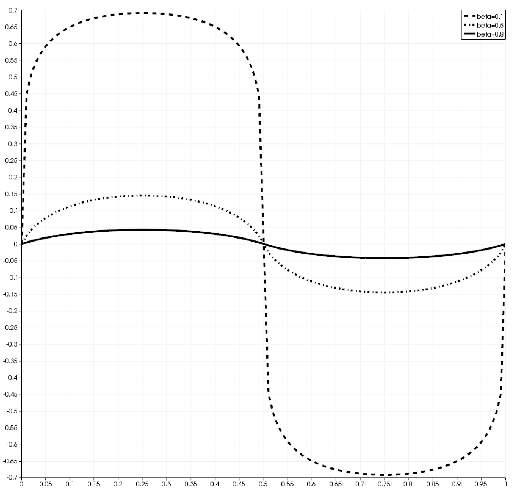
4.1. Numerical Illustration

We consider the unit square Ω=(0,1)2⊂ℝ2\Omega=(0,1)^{2}\subset\mathbb{R}^{2} and study numerically the efficiency in the approximation of uu the solution of

(−Δ)β​u=f,inΩ,u=0on∂Ω(-\Delta)^{\beta}u=f,\quad\text{in}\quad\Omega,\qquad u=0\quad\text{on}\quad\partial\Omega

where f:Ω→ℝf:\Omega\rightarrow\mathbb{R} is given for all (x1,x2)∈Ω(x_{1},x_{2})\in\Omega by

(57) f⁡(x1,x2)={1if(x1−0.5)​(x2−0.5)>00otherwise.f(x_{1},x_{2})=\left\{\begin{array}[]{ll}1&\qquad\text{if}\quad(x_{1}-0.5)(x_{2}-0.5)>0\\ 0&\qquad\text{otherwise.}\end{array}\right.

Notice that f∈H˙1/2−ϵ​(Ω)f\in\dot{H}^{1/2-\epsilon}(\Omega) for all ϵ>0\epsilon>0 (but not ϵ=0\epsilon=0) and consequently Theorem 4.3 and Remark 4.1 predict an error decay proportional to

ln⁡(1/h)​h2​s,\ln(1/h)h^{2s},

with

s={1,ifβ>34,2​(β+14),otherwise.s=\left\{\begin{array}[]{ll}1,&\quad\text{if}\quad\beta>\frac{3}{4},\\ 2(\beta+\frac{1}{4}),&\quad\text{otherwise}.\end{array}\right.

The errors ‖u−uhN‖L2\|u-u^{N}_{h}\|_{L_{2}} are computed using the first 300 modes in xx and yy (90000 modes) of the Fourier representation of the exact solution and the number of quadrature points is taken large enough not to influence the space discretization error. Four meshes are used to compute three observed rate of convergence

OROCi:=ln(ei/ei+1)/ln(hi/hi+1),i=1,2,3,OROC_{i}:=\ln\left(e_{i}/e_{i+1}\right)/\ln\left(h_{i}/h_{i+1}\right),\quad i=1,2,3,

where eie_{i} are the L2L_{2} errors and hih_{i} the diameter of the quasi-uniform subdivision ii. The average of the three observed rate of convergence A​R​O​CAROC are reported in Table 4 and are comparable with the rate predicted by Theorem 4.3 (see, Remark 4.1).

β<34\beta<\frac{3}{4} β>34\beta>\frac{3}{4}
0.1 0.2 0.3 0.4 0.5 0.6 0.7 0.8 0.9
AROC 0.92 1.06 1.22 1.4 1.52 1.72 1.86 1.94 1.96
THM 0.7 0.9 1.1 1.3 1.5 1.7 1.9 2.0 2.0
Table 4. Average observed rate of convergence (AROC) for different values of β\beta compared with the rates predicted by Theorem 4.3 (THM) ignoring the log term.

Figure 1 depicts the decay of the error ‖u−uhN‖L2\|u-u^{N}_{h}\|_{L_{2}} for different values of β\beta.

Refer to caption

Figure 1. L2L_{2}-errors for different values of β\beta versus the approximate mesh size diameter used for the computations. The number of quadrature points is taken large enough not to influence the errors. The corresponding average observed rate of convergence are reported in Table 4.

The solution for β=0.1\beta=0.1, 0.50.5 and 0.80.8 are depicted in figure 2 together with a cut over the horizontal line {y=0.25}\{y=0.25\}.

Refer to caption Refer to caption
Figure 2. Values of (−Δ)−β​f(-\Delta)^{-\beta}f when ff is the checkerboard function (57) for β=0.5\beta=0.5 (top left), β=0.8\beta=0.8 (top right) and β=0.1\beta=0.1 (bottom left). The difference in shape and magnitude is highlighted in the bottom right plots which depicts the values of these function along the line {y=0.25}\{y=0.25\} (β=0.1\beta=0.1 dashed line, β=0.5\beta=0.5 doted line, β=0.8\beta=0.8 solid line).

Acknowledgment

This work was supported in part by award number KUS-C1-016-04 made by King Abdulla University of Science and Technology (KAUST). The first author was also supported in part by the National Science Foundation through Grant DMS-1254618 while the second was also supported in part by the National Science Foundation through Grant DMS-1216551. In addition, the authors would like to thank E. Otarola, R.H. Nochetto and A. Salgado for fruitful discussions on the subject.

References

  • [1] Constantin Bacuta, James H. Bramble, and Joseph E. Pasciak. New interpolation results and applications to finite element methods for elliptic boundary value problems. East-West J. Numer. Math., 3:179–198, 2001.
  • [2] Oleg G. Bakunin. Turbulence and diffusion. Springer Series in Synergetics. Springer-Verlag, Berlin, 2008. Scaling versus equations.
  • [3] V. Balakrishnan. Fractional powers of closed operators and the semi-groups generated by them. Pacific J. Math., 10:419–437, 1960.
  • [4] Peter W. Bates. On some nonlocal evolution equations arising in materials science. In Nonlinear dynamics and evolution equations, volume 48 of Fields Inst. Commun., pages 13–52. Amer. Math. Soc., Providence, RI, 2006.
  • [5] M. Sh. Birman and M. Z. Solomjak. Spectral theory of selfadjoint operators in Hilbert space. Mathematics and its Applications (Soviet Series). D. Reidel Publishing Co., Dordrecht, 1987. Translated from the 1980 Russian original by S. Khrushchëv and V. Peller.
  • [6] J.H. Bramble and X. Zhang. The analysis of multigrid methods. In Handbook of numerical analysis, Vol. VII, Handb. Numer. Anal., VII, pages 173–415. North-Holland, Amsterdam, 2000.
  • [7] Luis Caffarelli and Luis Silvestre. An extension problem related to the fractional Laplacian. Comm. Partial Differential Equations, 32(7-9):1245–1260, 2007.
  • [8] P Carr, H Geman, DB Madan, and M Yor. The fine structure of asset returns: An empirical investigation. JOURNAL OF BUSINESS, 75(2):305–332, APR 2002.
  • [9] Peter Constantin and Jiahong Wu. Behavior of solutions of 2D quasi-geostrophic equations. SIAM J. Math. Anal., 30(5):937–948, 1999.
  • [10] M. Dauge. Elliptic Boundary Value Problems on Corner Domains. Lecture Notes in Mathematics, 1341, Springer-Verlag, 1988.
  • [11] G. Duvaut and J.-L. Lions. Inequalities in mechanics and physics. Springer-Verlag, Berlin, 1976. Translated from the French by C. W. John, Grundlehren der Mathematischen Wissenschaften, 219.
  • [12] A. Cemal Eringen. Nonlocal continuum field theories. Springer-Verlag, New York, 2002.
  • [13] Firoshi Fujita and Takashi Suzuki. Evolution Problems. Handbook of Numerical Analysis, II, Finite element methods. Part 1 (Ciarlet, P. G. and Lions, J.-L., eds.). North-Holland, Amsterdam, 1991.
  • [14] Ivan P. Gavrilyuk. An algorithmic representation of fractional powers of positive operators. Numer. Funct. Anal. Optim., 17(3-4):293–305, 1996.
  • [15] Ivan P. Gavrilyuk, Wolfgang Hackbusch, and Boris N. Khoromskij. H-matrix approximation for the operator exponential with applications. Numerische Mathematik, 92:83–111, 2002.
  • [16] Ivan P. Gavrilyuk, Wolfgang Hackbusch, and Boris N. Khoromskij. Data-sparse approximation to the operator-valued functions of elliptic operator. Math. Comp., 73(247):1297–1324, 2004.
  • [17] Ivan P. Gavrilyuk, Wolfgang Hackbusch, and Boris N. Khoromskij. Data-sparse approximation to a class of operator-valued functions. Math. Comp., 74(250):681–708, 2005.
  • [18] Ivan P. Gavrilyuk, Wolfgang Hackbusch, and Boris N. Khoromskij. Hierarchical tensor-product approximation to the inverse and related operators for high-dimensional elliptic problems. Computing, 74(2):131–157, 2005.
  • [19] Guy Gilboa and Stanley Osher. Nonlocal operators with applications to image processing. Multiscale Model. Simul., 7(3):1005–1028, 2008.
  • [20] J.-L. Guermond. The LBB condition in fractional Sobolev spaces and applications. IMA J. Numer. Anal., 29(3):790–805, 2009.
  • [21] M. Ilic, F. Liu, I. Turner, and V. Anh. Numerical approximation of a fractional-in-space diffusion equation. I. Fract. Calc. Appl. Anal., 8(3):323–341, 2005.
  • [22] M. Ilic, F. Liu, I. Turner, and V. Anh. Numerical approximation of a fractional-in-space diffusion equation. II. With nonhomogeneous boundary conditions. Fract. Calc. Appl. Anal., 9(4):333–349, 2006.
  • [23] R.B. Kellogg. Interpolation between subspaces of a hilbert space. Technical report, Univ. of Maryland,, Inst. Fluid Dynamics and App. Math., Tech. Note BN-719, 1971.
  • [24] John Lund and Kenneth L. Bowers. Sinc methods for quadrature and differential equations. Society for Industrial and Applied Mathematics (SIAM), Philadelphia, PA, 1992.
  • [25] B. M. McCay and M. N. L. Narasimhan. Theory of nonlocal electromagnetic fluids. Arch. Mech. (Arch. Mech. Stos.), 33(3):365–384, 1981.
  • [26] William McLean and Vidar Thomée. Iterative solution of shifted positive-definite linear systems arising in a numerical method for the heat equation based on Laplace transformation and quadrature. ANZIAM J., 53(2):134–155, 2011.
  • [27] Sergey Nazarov and Boris Plamenevsky. Elliptic problems in domains with piecewise smooth boundaries. De Gruyter expositions in mathematics, De Gruyter, 1994.
  • [28] R.H. Nochetto, E. Otarola, and A.J. Salgado. A PDE approach to fractional diffusion in general domains. part I: A priori error analysis. submitted.
  • [29] S. A. Silling. Reformulation of elasticity theory for discontinuities and long-range forces. J. Mech. Phys. Solids, 48(1):175–209, 2000.
  • [30] Vidar Thomée. Galerkin finite element methods for parabolic problems. Springer series in computational mathematics. Springer, New York, 1997.
  • [31] Qianqian Yang, Ian Turner, Fawang Liu, and Milos Ilić. Novel numerical methods for solving the time-space fractional diffusion equation in two dimensions. SIAM J. Sci. Comput., 33(3):1159–1180, 2011.
  • [32] Toshio Yoshida. Functional Analysis. Springer-Verlag, New York, 1995.