A theory of minimal updates in holography

In this appendix we describe the structure of causal cones in the MERA. The causal cone $\mathcal{C}(\mathcal{R})$ of a local region $\mathcal{R}$ is the part of the tensor network that contains the evolution of the region under successive coarse-graining transformations. Causal cones in MERA have a characteristic form, resulting from the peculiar structure of the tensor network, as we now examine.

We consider the specific MERA scheme analyzed in the main text, namely the modified binary MERA on a one-diemsnional lattice $\mathcal{L}$ [25]. Let $\mathcal{R}$ be a region of $l_{0}$ contiguous sites in $\mathcal{L}$, and let $l_{s}$ be the number of effective sites contained within the causal cone $\mathcal{C}(\mathcal{R})$ at depth $s$. In a single step of the coarse-graining transformation, the disentanglers $u$ act to spread the support of the causal cone by at most two sites, while the isometries $w$ act to compress the support by roughly a factor of two. If $l_{s}\gg 1$ sites are enclosed by the causal cone at depth $s$ then, under a layer of coarse graining, the action of the isometries dominates and the support of the causal cone shrinks by roughly a factor of two, i.e. $l_{s+1}\approx l_{s}/2$, see Fig. 5(a). We refer to this as the shrinking regime of the causal cone. Conversely, if $l_{s}=2$ then the spread of the support from the disentanglers is exactly balanced by the shrinking of the support from the isometries, and the causal cone remains at a fixed width, i.e. $l_{s+1}=l_{s}$. We refer to this as the stationary regime of the causal cone. Thus the causal cone $\mathcal{C}(\mathcal{R})$ of a region $\mathcal{R}\in\mathcal{L}$ of $l_{0}\gg 1$ sites is in the shrinking regime up to some crossover depth $s^{\textrm{c}}\approx\log_{2}(l_{0})$ after which it remains in the stationary regime, see Fig. 5(c).

In this appendix we review Wilson’s numerical renormalization group (NRG) [1, 2, 3, 24]. First we recount Wilson’s original arguments justifying the validity of the approach. Then we describe the technical details of its implementation.

NRG is a method for computing the low energy subspace of a one-dimensional lattice Hamiltonian of the form,

that we shall refer to as a Wilson chain Hamiltonian. The nearest neighbor term $\Lambda^{-s}h^{\mbox{\tiny W}}_{[s,s+1]}$ consists of a two site Hermitian operator $h^{\mbox{\tiny W}}_{[s,s+1]}$ that is independent of $s$ multiplied by the negative power of an amplitude $\Lambda>1$. Note that this is the form of the the effective Hamiltonian obtained, and subsequently solved, by Wilson in his solution to the Kondo impurity problem. For concreteness we shall henceforth set $\Lambda=10$ (although the following arguments remain valid for any $\Lambda>1$) and also assume that each site $s$ in $\mathcal{L}$ is associated to a two dimensional vector space $\mathbb{V}_{s}$, such that $h^{\mbox{\tiny W}}_{[s,s+1]}$ could be represented as a $4\times 4$ hermitian matrix. We further assume that the spacing of the eigenvalues of $h^{\mbox{\tiny W}}$ is of order unity.

It is possible to understand the qualitative features of the energy spectrum of a Wilson chain Hamiltonian just from the peculiar form the Hamiltonian takes (without the need to specify the local interactions $h^{\mbox{\tiny W}}$), as we now discuss. First we define, for $s\leq s_{\textrm{max}}$, the block Hamiltonian $H_{s}$ as the part of the original Hamiltonian $H^{\mbox{\tiny W}}$ that is supported on sites $[0,1,\cdots,s]$, with Hilbert space

and which consists of terms

Notice that the final block Hamiltonian in the series reproduces the full Wilson chain Hamiltonian, i.e. ${H_{{s_{\max}}}}=H^{\mbox{\tiny W}}$. Perturbation theory can be used to gain an understanding of the Wilson chain by treating the local couplings in $H^{\mbox{\tiny W}}$ with small prefactors (i.e. those at greater distance $s$ from the start of the chain) as perturbations of the local couplings with larger prefactors, as we now describe. By assumption the first block Hamiltonian, $H_{0}\equiv h_{[0]}$, has two energy levels that differ in magnitude by order unity. The spectrum of $H_{1}=H_{0}+\frac{1}{10}h_{[0,1]}$ can be understood by considering $\frac{1}{10}h_{[0,1]}$ as a perturbation of $H_{0}$; the two energy levels of $H_{0}$ are each split into two further levels that differ by $\sim\tfrac{1}{10}$. Likewise, we could then understand the spectrum of $H_{2}=H_{1}+\frac{1}{10^{2}}h_{[1,2]}$ by considering $\frac{1}{10}h_{[1,2]}$ as a perturbation of $H_{1}$ that splits each of its energy levels by $\sim\tfrac{1}{100}$ etc. Thus the spectrum of $H_{s}$ for any $s$, and, by extension the full Hamiltonian $H^{\mbox{\tiny W}}$, generically takes the form as shown Fig. 6(a). The numerical renormalization group (NRG) formalizes this perturbative understanding of Wilson chains into an algorithm for their solution.

Consider that we are interested in identifying a $\chi$ dimensional subspace $\mathbb{H}_{s_{\textrm{max}}}$ of the Hilbert space of $\mathcal{L}$ (where $\chi$ is some adjustable refinement parameter),

such that the Wilson chain $H^{\mbox{\tiny W}}$, when projected onto this subspace, is an effective Hamiltonian that retains the proper low energy physics of the original. The NRG algorithm allows one to identify such a subspace through a sequence of steps; initially a subspace of first two lattice sites is identified,

and then, sequentially for all $s\leq s_{\textrm{max}}$, subspaces of larger lattice regions are identified,

where each subspace ${\mathbb{H}_{s}}$ is restrained to be (at most) $\chi$-dimensional.

The NRG algorithm prescribes that each subspace ${\mathbb{H}_{s}}$ can be chosen through consideration of only the part of the Hamiltonian $H_{s}$ that is supported on this block, ignoring the Hamiltonian terms from outside the block. In the first step the subspace ${\mathbb{H}_{1}}\subseteq\mathbb{V}_{0}\otimes\mathbb{V}_{1}$ is chosen by diagonalizing the block Hamiltonian $H_{1}=h_{[0]}+\tfrac{1}{10}h_{[0,1]}^{\mbox{\tiny W}}$ and retaining the space spanned by its (at most) $\chi$ eigenvectors of lowest energy. Then an isometry $v_{1}$ is formed from these eigenvectors which serves as a mapping to the reduced Hilbert space,

We now use isometry $v_{1}$ to obtain an effective block Hamiltonian $H_{2}^{\textrm{eff}}=v_{1}^{\dagger}H_{2}v_{1}$ for the initial block Hamiltonian $H_{2}$ of the first three lattice sites. Notice that, whereas the initial block Hamiltonian $H_{2}$ is defined on the Hilbert space ${\mathbb{V}_{0}}\otimes{\mathbb{V}_{1}}\otimes{\mathbb{V}_{2}}$, the effective Hamiltonian $H_{2}^{\textrm{eff}}$ is defined on the subspace ${\mathbb{H}_{1}}\otimes{\mathbb{V}_{2}}$.

This process is then iterated over larger blocks; one would next identify the subspace ${\mathbb{H}_{2}}\subseteq\mathbb{H}_{1}\otimes\mathbb{V}_{2}$ by forming an isometry $v_{2}$ from the span of the $\chi$ lowest energy eigenvectors of $H_{2}^{\textrm{eff}}$,

The isometry $v_{2}$ can then be used to generate an effective block Hamiltonian $H_{3}^{\textrm{eff}}=v_{2}^{\dagger}v_{1}^{\dagger}H_{3}v_{1}v_{2}$ from the original block Hamiltonian $H_{3}$, see Fig. 7(a). Alternatively, the effective block Hamiltonian $H_{3}^{\textrm{eff}}$ can be obtained from the previous block Hamiltonian $H_{2}^{\textrm{eff}}$ as,

see also Fig. 7(b).

Likewise in subsequent steps, for all $s\leq s_{\textrm{max}}$, each effective Hamiltonian $H^{\textrm{eff}}_{s}$ (which equates to the block Hamiltonian $H_{s}$ projected onto the subspace ${\mathbb{H}_{s-1}}\otimes{\mathbb{V}_{s}}$) is diagonalized and an isometry $v_{s}$ is formed from its $\chi$ eigenvectors of lowest energy. The isometry projects to the subspace ${\mathbb{H}_{s}}$,

and is used to generate next effective Hamiltonian $H^{\textrm{eff}}_{s+1}$ as,

see again Fig. 7(b), where $\mathbb{I}_{s-1}$ and $\mathbb{I}_{s+1}$ here denote the identity on Hilbert spaces ${\mathbb{H}_{s-1}}$ and ${\mathbb{V}_{s+1}}$ respectively. Thus the NRG algorithm generates a sequence of isometric tensors $v_{s}$ each, in general, mapping from a Hilbert space of dimension $2\chi$ to one of dimension $\chi$, whose product identifies the low energy subspace ${\mathbb{H}_{{s_{\max}}}}$ of the Wilson chain,

Notice that this sequence of isometries $v_{s}$ form a matrix product state (MPS) of bond dimension $\chi$, see Fig. 7(c).

A key aspect of the NRG algorithm is that the low energy subspace ${\mathbb{H}_{s}}$ of the block of the first $s$ lattice sites is chosen only through consideration of the part of the Hamiltonian $H_{s}$ that is supported on this block (while ignoring the Hamiltonian terms outside of the block). As discussed in the main text, this leads to a notion of directed influence in Wilson chains, which justifies the proposal of minimal updates.

The validity of the NRG algorithm is justified from perturbation theory: in identifying the low energy subspace of a block (consisting of the first $s$ sites of the Wilson chain of Eq. 6) only the part of the Hamiltonian within the block need be considered as all couplings that are outside of the block are weaker a factor of $\Lambda^{-1}$ (where it was assumed $\Lambda>1$). In the limit that the perturbation parameter $\Lambda$ approaches unity the method becomes less effective, and typically a subspace $\mathbb{H}_{s}$ of large local dimension $\chi$ must be retained in order to maintain accuracy. In his solution to the Kondo impurity problem [1, 2, 3], where the energy scale parameter of the Wilson chain was $\Lambda=\sqrt{2}$, Wilson retained $\chi>1000$ states in each effective Hamiltonian in order to achieve an accuracy of a few percent. In contemporary applications of NRG [24] it is computationally feasible to take $\chi$ at least an order of magnitude larger. If one has $\Lambda=1$ exactly, such that all local couplings are of the same magnitude (as in the case of a homogeneous chain), then the NRG approach is no longer justified and would likely fail [35].

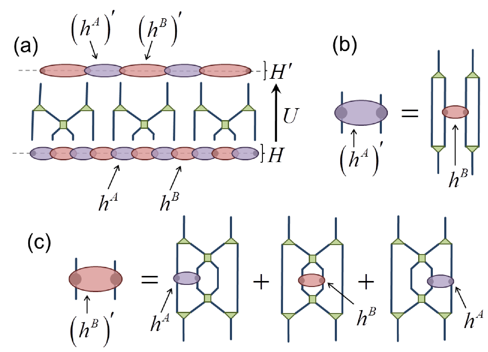
The scale invariant MERA offers a natural representation of the (scale-invariant) ground state of a gapless Hamiltonian at a critical point. Here we discuss the manifestation of scale-invariance in a specific MERA scheme, namely the modified binary MERA for one-dimensional systems (as introduced in Ref.28), which is the one employed in this paper, see Fig. 1(a). This scheme differs from previous implementations of the scale-invariant MERA [29, 27] in several details. Most significantly, the coarse-graining scheme that the modified binary MERA arises from yields effective Hamiltonians that are translation invariant under shifts of two sites (even if the initial Hamiltonian was invariant under shifts of a single site), whereas previously considered schemes [29, 27] yield effective Hamiltonians that are invariant under single site shifts. Consider a local $1D$ Hamiltonian $H$ of the form,

with $h^{A}$ and $h^{B}$ two potentially different nearest-neighbor couplings, and index $r$ labeling position on the lattice $\mathcal{L}$. Under coarse-graining with a single layer $U$ of the modified binary MERA, see Fig. 8(a), the Hamiltonian $H$ is mapped to a new Hamiltonian, $H\stackrel{{\scriptstyle U}}{{\longrightarrow}}H^{\prime}$, on a coarser lattice $\mathcal{L}^{\prime}$, where the new Hamiltonian $H^{\prime}$ is of the form,

for some new local couplings $\left({h^{A}}\right)^{\prime}$ and $\left({h^{B}}\right)^{\prime}$, and where index $r$ now labels position on $\mathcal{L}^{\prime}$. The new coupling $\left({h^{A}}\right)^{\prime}$ can be obtained through use of the (disconnected) ascending superoperator $\mathcal{A}_{D}$ on $h^{B}$,

see Fig. 8(b), while the new coupling $\left({h^{B}}\right)^{\prime}$ is obtained through use of (left, center, right) ascending superoperators $\mathcal{A}_{L}$ $\mathcal{A}_{C}$ and $\mathcal{A}_{R}$,

see Fig. 8(c). If the Hamiltonian $H$ is scale invariant fixed point of the MERA, and has had its energy spectrum shifted such that the ground state has zero energy, i.e. such that $\left\langle{{h^{A}}}\right\rangle=\left\langle{{h^{B}}}\right\rangle=0$, then the couplings transform self-similarly under coarse-graining,

i.e. such that $H^{\prime}=H/\Lambda$, where $\Lambda=2^{z}$ with $z$ is the dynamic critical exponent of $H$ (i.e. $z=1$ for a Lorentz invariant quantum critical point).

In the main text of this manuscript, it was asserted that the effective Hamiltonian $H_{\mathcal{R}}^{\mbox{\tiny W}}$ on the Wilson chain $\mathcal{L}^{\mbox{\tiny W}}_{\mathcal{R}}$, corresponding to the causal cone $\mathcal{C}(\mathcal{R})$ of a local region $\mathcal{R}$ generically takes the form described in Eq. 1 when the MERA describes a critical, scale-invariant state. Eq. 1 is the same form as the effective one-dimensional Hamiltonian that Wilson obtained in his solution to the (three-dimensional) Kondo impurity problem. Here we derive Eq. 1 explicitly by coarse-graining a one-dimensional Hamiltonian $H$ that is a scale-invariant fixed point of the MERA (in the modified binary scheme), and then outline how this derivation generalizes to systems in higher dimensions, see also Refs. 22, 32 for complimentary derivations of the effective Hamiltonian for the Wilson chain.

For a modified binary MERA defined on a $1D$ lattice $\mathcal{L}$, we consider the Wilson chain $\mathcal{L}^{\mbox{\tiny W}}_{\mathcal{R}}$ associated to the two-site region $\mathcal{R}\in\mathcal{L}$ as shown in Fig. 9(a). Let $\chi$ denote the dimension of each index connecting tensors in the MERA. Then the Wilson chain is a semi-infinite chain where each site has a vector space of dimension $\chi^{2}$, as two $\chi$-dimensional indices cross the surface of the causal cone between any depths $[s,s+1]$ in the MERA. The tensors in the MERA that are outside of the causal cone $\mathcal{C}(\mathcal{R})$ implement a coarse-graining transformation $U^{\mbox{\tiny W}}$ that maps the initial Hamiltonian $H$ into the effective Hamiltonian $H^{\mbox{\tiny W}}_{\mathcal{R}}$ on the Wilson chain, see Fig. 9(b). The effective Hamiltonian $H^{\mbox{\tiny W}}_{\mathcal{R}}$ can be written as,

for some nearest-neighbor coupling $\tilde{h}(s)$ that depends explicitly on position $s$. We now examine how these local couplings $\tilde{h}(s)$ can be computed, and derive a relationship between couplings at different positions on the Wilson chain. For simplicity we shall consider only the contribution to the effective Hamiltonian $H^{\mbox{\tiny W}}_{\mathcal{R}}$ that comes from the half of $H$ that is to the right of the region $\mathcal{R}$ (noting the left half yields an identical contribution). Let us begin by rewriting the right half of $H$ as,

where $K_{s}$ denotes the sum of all terms in $H$ supported on the lattice $\mathcal{L}$ in the interval of sites of distance between $\left[{r_{s}},{r_{s+1}}\right]$ to the right of $\mathcal{R}$, with $r_{s}$ defined as

For instance, $K_{1}$ is the sum of terms in the interval of sites at distance $\left[{r_{1}},{r_{2}}\right]=[1,2]$ from $\mathcal{R}$, which is just a single term,

while $K_{2}$ and $K_{3}$ are the sum of terms in the intervals of $\left[{r_{2}},{r_{3}}\right]=[2,5]$ and $\left[{r_{3}},{r_{4}}\right]=[5,10]$ respectively,

and so forth, see also Fig. 9(b). Let $\mathcal{A}_{s}$ denote the ascending superoperator that implements coarse-graining of the Hamiltonian term $K_{s}$ through one layer of the MERA (the explicit forms of $\mathcal{A}_{4}$, $\mathcal{A}_{3}$, $\mathcal{A}_{2}$ and $\mathcal{A}_{1}$ are depicted in Fig. 9(d-g)). Then the local coupling $\tilde{h}_{[s,s+1]}(s)$ of the effective Hamiltonian is obtained by coarse-graining $K_{s+1}$ a total of $s+1$ times,

In Fig. 9(c) we depict the coarse-graining of the term $K_{4}$, a particular case of Eq. 28, which is written as,

If the local Hamiltonian $H$ is invariant under coarse-graining with the MERA, as discussed in the previous section (see, in particular, Eq. 22), then it can be seen that the $K$ terms transform in a precise way under coarse-graining,

for all $s\geq 1$. Here $z$ is the dynamic critical exponent of $H$. If we define $h^{\mbox{\tiny W}}\equiv\mathcal{A}_{1}\left(K_{1}\right)$ then all local couplings $\tilde{h}_{[s,s+1]}(s)$ of the effective Hamiltonian $H^{\mbox{\tiny W}}_{\mathcal{R}}$, as written in Eq. 23, are all proportionate to this $h^{\mbox{\tiny W}}$,

Thus the effective Hamiltonian $H^{\mbox{\tiny W}}_{\mathcal{R}}$ for the Wilson chain is consistent with that proposed in Eq. 1, with the geometric decay of coupling strength $\Lambda=2^{z}$.

The essential features of the above derivation, which are geometric in nature, hold for MERA defined on higher dimensional lattices such that they also yield effective Hamiltonians of the form of Eq. 1 on their corresponding Wilson chains, as we now outline. Let us assume that we have a $d$-dimensional hypercubic lattice $\mathcal{L}$ on which a local Hamiltonian $H=\sum h$ and a scale invariant MERA are defined, and that we would like to understand the effective Hamiltonian $H^{\mbox{\tiny W}}_{\mathcal{R}}$ for the Wilson chain ${\mathcal{L}}^{\mbox{\tiny W}}_{\mathcal{R}}$ associated to a local region $\mathcal{R}$.

Given a local region $\mathcal{S}$ in $\mathcal{L}$ that is displaced by vector $\vec{r}$ from $\mathcal{R}$, the causal cones of the two regions will intersect roughly at depth $\sim\log_{2}\left|\vec{r}\right|$ (note that we are assuming that each layer of the MERA rescales the lattice by a factor $\tfrac{1}{2}$ in all spatial dimensions, as with the modified binary MERA), see Fig. 10(a-b). The depth at which the causal cones intersect informs us the scale at which an operator $o_{\mathcal{S}}$ that is supported on $\mathcal{S}$ is coarse-grained onto the Wilson chain ${\mathcal{L}}^{\mbox{\tiny W}}_{\mathcal{R}}$ associated to region $\mathcal{R}$. Thus one can partition the lattice $\mathcal{L}$ into a series of concentric (hypercubic) shells $\mathcal{R}_{s}$ about the local region $\mathcal{R}_{0}\equiv\mathcal{R}$, where shell $\mathcal{R}_{s}$ is roughly comprised of all sites at a distance between $2^{s-1}$ and $2^{s}$ sites away from $\mathcal{R}_{0}$, such that any operator that is supported on the shell $\mathcal{R}_{s}$ will be coarse-grained to a new local operator supported on sites $[s-1,s]$ of the Wilson chain ${\mathcal{L}}^{\mbox{\tiny W}}_{\mathcal{R}}$. Let us, as with Eq. 24 for the $1D$ MERA, rewrite the initial Hamiltonian as $H=\sum\nolimits_{s=0}^{\infty}K_{s}$ where each $K_{s}$ corresponds to the sum of all the couplings supported on the shell $\mathcal{R}_{s}$, see Fig. 10(c). It is then seen that the coupling $\tilde{h}_{[s,s+1]}(s)$ in the effective Hamiltonian for the Wilson chain arises through $s+1$ coarse-grainings of each $K_{s+1}$, i.e.

where each $\mathcal{A}_{s}$ represents the appropriate ascending superoperator that coarse-grains $K_{s}$ through one layer of the MERA, see Fig. 10(d). Roughly speaking, the term $K_{s+1}$ collects together $O(2^{d(s+1)})$ nearest neighbor terms in $H$, each of which has is then coarse-grained $(s+1)$ times to give the effective coupling of the Wilson chain $\tilde{h}_{[s,s+1]}(s)$. In a critical system in $d$ space dimensions the scaling dimension of a single Hamiltonian term is $\Delta=d+z$, where $z$ is the dynamic critical exponent of $H$, with $z=1$ for Lorentz invariant quantum critical points. This implies that one such term is reduced by a factor $2^{-\Delta}=2^{-(d+z)}$ with each coarse-graining step. Hence the effective couplings are of the form,

where the independence of $h^{\mbox{\tiny W}}_{[s,s+1]}$ on $s$ follows from the invariance of $H$ both under translations and re-scaling transformations, the amplitude $\Lambda^{-s}$ results from,

Notice that Eq. 33 is the same as Eq. 31, which was derived explicitly for a one-dimensional system.

In the main text we have discussed a theory of minimal updates in the holographic description of a many-body ground state. For simplicity, we have considered a translation invariant system that is gapless fixed-point of the RG flow, and therefore invariant under changes of scale (as implemented by means of discrete coarse-graining transformations). However, the essential parts of our arguments do not rely on translation or scale invariance, and the proposed minimal updates also apply in the absence of such space symmetries.

In this appendix we address the case of a gapped system in a topologically trivial phase, where the ground state can be described by a finitely correlated MERA [29]. A finitely correlated MERA has a set number of layers $s_{\textrm{max}}$, see Fig. 11(a), and is expected to offer a good approximation to the ground state of a gapped Hamiltonians $H$ (in a topologically trivial phase) when the correlation length $\xi$ fulfills $\xi<2^{s_{\textrm{max}}}$.

The justification for directed influence in finitely correlated MERA and its consequence in permitting a minimal update of the MERA under a local change to the Hamiltonian is analogous to the case analyzed in the main text. However, some implications of directed influence are different. One difference is that modifying a finitely correlated MERA within a causal cone $\mathcal{C}(\mathcal{R})$ only affects the ground state properties within some localized region around $\mathcal{R}$. Consider, for instance, taking the expected value of a local observable $o$ from two different finitely correlated MERA $\big|\psi\big\rangle$ and $\big|\tilde{\psi}\big\rangle$, each with a fixed number $s_{\textrm{max}}$ layers, whose tensors only differ within the causal cone $\mathcal{C}(\mathcal{R})$ of a local region $\mathcal{R}\in\mathcal{L}$. Here, one can identify a larger region $\mathcal{S}\in\mathcal{L}$, which is defined as the set of all sites whose causal cone intersects with $\mathcal{C}(\mathcal{R})$ (notice that this roughly corresponds to the shell of thickness $\sim 2^{s_{\textrm{max}}}$ about $\mathcal{R}$, see Fig. 11(c)), such that the expectation value of any local observable is identical between the two MERA whenever the observable is outside the support of $\mathcal{S}$, i.e.

for all local observables $o$. Recall that, in the case of scale invariant MERA, changing the tensors within a causal cone can affect the expectation value of a local observable everywhere on the lattice $\mathcal{L}$. This difference arises as it is only in finitely correlated MERA that separated regions of the lattice can be causally disconnected, i.e. such that there is no overlap in the respective causal cones of the regions.

Another difference in dealing with a finitely correlated MERA is that their corresponding Wilson chains are finite $1D$ lattices of $(s_{\textrm{max}}+1)$ sites, see Fig. 11(d)), as opposed to the semi-infinite $1D$ lattices that arise from scale invariant MERA. Let us examine, given a local Hamiltonian $H$ defined on the lattice $\mathcal{L}$, the computation of the effective Hamiltonian $H^{\mbox{\tiny W}}_{\mathcal{R}}$ corresponding to a local region $\mathcal{R}\in\mathcal{L}$. It can be seen that only part of the local Hamiltonian $H$ near the region $\mathcal{R}$ contributes to the effective Hamiltonian; specifically, if we once more partition the local Hamiltonian into terms $K_{s}$ supported on a series of concentric shells, as described by Eqs. 24 and 25, then it is only terms $K_{s}$ for $s\leq s_{\textrm{max}}$ that are coarse-grained into couplings on the effective Hamiltonian $H^{\mbox{\tiny W}}_{\mathcal{R}}$ (whereas terms $K_{s}$ for $s>s_{\textrm{max}}$ only shift the overall energy levels of $H^{\mbox{\tiny W}}_{\mathcal{R}}$ by an irrelevant constant, see Fig. 11(e)).

References

- [1] K.G. Wilson, Adv. Math., Volume 16, Issue 2, Pages 170-186 (1975).
- [2] K.G. Wilson, Rev. Mod. Phys. 47, 773 (1975).
- [3] M.E. Fischer, Rev. Mod. Phys. 70, 653 (1998).
- [4] J. Maldacena, Adv. Theor. Math. Phys. 2, 231 (1998).
- [5] E. Witten, Adv. Theor. Math. Phys. 2, 253 (1998).
- [6] R. Bousso, Rev. Mod. Phys. 74, 825 (2002).
- [7] G. Vidal, Phys. Rev. Lett. 99, 220405 (2007).
- [8] For an introduction, see G. Vidal, ”Entanglement Renormalization: an introduction”, chapter 5 in the book ”Understanding Quantum Phase Transitions”, edited by Lincoln D. Carr (Taylor Francis, Boca Raton, 2010).
- [9] G. Vidal, Phys. Rev. Lett., 101, 110501 (2008).
- [10] By holographic description we mean one that extends in an additional dimension corresponding to scale or RG flow. The MERA is then a holographic description in this general sense. The term ’holography’ may also be used in a more restricted sense, where one expects the scale dimension to be locally equivalent to the other space dimensions in the bulk. By studying properties of the MERA, we expect to learn about the general structure of RG-based holographic descriptions. Examples of those are modularity [22], and the mapping of a global symmetry at the boundary into a local symmetry in the bulk [21].
- [11] B. Swingle, Phys. Rev. D 86, 065007 (2012).
- [12] G. Evenbly, G. Vidal, Phys. Rev. Lett. 112, 220502 (2014).
- [13] G. Evenbly, G. Vidal, Phys. Rev. Lett. 112, 240502 (2014).
- [14] B. Swingle, pre-print arXiv:1209.3304.
- [15] M. Nozaki, S. Ryu, and T. Takayanagi, JHEP 10, 193 (2012).
- [16] G. Evenbly, G. Vidal, J. Stat. Phys. 145, 891 (2011).
- [17] J. Molina-Vilaplana and P. Sodano, JHEP 10, 11 (2011).
- [18] C. Beny, New J. Phys. 15 (2013) 023020.
- [19] H. Matsueda, M. Ishihara, and Y. Hashizume, Phys. Rev. D 87, 066002 (2013).
- [20] T. Hartman, J. Maldacena, JHEP 5, 14 (2013).
- [21] S. Singh, G. Vidal, Phys. Rev. B 88, 121108(R) (2013).
- [22] G. Evenbly, G. Vidal, J. Stat. Phys. 157, 931 (2014).
- [23] In the Hamiltonian formalism, a -dimensional lattice describes a system in space-time dimensions. Thus, a critical ground state in space dimensions and its MERA representation in dimensions (in both cases, there is no time dimension, given that the time evolution of a ground state is trivial), should be thought of as analogous to a CFT in dimensions and AdS in dimensions, respectively.
- [24] R. Bulla, T. Costi, and T. Pruschke, Rev. Mod. Phys. 80, 395 (2008).
- [25] There are many possible MERA schemes even in just dimensions, depending on aspects such as how many sites are coarse-grained into a single site, or where the disentanglers are placed, see Ref. 28.
- [26] V. Giovannetti, S. Montangero, R. Fazio, Phys. Rev. Lett. 101, 180503 (2008).
- [27] R.N.C. Pfeifer, G. Evenbly, and G. Vidal, Phys. Rev. A 79, 040301(R) (2009).
- [28] G. Evenbly and G. Vidal, ”Quantum Criticality with the Multi-scale Entanglement Renormalization Ansatz”, chapter 4 in the book ”Strongly Correlated Systems. Numerical Methods”, edited by A. Avella and F. Mancini (Springer Series in Solid-State Sciences, Vol. 176 2013), arXiv:1109.5334.
- [29] G. Evenbly and G. Vidal, Phys. Rev. B 79, 144108 (2009).
- [30] The minimal updates discussed in this paper are not restricted to a small region . For instance, in boundary or interface problems, region can correspond to a semi-infinite line, plane, etc [22].
- [31] M. Oshikawa and I. Affleck, Nucl. Phys. B 495:533-582 (1997).
- [32] G. Evenbly, R. N. C. Pfeifer, V. Pico, S. Iblisdir, L. Tagliacozzo, I. P. McCulloch, G. Vidal, Phys. Rev. B 82, 161107(R) (2010).
- [33] M. Fannes, B. Nachtergaele, and R. F. Werner, Commun. Math. Phys. 144, 443 (1992).
- [34] S. Ostlund and S. Rommer, Phys. Rev. Lett. 75, 3537 (1995).
- [35] S.R. White, Phys. Rev. Lett. 69, 2863 (1992).
- [36] If the update were not restricted to the causal cone then a variational algorithm based upon optimally preserving the support of the ground state’s reduced density matrix [35] would likely yield location-dependent tensors , given that the reduced density matrix of a region depends on the distance between and the location of the impurity. Thus the Hamiltonian will be coarse-grained into an effective Hamiltonian made of location-dependent terms: the initially localized impurity has effectively become delocalized. That the location-independent bulk tensors already do a good (though perhaps not optimal) job of preserving the support for all away from the impurity is a key result of minimal updates.
Appendix A Causal cones in the MERA