Generalized Alpha Investing: Definitions, Optimality Results, and Application to Public Databases
Abstract
The increasing prevalence and utility of large, public databases necessitates the development of appropriate methods for controlling false discovery. Motivated by this challenge, we discuss the generic problem of testing a possibly infinite stream of null hypotheses. In this context, Foster and Stine (2008) suggested a novel method named Alpha Investing for controlling a false discovery measure known as mFDR. We develop a more general procedure for controlling mFDR, of which Alpha Investing is a special case. We show that in common, practical situations, the general procedure can be optimized to produce an expected reward optimal (ERO) version, which is more powerful than Alpha Investing.
We then present the concept of quality preserving databases (QPD), originally introduced in Aharoni et al. (2011), which formalizes efficient public database management to simultaneously save costs and control false discovery. We show how one variant of generalized alpha investing can be used to control mFDR in a QPD and lead to significant reduction in costs compared to naïve approaches for controlling the Family-Wise Error Rate implemented in Aharoni et al. (2011).
1 Introduction
As the extent of available data and scientific questions being addressed through hypothesis testing continues to increase, statisticians are required to develop appropriate approaches that control false discoveries in large scale testing to assure statistical validity of discoveries and publications, while facilitating efficient use of the data and assuring maximal power to the studies. For example, modern genome-wide association studies already perform on the order of one million tests per study. Issues of power, sample size and false discoveries in such studies are recognized as a major concern [7].
This situation has given rise to a vast and growing literature on multiple comparison control and corrections, encompassing a variety of methods for controlling a range of measures of false discovery. Let denote the number of rejected null hypotheses (discoveries), and the number of rejected null hypotheses which are true nulls (false discoveries). The two most commonly used measures of false discovery are the Family-Wise Error Rate (FWER) and False Discovery Rate (FDR), defined as follows.
FWER is the probability of making one or more false discoveries, while FDR is the expected percentage of false discoveries among the total number of discoveries.
Given a measure of false discovery, one needs to develop statistical testing approaches that guarantee control over this measure. The simplest approaches typically assume nothing about the statistical hypothesis testing setup and guarantee control in all possible scenarios. Such is the Bonferroni correction for controlling FWER. The FDR control procedure developed by [3] assumes the test statistics are independent or that they have a positive regression dependency [4]. A modified, more conservative version of this procedure covers all other forms of dependency [4].
An interesting situation arises when hypotheses arrive sequentially in a stream, and the testing procedure should determine whether to accept or reject each of them without waiting for the end of stream. Organizing hypotheses sequentially may be a choice based on scientific considerations [5], but it may also be an external constraint, whereby the testing of each hypothesis is performed as it arrives and a conclusion is taken.
Such a constraint occurs when attempting to apply procedures for controlling false discovery on a public database. Such databases, accessed or distributed through the Internet, are used by research groups worldwide, and are becoming increasingly pervasive. Examples include Stanford university’s HIVdb [12] which serves the community of anti-HIV treatment researches, WTCCC’s large-scale data for whole-genome association studies [17] which is distributed to selected research groups, and the NIH Influenza virus resource [2], often used to identify complex dependencies in the virus genome. Some databases are targeted for a specific type of hypotheses and contain built-in facilities for executing tests, e.g., ProMateus [11], a collaborative web server for automatic feature selection for protein binding-sites prediction.
The need to control false discovery across multiple research groups without sacrificing too much power is repeatedly acknowledged [13, 15, 16, 8]. Since such a public database serves multiple researchers, working independently at different times, a procedure for controlling false discovery in this context must be sequential, without prior knowledge of even the number of hypotheses that is going to be tested. Such a framework, termed ”Quality Preserving Database” (QPD), is discussed in [1]. A QPD controls false discovery by prescribing the levels of the tests performed by its users. To avoid power loss over time, the database size is continually augmented, and the costs of obtaining additional data are fairly distributed among database users based on their activity. Thus a QPD is potentially handling an infinite series of tests.
The QPD implementation described in [1] uses a sequential testing procedure known as Alpha Spending [5], which is closely related to Bonferroni correction. Alpha Spending uses an -wealth function that contains a pool of available level for testing. If the ’th test is conducted at level , then this amount is subtracted from the pool, . Initializing and requiring , guarantees that , and hence that is controlled at level .
In the search for a sequential procedure for controlling , a modified measure has been employed, [5]:
| (4) |
where is some constant, typically chosen to be . A sequential procedure known as Alpha Investing [5] controls at level . Alpha Investing is similar to Alpha Spending in its usage of an -wealth function , except in Alpha Investing this function not only decreases, but sometimes increases. Whenever a hypothesis is rejected, a reward is added to , allowing higher levels and higher power for subsequent tests.
In this paper we define a more general framework we term Generalized Alpha Investing. This framework allows more control over the level of the ’th test and the reward obtained if the hypothesis is rejected. We show that there is a trade-off between the two, i.e., if a higher level is chosen for the ’th test, then the reward decreases, and vice versa. Therefore, our general framework changes the meaning of the wealth function. Instead of just -wealth, becomes an abstract potential function, and the amounts withdrawn from it can be converted to various combinations of level and reward, of which Alpha Investing and Alpha Spending are special cases.
We define an optimality criterion which determines what is the optimal usage of amounts withdrawn from , and show that reaching the optimum is feasible in the case of uniformly most powerful tests with continuous distribution functions, a single parameter, and a simple null hypothesis. We demonstrate in simulations that this optimized variant is significantly more powerful than Alpha Investing for a range of realistic scenarios.
We also present another special case of Generalized Alpha Investing which is more easily combined with systems that rely on Alpha Spending. We term this last variant Alpha Spending with Rewards. We demonstrate how Alpha Spending with Rewards can replace Alpha Spending in a QPD implementation. This replaces with as the controlled measure, in exchange for reduced usage costs. Note that Alpha Investing, as formulated in [5], cannot be combined with a QPD, while Alpha Spending with Rewards smoothly integrates with it. Thus our new implementation demonstrates both the advantage of a QPD, as well as the advantages of our Generalized Alpha Investing approach.
The rest of the paper is organized as follows. Section 2 provides a concise summary of the Alpha Investing procedure and mFDR as described in [5]. Section 3 describes our generalization of the Alpha Investing procedure, its special cases and associated optimality results. Section 4 formally defines the QPD along the lines of [1] and demonstrates how it can be combined with Alpha Spending with Rewards, to control and achieve the QPD goals while imposing lower costs on users.
2 Alpha Investing and mFDR
2.1 Notation and Assumptions
Following a notation similar to [5], we consider the problem of testing null hypotheses, , ,…,. A random variable indicates whether was rejected, and counts the total number of rejections. Similarly, indicates the case is true and is rejected (i.e., type-I error), and tracks total number of type-I errors.
Let be the parameter space assumed by the ’th test. The null hypothesis is defined as a subset , and the alternative hypothesis is . is the true parameter value, thus is true if . We denote by and the combined parameter space and true parameter values of all tests, respectively. We use the notation and to denote probability distribution and expectation when assuming . We denote the level of the ’th test by .
In our analysis we require an additional, uncommon measure we term “Best Power”. Denoted by , we define it as the maximal probability of rejection for any parameter value in the alternative hypothesis. The following definition formalizes it.
Definition 2.1
The Best Power, , of testing a null hypothesis is
| (5) |
In Best Power we measure the upper bound on the power, which is often 1. The simplest case in which , is when the alternative hypothesis is simple, e.g., in Neyman-Pearson type tests. In this case the best power is simply the power computed for the alternative hypothesis. Another case in which is when the alternative hypothesis is limited to a finite range. For example, a situation where a z-test is performed to test the effect of a drug on some clinical measure (we assume the standard deviation of this measure is known from previous studies). Since clinical measures are confined to some finite, biologically plausible range, it follows that the alternative hypothesis must be limited in range.
Similarly to [5], the results in this paper require the following assumption on the dependence between the tests in the sequence.
Assumption 2.2
| (6) | |||
| (7) |
Assumption 2.2 requires that the level and power traits of a test hold even given the history of rejections. This is somewhat weaker than requiring independence.
2.2 Alpha Spending
An Alpha Spending procedure is a simple procedure for multiple hypothesis testing. It maintains a pool of nonnegative -wealth , where is the initial pool and is the remaining wealth after the ’th test. The level allocated for the ’th test, , is subtracted from the wealth, i.e., .
Since the wealth must remain non negative, this procedure enforces the invariant . Hence this procedure guarantees a bound of on the Family-Wise Error Rate (FWER), the probability of falsely rejecting any null hypothesis, .
The major drawback of this and other Bonferroni based procedures is that the FWER measure is often too conservative, hence aiming to control it results in loss of power. In the following we discuss less conservative measures and procedures for controlling them.
2.3 FDR and mFDR
In [3] the concept of False Discovery Rate is introduced, which may be defined as follows: . Since it is trivially true that , power gain is to be expected when aiming to control instead of . Furthermore, under the complete null hypothesis assumption, i.e., when assuming all null hypotheses are true, it holds that . Controlling under this assumption is referred to as controlling it in the weak sense.
Multiple variants of have been suggested in the literature, such as which drops the term [14], and various variants termed Marginal False Discovery Rate (mFDR), based on the form , with or without adding a constant to the denominator [3].
We adopt the form and notation of [5], in defining as follows.
| (8) |
Under the complete null hypothesis assumption, it is easy to show that implies . Since , then similar to the standard , controlling with set to implies control over in the weak sense.
In the rest of this paper we only refer to control in the strong sense, i.e., a procedure that controls at level will guarantee it is bounded by for any value of the unknown parameters .
2.4 Alpha Investing
Alpha Investing [5] is a procedure that controls at level for any given choice of and . It is defined as follows.
Similarly to Alpha Spending, the procedure uses a pool of -wealth, . While in Alpha Spending we only subtract amounts from this wealth until it is depleted, here we sometimes put back wealth to the pool, hence the increased power.
A deterministic function , known as the alpha investing rule, determines the level of the next test as a function of the current rejection history and the initial wealth.
| (9) |
The -wealth is initialized and updated as follows.
i.e., if is accepted, then the amount is subtracted from the wealth. If it is rejected, a reward is added.
The following definition summarizes the Alpha Investing Procedure
Definition 2.3
3 Generalized Alpha Investing Procedure
3.1 Definition
We now present a more general definition of Alpha-Investing-like procedures. We show that the original Alpha Investing procedure is a special case of it, as well as Alpha Spending. We show further an additional special case which is better suited than Alpha Investing for performing Neyman-Pearson tests.
Our generalization starts with a generalized investing rule , which now separately determines three quantities: The level of the test, , the amount subtracted from the wealth, and the reward received upon rejection.
| (13) |
We no longer refer to as -wealth, since its relation to the level of the test is quite indirect. We refer to it more generally as a potential function. Its initialization and update rule are now:
Note one subtle point: In the original Alpha Investing (equation 2.4), the amount is subtracted from the wealth only if we fail to reject . Here the amount is subtracted unconditionally. This change is introduced to simplify the analysis below.
Definition 3.1
Before analyzing this framework, let us demonstrate that the original Alpha Investing procedure is a special case of it.
Proposition 3.2
Alpha Investing procedure is a special case of the Generalized Alpha Investing procedure.
In the generalized framework, let us choose and , where is some constant such that . Substituting in the update rule 3.1 we get , which is the Alpha Investing update rule. It only remains to show that the constraint 17 is satisfied. This holds since and .
We now proceed to show that the Generalized Alpha Investing Procedure indeed controls . We follow the same main ideas as the proof for alpha-investing in [5].
Theorem 3.3
Given Assumption 2.2, a Generalized Alpha Investing Procedure controls at level .
Requiring is equivalent to requiring: . Since the procedure uses a non-negative potential function , it is sufficient to require .
Let . Lemma 7.1 proves is a sub-martingale with respect to . From the sub-martingale properties it follows that . Since by definition and , we get . Hence .
3.2 The Generalized Alpha Investing Trade-off Function and Wealth Management
In the Alpha Spending procedure, whenever a test is performed at level , the same amount is subtracted from the -wealth, . In the Alpha Investing procedure, for a test at level we need to subtract a larger amount of , as prescribed by equation 2.4. Both procedures do not specify a particular way for managing the -wealth, but leave it to the user to define rule 9.
Generalized Alpha Investing procedure offers even more freedom. It requires the user to choose separately the level of the test , the amount subtracted from the potential function , and the reward . Any choice is valid as long as the potential function does not become negative, , and the reward satisfies constraint 17.
In order to study the relation between the three user defined parameters , , and , let us fix on a given amount, and set the reward to the maximal value allowed by constraint 17. According to this constraint, now becomes a function of (note that used in the constraint is also a function of ).

Figure 1 shows as a function of , for a test about the mean of a normal distribution with unknown variance. We used a -statistic with degrees of freedom, , , , and . The shape of the line reflects the two parts of constraints 17: and , where the convex part of the line left of the ’knee’ is the latter and the right part is the former. It shows the trade-off the Generalized Alpha Investing offers between the level of the test and the reward . At one extreme, setting the maximal possible level results in no reward, . At the other extreme, the reward tends to infinity, .
In the following subsections we explore various options of trade-off between and , as shown in figure 1. Note that we do not deal theoretically with the question of how to choose . As in Alpha Investing and Alpha Spending, management of the pool is left for user discretion. In the simulation results of Subsection 3.5 and Section 5 we empirically explore some natural candidates.
Alpha Investing is a special case of Generalized Alpha Investing, where . The corresponding point is marked by a circle in the figure. This seems like an arbitrary point, but Subsection 3.4 shows it is not.
Subsection 3.3 shows that the extreme point of , is in fact Alpha Spending. It further shows another special case we term Alpha Spending with Rewards which has some practical benefits. The rhombus marked in the figure is for the case , where is a configurable parameter of the Alpha Spending with Rewards method, as defined in the next subsection. Other values of may reach other points in the figure.
Subsection 3.4 shows that, under certain assumptions, the ’knee’ noticeable in the figure is the optimal point for a criterion we term Expected Reward Optimal (ERO). We call this special case ERO Alpha Investing.
3.3 Alpha Spending with Rewards
In Generalized Alpha Investing the level of the test may be chosen independently of choosing the amount subtracted from the potential function. A special case, therefore, is when choosing , for some constant . This special case is of interest, since it can be viewed as direct extension of Alpha Spending: By scaling the units of the potential function , we can restore its original meaning of -wealth, and have the level of the test be directly subtracted from it. This is in contrast to Alpha Investing, where is non-linearly dependent on . We term this special case “Alpha Spending with Rewards”, defined more formally next.
We define an Alpha Spending with Rewards rule, that determines the level of the ’th test and the reward in case is rejected, based on and the history of rejections.
| (18) |
The wealth is initialized and updated as follows.
Definition 3.4
We now proceed to show Alpha Spending with Rewards is indeed a special case of the Generalized Alpha Investing Procedure, hence it controls at level .
Proposition 3.5
Alpha Spending with Rewards is a special case of the Generalized Alpha Investing procedure.
Choosing , and we get a Generalized Alpha Investing procedure with potential function , costs and rewards .
Corollary 3.6
Given Assumption 2.2, Alpha Spending with Rewards controls at level .
Proposition 3.7
Alpha Spending is a special case of Alpha Spending with rewards, and hence of the Generalized Alpha Investing Procedure.
In an Alpha Spending with Rewards procedure, choosing , we get , and . Hence this is equivalent to Alpha Spending with initial wealth .
Choosing is the minimal value for that has nonnegative rewards. Increasing increases the rewards, at the expense of reducing .
Alpha Spending with Rewards can be more easily combined with systems based on Alpha Spending, since its equation for updating the -wealth is identical to that of Alpha Spending, except for the initialization and the rewards. This point is demonstrated in following sections with the QPD.
3.4 Optimizing the Generalized Alpha Investing Procedure
In this subsection we find the optimal point of trade-off between and , when given a potential investment amount .
Our criterion of optimality is , the expected reward of the current test. This is a natural optimization criterion, since aiming to increase our expected reward is related to the power of the current test as well as to our potential to perform additional tests. Note that as increases, increases but decreases because of constraint 17. Therefore it is not trivial to maximize their product, .
Since is an unknown parameter, we seek a procedure for which optimality is guaranteed for all , as in the following definition.
Definition 3.8
A Generalized Alpha Investing Procedure is expected reward optimal (ERO) if at any point in time , the procedure chooses and such that for any other values and and for any it holds that , where is the random variable corresponding to for a test executed at level .
An ERO procedure can be found under some assumptions on the relation between level and power. This occurs when choosing the and at the intersection between the two parts of constraint 17, as shown in figure 1. We term this choice ERO Alpha investing:
Definition 3.9
An ERO Alpha Investing procedure is a Generalized Alpha Investing procedure that chooses as the solution of and .
We now proceed to show that this is indeed an ERO procedure under certain assumptions. In the appendix we provide a general Theorem 7.2, which fully lists the set of required assumptions, and is rigorously proven. However, since these assumptions and proofs involve many technicalities, we provide here a simpler theorem, that captures some practical cases.
Theorem 3.10
For a series of uniformly most powerful tests with continuous distribution functions, a single parameter , and a simple null hypothesis , ERO Alpha Investing is an ERO procedure.
One simple case covered by Theorem 3.10 is a series of Neyman-Pearson tests, where both null and alternative hypotheses are simple. A more general case is when the tests are uniformly most powerful, and when the null hypothesis remains simple. Such a case may occur, for example, when performing a z-test with null hypothesis , and alternative (i.e., when it is known that is non-negative).
Now that we’ve established an ERO procedure exists, we proceed to show that for unbounded alternative hypothesis, this procedure in fact reduces to the original Alpha Investing.
Corollary 3.11
When the ERO Alpha Investing is an ERO procedure, the original Alpha Investing is also an ERO procedure if and only if .
Setting in Definition 3.9 yields , which is the level used by Alpha Investing for a given cost . Any other value of clearly yields different levels.
To summarize this subsection, we have shown that in some cases an ERO procedure can be found. In these cases, if the alternative hypothesis stretches to infinity, then the original Alpha Investing is identical to ERO Alpha Investing. However, if the alternative hypothesis is simple or limited in range, then ERO Alpha Investing will have larger expected rewards than Alpha Investing, and therefore we expect it to be more powerful.
The next subsection explores this expected theoretical gain in simulations.
3.5 Simulation Results
Procedure Tests True rejects False rejects mFDR Alpha Spending 10.000 0.283 0.041 0.032 Alpha Investing 15.908 0.435 0.064 0.044 Alpha Spending with Rewards (k=1) 15.188 0.416 0.061 0.043 Alpha Spending with Rewards (k=1.1) 17.888 0.476 0.066 0.044 ERO Alpha Investing 18.355 0.504 0.073 0.048
Procedure Tests True rejects False rejects mFDR Alpha Spending 66.000 0.559 0.043 0.028 Alpha Investing 81.529 0.868 0.086 0.045 Alpha Spending with Rewards (k=1) 81.202 0.856 0.083 0.044 Alpha Spending with Rewards (k=1.1) 81.631 0.849 0.084 0.044 ERO Alpha Investing 82.626 0.905 0.093 0.048
Procedure Tests True rejects False rejects mFDR Alpha Spending 200 0.576 0.046 0.029 Alpha Investing 200 0.885 0.090 0.047 Alpha Spending with Rewards (k=1) 200 0.873 0.088 0.046 Alpha Spending with Rewards (k=1.1) 200 0.867 0.090 0.047 ERO Alpha Investing 200 0.931 0.101 0.051
We simulated various variants of Generalized Alpha Investing on a sequence of independent z-tests. Each z-test was executed on a single sample from , with chosen with probability , otherwise . The null hypothesis states that .
Five procedures which were discussed in this paper were tested: Alpha Spending, Alpha Investing, ERO Alpha Investing, and two variants of Alpha Spending with Rewards, one with and another with . These two values were chosen since the former typically produces values of larger than the ERO Alpha Investing, while the latter produces lower values.
Each variant was executed on the same random sequence of tests, after which we recorded three measures: the number of tests that were executed until the potential function was depleted, the number of false null hypotheses that were rejected (true rejects), and the number of true null hypotheses rejected (false rejects). We repeated this experiment times, which allowed us to obtain reliable estimates of the expectation of each measure, and to perform paired t-tests to confirm significance of differences. We also estimated by replacing the expectations with the observed means.
The -wealth pool (or potential, in the case of Generalized Alpha Investing) was initialized and managed as follows. We set and . We used three schemes for allocating . The ’constant’ scheme defines and it continues to perform tests until the potential function is depleted. The ’relative’ scheme defines and it continues until . The ’relative-200’ scheme also defines , only it stops not when is depleted, but exactly after 200 tests.
Tables 1, 2, and 3 depict the average results over the simulations. The results demonstrate the superiority of the ERO Alpha Investing in all three cases. In addition to the averages shown in the tables, we performed paired comparisons between ERO Alpha Investing and the other procedures (recall that each procedure was executed on the same , randomly drawn sequences of tests). For example, in the ’relative’ allocation scheme: ERO Alpha Investing performed at least as many tests and at least as many true rejections as Alpha Investing in of the simulations. A two-sided paired t-test confirms with p-value that it performed significantly more tests, and more true rejections with p-value . Across all simulation settings and all competing approaches, ERO Alpha Investing delivered more true rejections in at least of the repetitions, and all two-sided p-values were no bigger than .
The ’relative-200’ case depicted in table 3 stresses a different aspect of the advantages of ERO Alpha Investing. In the ’constant’ and ’relative’ cases, demonstrated by tables 2 and 1, the ERO Alpha Investing manages to execute on average more tests than the other procedures, thanks to its maximization of the expected rewards. The ’relative-200’ scheme neutralizes this advantage, since all procedures stop after 200 tests, discarding whatever amount they have left in the pool. However, as noted above, it still significantly outperforms all other procedures in terms of number of true rejections. This is due to having it build and maintain a larger pool, on average, than the other procedures. This allows it to make larger allocations to individual tests, and make more discoveries.
Not surprisingly, the number of false rejections by ERO Alpha Investing is also significantly higher than other approaches in these examples. But since it is successful in attaining the desired level, this does not diminish its advantage in delivering more true rejections.
The simulations above were performed with false null hypotheses, with an effect size of . Both of these values are quite large, and help make the advantages of ERO Alpha Investing more pronounced. We’ve repeated these simulations with other values as well. We have tried all the combinations of false null probability , and effect sizes . Naturally, in harder settings all procedures perform less rejections, and the differences between them diminish. Still, compared with Alpha Investing, ERO Alpha Investing performed significantly more tests in all of these cases (maximal p-value 0.006). Regarding true rejections, the advantage was significant only for when and for when . Full results for the extreme case and are given in the Appendix.
4 The Quality Preserving Database (QPD)
Researchers usually access public databases freely, and perform statistical tests unchecked. This of course leads to multiple testing issues, since the users of this data may be spread around the globe, and have no knowledge of each other. Lack of control over type-I errors is widely acknowledged as a source of misleading results [13, 15, 16, 8].
The QPD addresses this issue by adding to the database an additional management layer that handles the statistical tests that are performed on it. Instead of allowing unrestrained access, each user wishing to perform a statistical test must first describe the characteristics of this test to the QPD’s manager. The manager allocates the level at which this test will be performed, so as to guarantee some measure of the overall type-I error is controlled, e.g., FWER.
Since the total level allocation is limited, and since the number of test requests the QPD should serve is unbounded, a stringent scheme of continuously decreasing level allocations is required. This implies gradual power loss. To avoid that, users of a QPD are required to compensate for the usage of the level allocated for them. This compensation is in the form of additional data samples the user must provide.
Let us explain the intuition behind this with an example. Imagine a certain researcher would like to perform a single tail z-test with known standard deviation , significance level and power at effect size . Say the database contains samples which is exactly enough to perform this test. However, another researcher has just completed an independent test on the same database with significance level and power . In order to control type-I errors, the database manager tells researcher to reduce the significance level of his test to . Ordinarily this would require researcher to reduce the power to some value less than , which is undesirable. Since researcher ’s problem is due to researcher ’s test, researcher is asked to compensate by adding six more samples to the database. samples is exactly enough to allow researcher to execute his test with significance level and the original power .
Of course requiring actual new samples from a researcher is not always practical. Instead the required number of samples may be translated to currency. This amount will be the cost researcher will be charged with for executing the test, and it will be used by the QPD’s manager to obtain six new samples.
In the simplistic example just mentioned, the compensation requested for the first statistical test allows for a single additional test. The QPD’s goal, however, is to implement a compensation system in which an infinite series of tests can be executed while controlling type-I errors. Furthermore, we require that the amount of compensation demanded for a test will not be negatively influenced by the characteristics of other tests in the series. Thus we define two requirements that such a system should fulfill: stability and fairness. Stability means that the cost charged for a particular test should always be sufficient to compensate for all possible future tests. In other words, it should not adversely affect the costs of future tests. The fairness property requires that users that request more difficult tests (e.g., with higher power demands) will be assigned higher costs. We define these requirements formally below.
Thus the QPD can be viewed as a mechanism for distributing the costs of maintaining a public database fairly between the consumers of this data. In any active research domain new samples must be continually obtained or false discoveries will start accumulating unchecked. Thus it is fair to request the researchers to participate in financing this task, an amount proportional to the volume of their activity, as does the QPD. In subsequent sections we demonstrate that employing Generalized Alpha Investing with a QPD reduces these costs to practically zero if properly used.
4.1 Formal Definition of the QPD
A QPD [1] serves a series of test requests. Each request includes the following information: The test statistic, assumptions on the distribution of the data (e.g. that it is normally distributed), the desired effect size and power requirements. The request does not contain two details: the required significance level and the number of samples which will be used to calculate the test statistic. These two details are managed by the QPD’s manager. However, given all the other request details the significance level becomes a function of the number of samples. We term this function the “level-sample” function, formally defined below.
Definition 4.1
Given a test request containing test statistic, data assumptions, and the desired effect size and power requirements, the Level-sample function, , is a function specifying the feasible significance level given the number of samples.
The level-sample function summarizes the test request for the sake of determining the cost required for executing it. The costs assigned for requests may vary between different requests, and also may vary with time, but the allocation scheme must fulfill two properties: fairness and stability. The fairness requirement essentially says that easier tests (e.g., those that require less power), should have lower costs. The stability requirement dictates that costs will not diverge with time, i.e., that some constant bound may be precomputed for each type of request. The two are formally defined below.
Definition 4.2
The costs assigned by the QPD satisfy the fairness requirement if for any two requests such that one has level-sample function and the other , and , then at any particular point in time the first request will be assigned with no higher cost than the second request.
Definition 4.3
The costs assigned by the QPD satisfy the stability requirement if for any particular request there is some constant such that the cost assigned to it will never exceed .
Definition 4.4
A Quality Preserving Database (QPD) is a database with a management layer that assigns costs in the form of additional data samples for each test executed. This layer fulfills the following three properties: (a) It can serve an infinite series of requests, (b) It satisfies the fairness and stability requirements, (c) It controls some measure of the overall type-I errors (e.g., ) at some pre-configured level .
Definition 4.4 can be more simply stated as follows: The QPD allows users to perform unlimited tests with whatever power they choose. Their requirements will be fulfilled at a cost that reflects the difficulty of the request. The cost required from one user will not be adversely affected by the activity of previous users (but in practice we typically observe a gradual cost decrease, as shown in Section 5).
In [1] two possible implementations of a QPD are presented, termed ’persistent’ and ’volatile’. The persistent version uses Alpha Spending to control FWER. We now describe it, and in the next subsection show how Alpha Spending can be replaced by Alpha Spending with Rewards. The volatile version will not be discussed in this paper.
Let be the -wealth remaining after the ‘th test. is the initial -wealth set by the QPD manager, which guarantees . Let be the cost assigned to the ’th test, i.e., is the number of additional samples required prior to executing the ’th test. Let be the number of samples the database has after the ’th test, i.e., , where is the initial number of samples.
The crux of the implementation is the way the level of the test and the cost assigned for executing it are calculated. Given , the level is computed according to the following equation:
| (23) |
where is some pre-configured constant. Equation 23 states that the level allocated for the ’th test is fraction of the available -wealth, , thus the higher the cost , the higher the level that is allocated.
Since , we obtain . From this it follows by induction that the remaining -wealth is exponentially decaying with the number of samples: .
Let be the level sample function of the ’th test. The cost assigned for this test is calculated to be the minimal value that satisfies equation 24.
| (24) |
This guarantees that the level allocation for this test will be exactly enough to execute it given the existing number of samples and the additional ones that will be obtained .
Let us denote this particular implementation based on Alpha Spending by . The following definition summarizes this approach.
Definition 4.5
Theorem 4.6
fulfills the three properties of Definition 4.4, where stability is only guaranteed for requests such that their level-sample function satisfies for some .
Proof of Theorem 4.6 is given in [1]. Note it fulfills the stability requirement only for tests whose level-sample function decays exponentially. This is true for a wide range of commonly used statistical tests, among them Neyman-Pearson tests, tests about the mean of a normal distribution with known variance, and single-tail, uniformly most powerful tests with one unknown parameter [1]. Simulations show that many more types of tests are applicable in practice, e.g., tests based on an approximately normal distribution such as a t-distribution. Finally, it is worth emphasizing that even if some type of test does not satisfy stability, it only means that the costs associated with such tests may theoretically increase with time, but all the other properties of the QPD remain. In particular, false discovery control is guaranteed for all type of tests [1].
4.2 The Quality Preserving Database with Alpha Investing
We proceed to show how to combine the ideas of the QPD and Generalized Alpha Investing.
Since the uses the Alpha Spending procedure, it would be simplest to replace the Alpha Spending procedure with the Alpha Spending with Rewards variant of Generalized Alpha Investing, as in Definition 3.4. For simplicity of notation, we use , though it will be clear the results are valid for any .
Let us denote by that novel combination of Alpha Investing with Rewards and the QPD. We use the same equation 23 for calculating the level allocated for the ’th test, and also calculate the costs in the same way using equation 24. However, the -wealth is initialized and updated according to equations 3.3 of Alpha Spending with Rewards. Thus, we have that controls at level . Recall that choosing implies weak control over at level .
The following definition and theorem formalize the above description, and prove this is indeed a QPD.
Definition 4.7
Theorem 4.8
From Lemma 7.9 it follows that always maintains a positive -wealth. It is clear that given a positive -wealth, it is always possible to satisfy equation 24 by choosing a large enough . Therefore, can serve an infinite series of requests.
Fairness immediately follows from equation 24.
Stability can be shown by repeating the proof of stability in [1]: Let be a “level-sample” function of a request satisfying and ( is a positive number for and ). The following series of inequalities again uses Lemma 7.9.
Hence equation 24 is satisfied for , which proves it is an upper bound on the cost associated with this request.
The third property is fulfilled by controlling at level , which is implied by Proposition 3.5, Theorem 3.3 and Assumption 2.2.
Controlling a less conservative measure must result in some gain. Usually, this gain is in the form of increased power. However in the QPD scheme power is specified by the user’s request and the level allocation is carefully calculated to support this power specification exactly. Hence here we expect the gain to be in the form of reduced costs. Every time a hypothesis is rejected a large amount is added to the potential function . This results in a sharp decrease in the costs assigned by equation 24.
This simple implementation is pessimistic: while it exploits the additional potential received from rejected null hypotheses, it never expects any of it, and always allocates level as if no more -wealth will ever be obtained.
A more optimistic implementation may be employed to obtain even smaller costs. Let us term this implementation . In this implementation we present the -wealth as the sum of two pools of wealth: . The first pool, , is the same -wealth that a would have. The second pool, is the additional wealth obtained by rejecting hypotheses.
When a test request is served its level allocation is composed of two parts. The amount withdrawn from the pool, is the same as in the , i.e., . As in the , this amount depends on the cost .
The pool, on the other hand, is managed more openhandedly, knowing it will be refilled with every time a rejection occur. At each step we estimate the probability of this happening based on prior history , and withdraw the following amount for the ’th test: . Albeit somewhat heuristic, this management of the pool does have the following property. If we may assume a real probability of rejection , then the expected amount withdrawn at the ’th step from is . The expected reward of the ’th test is also . Therefore the pool is kept in a balanced manner. Note that the amounts withdrawn from it are irrespective of , therefore can be thought of as ’free of charge’.
The following equations formally define the level allocation of the ’th test.
| (28) |
As in the , the cost is calculated to be the minimal value such that the level allocation is just enough to execute the test.
| (29) |
Now we can formally define the initialization and update rules of the -wealth pools.
| (30) |
The following definition summarizes the .
Definition 4.9
Theorem 4.10
As in the , it is easy to show by induction that . Since , it follows that . Hence maintains a positive -wealth which allows it to serve an infinite series of requests.
Stability and fairness follow, using the same argument as in the proof of Theorem 4.8.
4.3 Practical Considerations of QPD Usage
The QPD notion may raise concerns that it is unfeasible in practice. Some of these concerns have already been discussed in [1], but we’d like to revisit this issue here again, and expand on it. In particular, we address in this subsection three key questions: Is the formalism of requiring users to specify power and effect-size of their tests too restraining? Can researchers be convinced to pay for performing statistical tests? Can an example be given of a particular research community, where a QPD can realistically be thought of as being accepted and used?
Regarding the first question, one might argue that most researchers cannot specify in advance either power or effect-size. They simply perform a statistical test, e.g., a t-test, and if the p-value is lower than some acceptable threshold, they declare finding a significant result. The problem is that usually the significance threshold cannot be properly selected, since the researchers don’t know how many other research groups are testing similar hypotheses on the same data. In cases where the threshold is corrected for multiple testing, the power of the tests may drop so low that no reasonable effect could be detected.
The QPD relieves the researcher from the need to worry about p-values and thresholds. These are protections against type-I errors, which are centrally managed by the QPD. Instead, the researchers should consider and balance quantities that are much more of interest to them: how much will it cost to perform a test, and how likely is the test to discover the effect size they hope or expect to discover.
Note that a researcher need not come up with power and effect-size requirement of her own in advance. Instead the QPD manager can offer her various trade-off options. For example, he may offer to perform a t-test with power 0.9 for effect-size 0.5 for free, or power 0.99 for effect-size 0.5 for the cost $50. This gives the researcher an idea of what her test is capable of performing, and of course she is free to inquire what can be obtained for other costs, or how the power is measured for other effect-sizes. This allows the researcher to put aside p-values and type-I errors, and focus on what she aims to find, and plan a test that is likely to find it.
The second issue is the requirement that researchers pay for performing their statistical tests. The idea that scientific research requires funding — for data collection, lab work, even paying for publication in some journals — is well engrained in the scientific research community, and we believe that viewing the statistical testing on public data as an additional aspect that needs to be funded is not a major leap of faith. This is particularly true since paying for QPD usage is typically (in some cases provably as we show in [1]) cheaper than the cost of collecting data required for testing the researcher’s hypothesis independently. As we show in Section 5, in realistic scenarios QPD usage may in fact be free for most users, and cheap for others, especially with the enhancements we presented in this paper.
Because QPD represents an efficient use of the data for scientific research, another more radical view on the cost issue could be that funding agencies (like NIH) would prefer to take on the cost of creating and managing a QPD themselves, rather than funding the data collection efforts of individual scientists. In this scenario, the scientists would submit proposals for QPD usage instead of funding requests as is the common practice today. To support continuous research, the funding agency may supply a constant flow of samples into the database, or have access to ”batches” of samples. It is straightforward but beyond the scope of this paper to design schemes that could manage tests while allowing for such modes of data collection.
One more potentially problematic aspect of QPD is the separation it enforces between the researcher and the data being used for testing, limiting opportunities for exploratory data analysis, data cleaning etc. These concerns can be ameliorated in two ways: if the QPD managers are widely accepted as capable and reliable to perform these tasks themselves, or if QPD managers completely trust researchers to make use of the database only as designated, in which case it can be shared with them.
We conclude this subsection with a detailed example where we think a QPD can be successfully implemented. Genome wide association studies (GWASs) are a common practice for finding relations between genetic information (genotype) and traits of organisms (phenotype). In a single GWAS an order of 1 million single nucleotide polymorphisms (SNPs) on the genome are tested for association with a particular phenotype, e.g., a certain disease.
Due to the vast amount of hypotheses tested, as well as other issues, such as noise in sampling and stratification, type-I errors are very abundant in GWASs. Because of that, leading journals require major results found on one dataset, to be replicated on a different, independent dataset, prior to publication [9]. This is required regardless of the strength of statistical evidence in the initial study.
Because of the costs and organizational difficulties associated with data collection for GWAS, a common practice is to form consortia that join forces to fund and perform multiple GWASs on one or more phenotypes. Examples include the Wellcome Trust Case Control Consortium [18], the Alzheimer’s Disease Genetics Consortium [10], and many others. The sizes of these consortia vary greatly, from two research groups to entire research communities.
This is an ideal starting point for a QPD. We envision the following scenario. An entire community of researchers of a particular disease, e.g., type 2 diabetes (T2D), will set up a QPD replication consortium to play the role of the independent dataset for replication testing. They will collect an initial amount of, say 500 cases (i.e., people having the disease) and 500 controls (healthy individuals), with genomic data for each individual, following standard GWAS practice. Protocols can be developed which will control how the QPD size is increased with usage, following our schemes proposed above.
The data of the QPD will not be made available to researchers, who will instead perform their research on their own (or their GWAS consortium’s) legacy data, as is the common practice today [6]. The QPD will only serve for replication in case the researchers wish to declare findings. This is aligned both with the requirement for independent data for replication testing, as well as the requirement to carefully control all tests performed on the QPD.
Say a research group believes it has found a list of ten SNPs associated with T2D. This may be due to an independent GWAS the group performed, or by using other means, e.g., study of genetic pathways. The QPD will make an ideal candidate for replicating these results, and giving the final approval for their correctness. Its data is hidden, and therefore the results are truly independent. Only the ten suspected SNPs should be tested, so the cost will be low. Finally, the QPD’s type-I error control will give a strong protection against false discovery across the community, while maintaining reasonable power.
5 Simulation Results
We have simulated the three implementations of QPD: The original implementation from [1] that uses Alpha Spending, , our new implementation with Alpha Spending with Rewards, , and its optimistic variant, . All three are serving the same sequence of requests: requests for t-test with power and effect size , simulating independently distributed statistics. The real probability of a true null is . The initial number of samples . For each implementation we performed realizations of this simulation.
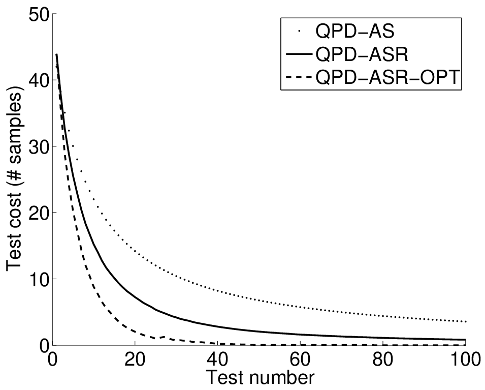
Figure 2 depicts the results. Figure 2(a) shows the mean cost of the ’th test for each implementation. The gradual cost decrease of was already mentioned and discussed by [1]. This results from having the levels of the tests decay faster than assumed as the number of samples grows. This decay can be thought of as a reward for waiting, since users who delay their tests risk losing the novelty of their hypotheses, but are compensated with lower costs. As expected, since and control instead of , they can achieve the requested power using smaller number of samples, hence resulting with lower costs.
Figure 2(b) shows the ratio between the costs required by and by . It shows the mean, median, and the 2.5th and 97.5th percentiles of these ratios over the realizations. Starting after tests the costs of drop to less than one third, on average, than the costs of , and the 97.5th percentile is at .
Figure 2(c) shows the ratio between the costs required by and by . The reduction in cost here is much more dramatic. The cost drops to immediately after the first rejection, and from there on, it usually remains so. This is because the pool fills up with the first reward, and is then generously distributed to subsequent tests. Those tests get so high a level, that no further samples are needed in the database to support the required power. Even though the pool is used generously, the probability of it refilling before running out is so high, that frequently it is enough to supply level allocation for all the remaining tests. All realizations have a cost of from the 78th test onward with . The 97.5th percentile drops to from the 39th test onward.
Comparing the number of rejected hypotheses, all three implementations reject the exact same number of false null hypotheses, on average. Recall that a QPD, regardless of the implementation, serves requests that specify a power requirement, hence all tests in this simulation were performed with power , which explains this identical result (identical realizations of sequences of tests were served by each of the QPD variants). The differences between implementations are in the number of samples present at the ’th test, and the level allocation . and , enjoying the rewards, work with lower number of samples and larger level allocations. These two effects cancel each other to produce the same power, but produce more type-I errors: had type-I errors on average, had , and had . This is expected since controls the , while the other two control .


6 Conclusions
In this paper we discussed sequential procedures for controlling false discovery, and their application to public databases. Specifically, we concentrated on the only known sequential procedure for controlling an -like measure, Alpha Investing, and on the simpler Alpha Spending that controls . We have shown that both can be described as special cases of a more general framework, which offers a trade-off between the level of each test and the reward obtained when the hypothesis is rejected.
We have further shown that from this general framework two additional, novel procedures may be derived, which have practical benefits over existing procedures. The version we termed ERO Alpha Investing is optimal in the sense that, under certain practical assumptions, it tunes the balance between level of the test and the reward such as to maximize the potential for subsequent tests. We have shown it to be significantly more powerful than other Alpha Investing variants in practice. The second, Alpha Spending with Rewards, can be viewed as a cross between Alpha Spending and Alpha Investing. Its practical benefit is that systems that rely on Alpha Spending can be adapted to work with Alpha Spending with Rewards with minimal changes, and enjoy the additional power gained from controlling a less conservative measure of type-I errors.
Finally, we have shown how Alpha Spending with Rewards can be employed to control false discovery in public databases through the framework of Quality Preserving Database (QPD). This demonstrates our previous point, where the QPD framework, previously relying on Alpha Spending, was seamlessly transformed to work with Alpha Spending with Rewards, something that could not have been done with the original Alpha Investing. In addition, this has achieved a significant improvement to the QPD, since replacing with as the controlled measure resulted in costs reduced to practically zero.
This last point is of crucial importance. It implies that a layer for controlling false discovery such as the QPD can be implemented for a freely accessible public database, keeping it almost freely accessible still. The Generalized Alpha Investing procedure and the measure have some drawbacks, most notably the required independence Assumption 2.2, inherited from Alpha Investing. Yet employing it as a method for false discovery control for public databases comes at almost no cost, and it surely offers a huge improvement over the current situation of no false discovery control enforced for public databases to date. All the more so since in the case of public databases, with different research groups researching different aspects of the data, Assumption 2.2 can often be expected to hold approximately.
7 Appendix
7.1 Technical Results and Proofs
Lemma 7.1
Given Assumption 2.2, in the Generalized Alpha Investing Procedure the stochastic process is a sub-martingale with respect to .
We need to show . Note that in analyzing this conditional expectation we will treat , , and as known constants, since given they are deterministically chosen by rule 13.
We will use the abbreviation .
Let us define . Since , and , we can rewrite more explicitly as .
Assuming a true null hypothesis, , we get that . Hence
.
A series of inequalities achieves the desired result:
.
The first inequality follows from Assumption 2.2,
and because
and are nonnegative. The second inequality follows
because by equation 17
,
Assuming a false null hypothesis, , hence
. Now the following series of inequalities will
achieve the desired result:
.
The first inequality follows
from equation 17 since
, and the second inequality
is due to Assumption 2.2.
Theorem 7.2
Clearly, once is set, the optimal choice for is the maximal one allowed by constraint 17. All that remains to show is that has solutions and that they are all indeed optimal. Lemma 7.4 shows the former, and Lemma 7.5 the latter.
Assumption 7.3
Let be the best-power (according to Definition 5), and be the actual probability of rejection for a given , . Then we assume the following: (1) and as functions of are continuous, monotonically non-decreasing, (2) is monotonically non-increasing, (3) is monotonically non-increasing, (4) is monotonically non-increasing.
Lemma 7.4
Given Assumption 7.3, is solvable in the range .
Let us denote . It is enough to show for some . By Assumption 7.3, we know is a continuous function over the range , and clearly . Thus, we can conclude the proof by showing . Since is non-negative and non-decreasing, the limit exists. Let us denote it by . If , then , which implies . If , then by Assumption 7.3, is monotonically non-increasing with . Since , and since the alternative and null hypotheses must be distinct, we must have for some and positive that . Therefore . Since we assumed , we have proved .
Lemma 7.5
Given Assumption 7.3, then for any choice of , and for any , the expression is maximized by setting to be the solution of .
Lemma 7.4 proves is solvable for some . We will now show that maximizes . Using the notation of Assumption 7.3, we can write . Note that brings the two arguments of the operator to equality, therefore it suffices to show that is monotonically non-decreasing with and that is monotonically non-increasing. can be rewritten as . This is monotonically non-decreasing, since are constants, and by Assumption 7.3, is non-decreasing, and is non-decreasing. can be rewritten as . This is monotonically non-increasing, since are constants, and by Assumption 7.3, is non-decreasing, is non-increasing.
Lemma 7.6
Assumption 7.3 holds for Neyman-Pearson tests with continuous distribution functions.
The continuity of and is implied by the underlying continuous distribution functions. Clearly is a non-decreasing function of . is monotonically non-increasing by Lemma 7.8. In Neyman-Pearson tests, is either identical to or to , hence is either the identity function or . In either case it is monotonically non-increasing. A similar argument holds for and for showing is non-decreasing.
Lemma 7.7
For a uniformly most powerful test with a continuous distribution function, a single parameter , and a simple null hypothesis , Assumption 7.3 holds.
The continuity of and is implied by the underlying continuous distribution functions. If the alternative hypothesis is unbounded, then , for which all the required properties involving follow trivially. If the alternative hypothesis is bounded, then the best power is calculated at some extreme point . According to the Neyman-Pearson lemma, the power is identical to the power of a test with a simple alternative , hence Lemma 7.6 proves all the required properties involving . Regarding , it is computed at the actual . If happens to be true, then , and we trivially get all the properties of . Otherwise, a similar argument using the Neyman-Pearson lemma applies.
Lemma 7.8
In Neyman-Pearson tests with continuous distribution functions with level and power , is a monotonically non-increasing function of .
By monotonicity of likelihood ratio implied by the Neyman-Pearson lemma, this is guaranteed.
Procedure Tests True rejects False rejects mFDR Alpha Spending 10.000 0.000 0.046 0.046 Alpha Investing 10.563 0.000 0.047 0.047 Alpha Spending with Rewards (k=1) 10.513 0.000 0.046 0.047 Alpha Spending with Rewards (k=1.1) 11.543 0.000 0.048 0.048 ERO Alpha Investing 17.152 0.000 0.018 0.018
Procedure Tests True rejects False rejects mFDR Alpha Spending 66.000 0.001 0.048 0.048 Alpha Investing 66.678 0.001 0.047 0.047 Alpha Spending with Rewards (k=1) 66.665 0.001 0.047 0.047 Alpha Spending with Rewards (k=1.1) 67.019 0.001 0.049 0.049 ERO Alpha Investing 66.925 0.001 0.056 0.056
Procedure Tests True rejects False rejects mFDR Alpha Spending 200 0.000 0.051 0.051 Alpha Investing 200 0.000 0.052 0.052 Alpha Spending with Rewards (k=1) 200 0.000 0.052 0.052 Alpha Spending with Rewards (k=1.1) 200 0.001 0.054 0.053 ERO Alpha Investing 200 0.001 0.055 0.055
Lemma 7.9
In it holds that .
7.2 Generalized Alpha Investing: Additional Simulation Results
Tables 4, 5, and 6 depict the simulation results with a frequency of false null hypotheses, and effect size of . Regarding number of tests, ERO Alpha Investing significantly out-performed all competitors in both ’constant’ and ’relative’ allocation schemes (paired t-test p-values at most 0.0056), except when compared with the Alpha Spending with Rewards with k=1.1, in the ’relative’ allocation scheme, where the difference was not significant (p-value 0.28). Regarding number of true-rejections, all procedures are performing poorly in these extreme conditions. Hence no significant differences could be found here. Due to the extremely low amount of rejections, the estimation of is inaccurate, hence in some cases it seems above .
8 Acknowledgments
We would like to thank Yoav Benjamini, Marina Bogomolov, Ruth Heller, Daniel Yekutieli, Hani Neuvirth, and the reviewing team for their thoughtful and useful comments. This work was supported by an Open Collaborative Research grant from IBM, and by Israeli Science Foundation grant ISF-1227/09.
References
- [1] Ehud Aharoni, Hani Neuvirth, and Saharon Rosset. The quality preserving database: A computational framework for encouraging collaboration, enhancing power and controlling false discovery. Computational Biology and Bioinformatics, IEEE/ACM Transactions on, 8(5):1431–1437, 2011.
- [2] Yiming Bao, Pavel Bolotov, Dmitry Dernovoy, Boris Kiryutin, Leonid Zaslavsky, Tatiana Tatusova, Jim Ostell, and David Lipman. The influenza virus resource at the national center for biotechnology information. Journal of virology, 82(2):596–601, 2008.
- [3] Yoav Benjamini and Yosef Hochberg. Controlling the false discovery rate: a practical and powerful approach to multiple testing. Journal of the Royal Statistical Society: Series B (Statistical Methodology), pages 289–300, 1995.
- [4] Yoav Benjamini and Daniel Yekutieli. The control of the false discovery rate in multiple testing under dependency. The Annals of Statistics, 29(4):1165–1188, 2001.
- [5] Dean P. Foster and Robert A. Stine. Alpha-investing: a procedure for sequential control of expected false discoveries. Journal of the Royal Statistical Society: Series B (Statistical Methodology), 70(2):429–444, January 2008.
- [6] John Hardy and Andrew Singleton. Genomewide association studies and human disease. New England Journal of Medicine, 360(17):1759–1768, 2009.
- [7] Joel N. Hirschhorn and Mark J. Daly. Genome-wide association studies for common diseases and complex traits. Nature reviews. Genetics, 6(2):95–108, February 2005.
- [8] John PA Ioannidis. Why most published research findings are false. PLoS medicine, 2(8):e124, 2005.
- [9] E. Lander and L. Kruglyak. Genetic dissection of complex traits: guidelines for interpreting and reporting linkage results. Nature genetics, 11(3):241–247, November 1995.
- [10] Adam C. Naj, Gyungah Jun, Gary W. Beecham, Li-San S. Wang, Badri Narayan N. Vardarajan, et al. Common variants at MS4A4/MS4A6E, CD2AP, CD33 and EPHA1 are associated with late-onset Alzheimer’s disease. Nature genetics, 43(5):436–441, May 2011.
- [11] Hani Neuvirth, Uri Heinemann, David Birnbaum, Naftali Tishby, and Gideon Schreiber. Promateus–an open research approach to protein-binding sites analysis. Nucleic acids research, 35(suppl 2):W543–W548, 2007.
- [12] Soo-Yon Rhee, Matthew J Gonzales, Rami Kantor, Bradley J Betts, Jaideep Ravela, and Robert W Shafer. Human immunodeficiency virus reverse transcriptase and protease sequence database. Nucleic acids research, 31(1):298–303, 2003.
- [13] Robert John Simes. Publication bias: the case for an international registry of clinical trials. Journal of Clinical Oncology, 4:1529–1541, 1986.
- [14] John D Storey. A direct approach to false discovery rates. Journal of the Royal Statistical Society: Series B (Statistical Methodology), 64(3):479–498, 2002.
- [15] Hua Tang, Jie Peng, Pei Wang, Marc Coram, and Li Hsu. Combining multiple family-based association studies. BMC Proceedings, 1(Suppl 1):S162, 2007.
- [16] Edwin J. C. G. van den Oord and Patrick F. Sullivan. False discoveries and models for gene discovery. Trends in Genetics, 19(10):537–542, 2003.
- [17] Wellcome Trust Case Control Consortium. Genome-wide association study of 14,000 cases of seven common diseases and 3,000 shared controls. Nature, 447(7145):661–678, June 2007.
- [18] Wellcome Trust Case Control Consortium. Genome-wide association study of CNVs in 16,000 cases of eight common diseases and 3,000 shared controls. Nature, 464(7289):713–720, April 2010.