Distinguishing between lepton number violating scalars at the LHC

At a hadron collider $H^{\pm\pm}$ are mainly pair produced through the $s$-channel exchange of photons and $Z$ bosons, being their electro-weak gauge couplings obtained from the corresponding kinetic term $(D_{\mu}H)^{\dagger}(D^{\mu}H)$. They can be also be produced singly through the s-channel exchange of $W$ bosons if $T\neq 0$ . Both cross-sections are of electro-weak size but vary with the multiplet $H^{\pm\pm}$ belongs to [27]. For instance, they grow with $T$ for multiplets with components of charge at most $Q=T_{3}+Y=2$ (that is, with $T^{H^{++}}_{3}=T$). They can be also produced by vector boson fusion, which can be considered to be a next-order correction and will be neglected here ⁶⁶ 6 Single doubly-charged production through vector boson fusion can be eventually at the LHC reach for rather bizarre models evading the stringent electro-weak constraints on the VEV of the neutral scalar partner of the doubly-charged scalar boson [37, 38]. In this case the doubly-charged scalar only decays into W pairs, and then it does not resonate in the di-leptonic channel.. Although the vector boson fusion contribution grows with the $H^{\pm\pm}$ mass, it is smaller than the one mediated by the s-channel electro-weak gauge boson exchange by almost an order of magnitude for multiplets satisfying $T^{H^{++}}_{3}=T$ and doubly-charged scalar masses below the TeV; details will be provided in a forthcoming publication. In any case, the corresponding events have two extra jets with relatively large pseudo-rapidity which provide an extra handle to separate them.

Our purpose here is to review how to determine the doubly-charged scalar pair production cross-section, and thus measure $T^{H^{++}}_{3}$, using only four lepton final states. We concentrate for simplicity on the case $T^{H^{++}}_{3}=T$, ⁷⁷ 7 Models also including scalars with larger electric charges can produce even more striking signals [39, 40, 41]. In any case, we assume that mass splittings within multiplets due to mixing with other scalars are small, and can be neglected [42, 43]. thus restricting $T=0,1/2,1,3/2,2$.

We are interested in measuring the total cross-section $\sigma$ in order to determine the isospin of the multiplet the doubly-charged scalar belongs to. However, this cannot be done using a single decay mode because the corresponding number of signal events also depends on the $H^{\pm\pm}$ branching ratio into this mode, which is in principle unknown. Thus, we must determine the number of events for each channel and sum them appropriately taking into account the different efficiencies to estimate the total cross section. What can be done using only events with four charged leptons, properly sampled, and Eq. (7) in Ref. [27] is to measure

where $\sigma_{ab}=(2-\delta_{ab})\sigma z_{a}z_{b}$ is the $H^{\pm\pm}$ pair production cross-section into $ab$, with $z_{a}\equiv Br(H\rightarrow a)$ the $H$ branching ratio into $a$ and $\sum_{a=ll,l\tau,\tau\tau,WW}z_{a}=1$.

In practice we proceed as follows. We select events with four charged leptons of the first two families with zero total electric charge, plus possibly missing transverse momentum, and require that at least one same-sign pair $l_{1}l_{2}$ reconstructs the scalar mass within $\pm 40$ GeV. (See Table 1 for a summary of the main cuts.)

These events are then separated into three disjoint sets depending on the category associated to the other like-sign pair: $ll,l\tau$ and $\tau\tau+WW$. We denote by $ll$ those events resulting from the decay of the second doubly-charged scalar into two leptons of the first two families, and hence, those with the second like-sign lepton pair $l_{3}l_{4}$ also reconstructing the scalar mass within $\pm 40$ GeV. For the remaining events we assume that $l_{3}$ and $l_{4}$ are products of semileptonic tau decays, and distribute the transverse missing momentum of the event between both tau leptons with the requirement that their momenta align along the momentum of the corresponding product charged-lepton momentum it decays to: $xp_{\tau}^{\mu}=p_{l}^{\mu}$, with $0<x<1$. Then, we identify the event with the second scalar decaying into a lepton of the first two families and a tau lepton, $l\tau$, as those fulfilling that the fraction momentum of the most energetic of the two leptons not reconstructing the scalar mass, which we name $l_{3}$, ($x_{3}$) is larger than 0.8. The other events are classified as resulting from the decay of the second scalar into two tau leptons or two gauge bosons, $\tau\tau+WW$.

Figures 1, 2 and 3 prove the usefulness of the procedure. Indeed,

Figure 1 shows the like-sign di-lepton invariant mass for the lepton pair which provides the poorest reconstruction of the doubly-charged scalar mass and for its four decay modes: $H^{\pm\pm}\rightarrow l_{3}^{\pm}l_{4}^{\pm}$, $H^{\pm\pm}\rightarrow l_{3}^{\pm}\tau^{\pm}\rightarrow l_{3}^{\pm}l_{4}^{\pm}{\cancel{p}}_{T}$, $H^{\pm\pm}\rightarrow\tau^{\pm}\tau^{\pm}\rightarrow l_{3}^{\pm}l_{4}^{\pm}{\cancel{p}}_{T}$, and $H^{\pm\pm}\rightarrow W^{\pm}W^{\pm}\rightarrow l_{3}^{\pm}l_{4}^{\pm}{\cancel{p}}_{T}$. The separation of the first sample is obtained simply requiring $m_{l_{3}^{\pm}l_{4}^{\pm}}$ to be in between $m_{H^{\pm\pm}}\pm 40$ GeV. In Figure 2 we plot the momentum fraction assigned to the most energetic lepton of the second like-sign pair for the former four types of scalar decays. As can be observed, $x_{3}\geq 0.8$ provides a rather clean separation of the first two decay modes from the last two. The different distributions reflect the fact that the leading lepton tends to be the one which is not a decay product of a $\tau$ or a $W$, and thus with $x_{3}\sim 1$. In order to further reduce the contamination we also require $x_{3}\leq 0.7$ for $\tau\tau+WW$ events. Finally, Figure 3 makes it clear that separating $\tau\tau$ and $WW$ decays is rather inefficient. However, what further justifies not doing this at this stage, for evaluating the total pair production cross-section, is that the efficiency $\epsilon$ for evaluating the cross-sections of both types of processes is rather similar, allowing to treat both together consistently.

Actually, in order to measure the total pair production cross-section using Eq. (1), we have to estimate the efficiency for each process. From our Monte Carlo simulations we have calculated the efficiency for each subsample including the corresponding branching ratios, obtaining: $\epsilon_{llll}=0.6,\epsilon_{lll\tau}=0.09$ and $\epsilon_{ll\tau\tau}=\epsilon_{llWW}=0.02$, respectively. Then, counting the number of events of each of the three subsets and dividing by the corresponding efficiency, we can measure the doubly-charged scalar pair production cross-section, once the integrated luminosity $\cal L$ is known. In Figure 4 we plot the statistical error for such a determination for several $H^{\pm\pm}$ branching ratio assumptions and the five multiplet assignments $T_{Y}$ discussed above.

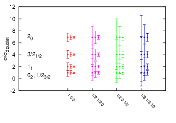
The cross-sections are correctly reproduced because they are an input, but what matters is with which precision can we measure them in order to distinguish between different multiplet assignments. We draw statistical errors including the effect of SM backgrounds for three different integrated luminosities: 100, 300 and 3000 fb^-1. (For example, we find $\sim 50$ background events for ${\cal L}=300$ fb^-1 with four charged leptons adding to zero total electric charge and a same-sign pair reconstructing the $H^{\pm\pm}$ mass within 40 GeV.) We fix four definite sets of doubly-charged scalar branching ratios: $(z_{ll},z_{l\tau},z_{\tau\tau}+z_{WW})=$ $(1,0,0)$, $(1/2,1/2,0)$, $(1/2,0,1/2)$, $(1/3,1/3,1/3)$, being higher the precision with $z_{ll}>z_{l\tau}>z_{\tau\tau}+z_{WW}$ . This means worsening when worse is our ability to reconstruct the $H^{\pm\pm}$ mass.

As can be observed in Figure 4, there is no apparent difference between the singlet and doublet cases because their neutral cross-sections are rather similar, but this is not so for the charged ones as there is no charged-boson exchange graph in the singlet case [27]. Thus, the associated production of doubly-charged scalars can be used to discriminate between these two multiplets. If there is a significant excess of events compatible with $H^{\pm\pm}H^{\mp}$, the singlet hypothesis will be automatically ruled out. However, to establish whether this is the case must be carefully assessed because the observation of only three leptons in the final state does not uniquely characterize this (charged-current) process. For instance, pair produced doubly-charged scalars decaying into $l^{\pm}l^{\pm}l^{\mp}\tau^{\mp},l^{\pm}l^{\pm}\tau^{\mp}\tau^{\mp}$ or $l^{\pm}l^{\pm}W^{\mp}W^{\mp}$ can also produce only three leptons if one $\tau$ or $W$ decays hadronically. Therefore, we need to rely on extra variables in order to forbid these (neutral-current) contributions. Two discriminators appear to be most convenient: the missing transverse momentum, ${\cancel{p}}_{T}$, which is larger in single $H^{\pm\pm}$ production than in $l^{\pm}l^{\pm}l^{\mp}\tau^{\mp}$ events with $\tau^{\mp}$ decaying hadronically, which allows to separate both contributions; and the transverse invariant mass of the opposite-sign lepton and the missing transverse momentun, $m_{T}(l^{\pm}_{3}{\cancel{p}}_{T})$, which peaks near the $H^{\pm}$ mass in the charged-current process, as shown in Figure 5.

It is apparent from this figure that a cut on $m_{T}>250$ GeV suppresses the neutral $\tau\tau$ and $WW$ contributions quite efficiently.

Although it is neither efficient nor necessary to separate $\tau\tau$ from $WW$ events in order to determine the total $H^{\pm\pm}$ pair production cross-section in Eq. (1), one must attempt to do it in order to establish or not the violation of LN at the LHC. This separation makes use of the invariant mass distribution in Figure 3: $WW$ events are defined as those outside a wide enough interval around the $H^{\pm\pm}$ mass. Reconstructed $\tau\tau$ events near the doubly-charged scalar mass are interpreted as genuine $\tau\tau$ decays. For the events left, and interpreted as $WW$ decays, one must also check that the assignment is consistent with such a $H^{\pm\pm}$ decay. One can also check the consistency with the excess of events resulting from the semi-leptonic decay of the $WW$ pair, but this has other backgrounds, too, and will be discussed elsewhere.

References

- (1) G. Aad et al. [ATLAS Collaboration], Phys. Lett. B 716 (2012) 1 [arXiv:1207.7214 [hep-ex]].
- (2) S. Chatrchyan et al. [CMS Collaboration], Phys. Lett. B 716 (2012) 30 [arXiv:1207.7235 [hep-ex]].
- (3) W. -Y. Keung and G. Senjanovic, Phys. Rev. Lett. 50 (1983) 1427.
- (4) J. Schechter and J. W. F. Valle, Phys. Rev. D 25 (1982) 2951.
- (5) K. S. Babu and C. N. Leung, Nucl. Phys. B 619 (2001) 667 [hep-ph/0106054].
- (6) K. -w. Choi, K. S. Jeong and W. Y. Song, Phys. Rev. D 66 (2002) 093007 [hep-ph/0207180].
- (7) J. Engel and P. Vogel, Phys. Rev. C 69 (2004) 034304 [nucl-th/0311072].
- (8) A. de Gouvea and J. Jenkins, Phys. Rev. D 77 (2008) 013008 [arXiv:0708.1344 [hep-ph]].
- (9) F. del Aguila, A. Aparici, S. Bhattacharya, A. Santamaria, J. Wudka and , JHEP 1206 (2012) 146 [arXiv:1204.5986 [hep-ph]].
- (10) F. del Aguila, A. Aparici, S. Bhattacharya, A. Santamaria and J. Wudka, arXiv:1305.4900 [hep-ph].
- (11) P. Minkowski, Phys. Lett. B 67 (1977) 421.
- (12) T. Yanagida, Conf. Proc. C 7902131 (1979) 95.
- (13) M. Gell-Mann, P. Ramond and R. Slansky, Conf. Proc. C 790927 (1979) 315 [arXiv:1306.4669 [hep-th]].
- (14) S. L. Glashow, NATO Adv. Study Inst. Ser. B Phys. 59 (1980) 687.
- (15) R. N. Mohapatra and G. Senjanovic, Phys. Rev. Lett. 44 (1980) 912.
- (16) T. Han and B. Zhang, Phys. Rev. Lett. 97 (2006) 171804 [hep-ph/0604064].
- (17) F. del Aguila, J. A. Aguilar-Saavedra and R. Pittau, JHEP 0710 (2007) 047 [hep-ph/0703261].
- (18) A. Atre, T. Han, S. Pascoli and B. Zhang, JHEP 0905 (2009) 030 [arXiv:0901.3589 [hep-ph]].
- (19) F. del Aguila, J. de Blas and M. Perez-Victoria, Phys. Rev. D78 (2008) 013010 [arXiv:0803.4008 [hep-ph]].
- (20) R. E. Marshak and R. N. Mohapatra, In *Coral Gables 1980, Proceedings, Recent Developments In High-energy Physics*, 277-287
- (21) J. Schechter and J. W. F. Valle, Phys. Rev. D 22 (1980) 2227.
- (22) T. P. Cheng and L. -F. Li, Phys. Rev. D 22 (1980) 2860.
- (23) S. Chatrchyan et al. [CMS Collaboration], Eur. Phys. J. C 72 (2012) 2189 [arXiv:1207.2666 [hep-ex]].
- (24) G. Aad et al. [ATLAS Collaboration], Eur. Phys. J. C 72 (2012) 2244 [arXiv:1210.5070 [hep-ex]].
- (25) A. Hektor, M. Kadastik, M. Muntel, M. Raidal and L. Rebane, Nucl. Phys. B 787 (2007) 198 [arXiv:0705.1495 [hep-ph]].
- (26) F. del Aguila and J. A. Aguilar-Saavedra, Nucl. Phys. B813 (2009) 22–90, [arXiv:0808.2468 [hep-ph]].
- (27) F. del Aguila, M. Chala, A. Santamaria and J. Wudka, arXiv:1305.3904 [hep-ph].
- (28) A. Zee, Nucl. Phys. B 264 (1986) 99.
- (29) K. S. Babu, Phys. Lett. B 203 (1988) 132.
- (30) F. del Aguila, A. Aparici, S. Bhattacharya, A. Santamaria and J. Wudka, JHEP 1205 (2012) 133 [arXiv:1111.6960 [hep-ph]].
- (31) M. Gustafsson, J. M. No and M. A. Rivera, Approved for Phys.Rev.Lett.,2013 [arXiv:1212.4806 [hep-ph]].
- (32) J. F. Gunion, C. Loomis and K. T. Pitts, eConf C 960625 (1996) LTH096 [hep-ph/9610237].
- (33) V. Rentala, W. Shepherd and S. Su, Phys. Rev. D 84 (2011) 035004 [arXiv:1105.1379 [hep-ph]].
- (34) M. Aoki, S. Kanemura and K. Yagyu, Phys. Lett. B 702 (2011) 355 [Erratum-ibid. B 706 (2012) 495] [arXiv:1105.2075 [hep-ph]].
- (35) K. Yagyu, arXiv:1304.6338 [hep-ph].
- (36) S. Kanemura, K. Yagyu and H. Yokoya, arXiv:1305.2383 [hep-ph].
- (37) C. -W. Chiang, T. Nomura and K. Tsumura, Phys. Rev. D 85 (2012) 095023 [arXiv:1202.2014 [hep-ph]].
- (38) C. Englert, E. Re and M. Spannowsky, arXiv:1306.6228 [hep-ph].
- (39) K. S. Babu, S. Nandi and Z. Tavartkiladze, Phys. Rev. D 80 (2009) 071702 [arXiv:0905.2710 [hep-ph]].
- (40) G. Bambhaniya, J. Chakrabortty, S. Goswami and P. Konar, arXiv:1305.2795 [hep-ph].
- (41) R. Franceschini and R. N. Mohapatra, arXiv:1306.6108 [hep-ph].
- (42) A. G. Akeroyd and S. Moretti, Phys. Rev. D 84 (2011) 035028 [arXiv:1106.3427 [hep-ph]].
- (43) M. Aoki, S. Kanemura and K. Yagyu, Phys. Rev. D 85 (2012) 055007 [arXiv:1110.4625 [hep-ph]].
- (44) J. Alwall, M. Herquet, F. Maltoni, O. Mattelaer and T. Stelzer, JHEP 1106 (2011) 128 [arXiv:1106.0522 [hep-ph]].
- (45) N. D. Christensen and C. Duhr, Comput. Phys. Commun. 180 (2009) 1614 [arXiv:0806.4194 [hep-ph]].
- (46) M. L. Mangano, M. Moretti, F. Piccinini, R. Pittau and A. D. Polosa, JHEP 0307 (2003) 001 [hep-ph/0206293].
- (47) T. Sjostrand, S. Mrenna and P. Z. Skands, JHEP 0605 (2006) 026 [hep-ph/0603175].
- (48) S. Ovyn, X. Rouby and V. Lemaitre, arXiv:0903.2225 [hep-ph].