Demography-adjusted tests of neutrality based on genome-wide SNP data
Abstract
Tests of the neutral evolution hypothesis are usually built on the standard null model which assumes that mutations are neutral and population size remains constant over time.
However, it is unclear how such tests are affected if the last assumption is dropped.
Here, we extend the unifying framework for tests based on the site frequency spectrum, introduced by Achaz and Ferretti, to populations of varying size.
A key ingredient is to specify the first two moments of the frequency spectrum.
We show that these moments can be determined analytically if a population has experienced two instantaneous size changes in the past.
We apply our method to data from ten human populations gathered in the genomes project,
estimate their demographies and define demography-adjusted versions of Tajima’s , Fay & Wu’s , and Zeng’s .
The adjusted test statistics facilitate the direct comparison between populations and they show that most of the differences among populations seen in the original tests can be explained by demography. We carried out
whole genome screens for deviation from neutrality and identified candidate regions of
recent positive selection. We provide track files with values of the adjusted and original tests
for upload to the UCSC genome browser.
Keywords: Single nucleotide polymorphism, infinite-sites model, site frequency spectrum, bottleneck, coalescent approximation.
I Introduction
In natural populations, genetic diversity is shaped not only by population genetic forces such as drift and natural selection, but also by geographic structure and demographic history. Many statistical tests to identify genome regions affected by natural selection have been proposed in the past, such as iHS [27], XP-EHH [26] as well as Tajima’s [24], Fay&Wu’s [9], and Zengs’s [29]. Tests of neutrality have frequently been used to search for signatures of selection in the human genome [4, 23, 5, 21, 27]. However, distinguishing selection from demographic effects in genomic data remains a challenge [4, 23]. In this paper, we focus on tests based on the shape of the site frequency spectrum, such as Tajima’s , Fay&Wu’s , and Zeng’s . As examples, we show in Fig. 1 (upper panels) genome-wide values of these tests for a European (CEU), Asian (CHB), and African human population (YRI) in the genomes project dataset [18]. As Fig. 1 (upper panels) shows, the distributions of the tests differ substantially between different populations. To which extent do these differences arise from differences in demographic histories of the populations? In order to answer this question, it is necessary to eliminate the effects of demographies on the values of tests. In this study, we achieve this by adjusting the site frequency spectrum of tests of neutrality for the deviation of population demographies from constant size. Thus, we modify tests of neutrality by directly integrating demographies into them. We refer to such modified tests as demography-adjusted. When demography corresponds to constant population size, demography-adjusted tests reduce to the tests defined for the standard Wright-Fisher model, hereafter referred to as original tests.
The distributions of demography-adjusted tests are similar to the distributions of the corresponding original tests computed under the standard null model. Consequently, demography-adjusted tests significantly simplify a direct comparison of the values of tests between different populations by emphasising the relevant differences. Examples are given in Fig. 1 (lower panels), where we show the distributions of our demography-adjusted Tajima’s , Fay&Wu’s , and Zeng’s for the populations CEU, CHB, and YRI. As this figure suggests, most of the differences in the distributions of the tests between human populations arise from their distinct underlying demographies.
Since human demographies are unknown, it is necessary to estimate them. As suggested by Nielsen [20] (see also Adams and Hudson [3]), we apply a maximum likelihood method to genome-wide single nucleotide polymorphisms (SNPs). As an approximation for the demographies of human populations we use a simplified model with two instantaneous population size changes in the past, as proposed before [3, 17, 23]. This model is characterized by four unknown parameters. It has the appealing property to yield exact analytical expressions for the first two moments of the site frequency spectrum (SFS). These are required to formulate our demography-adjusted tests of neutrality and they are explicitly derived in this paper.
The error in the estimate of demographic parameters depends on the noise in the genome-wide SFS, thus on the number of SNPs used for the estimation. We analyse the sensitivity of demography-adjusted tests by using coalescent simulations. On the basis of two reference demographies with two population-size changes in the past, we determine the number of SNPs required for reliable adjustment of the tests.
The populations CEU, CHB, and YRI are only three exemplary populations chosen from a set of ten populations analysed in this study by means of demography-adjusted tests. Assuming a piecewise constant demographic model, we find that Europeans and Asians went through a recent population bottleneck, which is in agreement with Adams and Hudson [3] and Marth et al. [17]. In contrast, the African populations either experienced two population-size expansions (ASW, again in agreement with Adams and Hudson [3] and Marth et al. [17]), or an ancient expansion, followed by a recent population-size decline (LWK, YRI).
Our results further show that demography-adjustment of SFS-based tests is essentially reflected in an affine linear transformation of the test statistic. Consequently, the genomic regions recognized to be under selection by the adjusted tests strongly overlap with the originally detected regions. However, our adjusted tests permit a direct comparison of results from different populations with different demographies.
We provide original and adjusted tests values as BED-files, formatted for upload to the UCSC genome browser.


II Materials and methods
II.1 Demographic model
We assume a piecewise constant demography with two population-size changes in the past as illustrated in Fig. 2. When and the demography represents a population bottleneck. The model of piecewise constant demographies with two population-size changes in the past was considered before [3, 17, 23] to capture the main events of the human out-of-Africa expansion [6, 22, 16, 25, 7].
II.2 Demography-adjusted tests of neutrality
Tajima [24] introduced a test of neutrality which compares two estimators of the scaled mutation rate , with denoting diploid population size, mutation rate per site, per chromosome, per generation, and the number of sites in the genomic sequence. If mutations are neutral, these two estimators have the same expected values. A significant difference between them indicates a violation of the null assumptions, i. e. either the population size is varying, or mutations are not neutral (or both). Several other tests of neutrality, relying on the same idea and on the same null model, have been proposed since (Fu and Li [14], Fay and Wu [9], Zeng et al. [29], Achaz [1]). Achaz [2] showed that estimators of in any of these tests can be expressed as linear combinations of the SFS, and as instances of a single general formula (see Eq. (8) in Achaz [2]).
We show that this can be further generalised to include demographies with varying population size. Following the notation introduced by Achaz [2] and Ferretti et al. [10], we write the null site frequency spectrum in the form . Here is the expected total branch length of lineages in the gene genealogical tree of the sample that have exactly leafs. It depends on the sample size and the parameters of the demography, but not on . It follows that in a sample of size , the SFS provides unbiased estimators . In fact, any linear combination of can be used as an estimator of :
| (1) |
where are the weights satisfying . All tests mentioned above compare two different such estimators and are determined only by the difference of the corresponding weights (listed in Table 1 and 2 of Achaz [2]).
It follows from Eq. (1) that a demography-adjusted test of neutrality, denoted by below, takes the form [10, their suppl. Eq. (20)]:
| (2) |
The denominator in Eq. (2) for a constant population size is given by Achaz [2, his Eq. (9)]. For a varying population size, we calculate analogously (see Appendix Appendix A: The denominator of demography-adjusted tests of neutrality based on the SFS):
| (3) |
where for , and , as defined in Fu [12]. Note that, according to its definition, does not depend on . In the constant population-size case, it is a function of sample size (see Fu [12]), and for a non-constant demography it is a function of and of the parameters of the demography.
As Eq. (3) shows, an estimate of and of is needed to calculate the variance. Tajima [24] used the estimator (where is the number of segregating sites). We extend this definition to an arbitrary null spectrum by setting . We find that an unbiased estimate of based on is given by (see Appendix Appendix A: The denominator of demography-adjusted tests of neutrality based on the SFS)
| (4) |
Here, and are given by
| (5) |
For constant population size and reduce to
| (6) |
It is known that estimation of by is efficient (i. e. the estimator has minimal variance) for small values of [13]. One can show that this holds for our extended version of as well. In fact, the estimator can become efficient even for high values of , if recombination is taken into account. We note that it is common practise to apply tests, such as Tajima’s , to recombining sequences [4, 23, 5] although their derivation neglects recombination.
In our genome scan we encounter rather high values of in the range of . In this case the first summand in Eq. (3) can be neglected. Hence, Eq. (2) can be approximated by
| (7) |
and the adjustment of the tests to demography with varying population size can be interpreted as a combination of a modified weighting (via ) and scaling (via and ), yielding an affine linear transformation.
Note, that our adjusted tests co-incide with the original ones if population size is constant. In this case, expressions for and have been explicitly derived by Fu [12]. In case of varying population size, the corresponding expressions are, in general, unknown. For a piecewise constant demography, Marth et al. [17] derived an expression for the first moment of the SFS. In this study, we use results of Fu [12] and of Eriksson et al. [8] (see also Zivkovic and Wiehe [30]) to compute the second moment of the SFS under a piecewise constant demography shown in Fig. 2. We remark, that this can be done in the same way for the folded SFS (FSFS), i.e. when data cannot be polarized. The details and the corresponding formulae for the demographic model shown in Fig. 2 are given in Appendix Appendix B: The first two moments of the SFS.
II.3 Estimating demographic parameters using the SFS
We use the analytical expressions for the moments of the SFS under a given demography to compute maximum likelihood (ML) estimates of the parameters of our demographic model. We follow a similar approach as described in Adams and Hudson [3], namely we calculate the expected SFS for a large set of plausible parameters and choose the parameters with highest likelihood, given the data. If SNPs are assumed to be uncorrelated, the SFS counts are multinomially distributed (conditional on the total number of SNPs ), with the parameters given by the expected values of [20, 3].
Similarly, the probability to observe the FSFS in a sample of polymorphic sites is multinomial with
| (8) |
In this case, the parameters are given by:
| (9) |
As mentioned in the previous subsection, the expression for (and thus for ) under the model shown in Fig. 2 is given in Appendix Appendix B: The first two moments of the SFS.
It is known that different demographies can lead to exactly the same SFS [19]. Hence, cases exist in which it is difficult to distinguish the underlying demographies by their spectra. In order to obtain an estimate for the minimum number of SNPs necessary for reliable inference, we use coalescent simulations to generate SFSs under two different demographic histories with two population-size changes in the past (see Fig. 3). Reconstruction of the ancestral allele via an outgroup is prone to mis-specification, which can substantially bias demography estimation. We therefore used the folded SFSs (FSFSs) for demography estimation, which is independent of the ancestral allele. We simulated independent gene genealogies with , and . For such a small value of , genealogies rarely contain more than one mutation. For each demography, we determine three resulting FSFSs, one containing SNPs, one with SNPs, and one with SNPs (see circles in Fig. S1 in Supplementary material). To obtain the FSFSs in a way consistent with practical data sampling, we randomly select exactly one SNP from randomly chosen genealogies having mutations. Using such spectra, we compute ML-parameters of demographies with two population-size changes in the past. We note that, under the model considered, there are four unknown parameters to be determined. Upon scaling the parameters of the model (, , , , ) by the present population size , the unknown parameters actually are the scaled population sizes (), and the scaled times such that (). For the given parameters , , , and , the probabilities can be computed using Eqs. (22)-(24) in Appendix Appendix B: The first two moments of the SFS. Note that the ML-estimation does not depend on the parameter , as Eq. (9) shows. The ML-demographies are found by computing for a set of candidate parameters: the logarithms of candidate population sizes , and are taken from a grid within the interval , and the logarithms of candidate times , and are taken from a grid within the interval (in both cases successive points are equally spaced by units). Thus, for each population we test in total combinations of the four unknown demographic parameters. The results are shown in Section III.
We apply this procedure to the FSFSs of ten human populations (see Table 1) to estimate the parameters of the corresponding piecewise constant demographies with two population-size changes in the past (Fig. 2). Data were taken from the genomes project [18], version of the release of integrated variant calls from April th, . Variants were filtered by variant type “SNP” (i.e. indels excluded). From each population, four (possibly overlapping) subsamples of individuals were drawn. We used only SNPs from intergenic regions.
| Population | Sample | |
|---|---|---|
| CEU | CEPH individuals | 85 |
| FIN | Finnish in Finland | 93 |
| GBR | British from England and Scotland | 89 |
| TSI | Toscani in Italia | 98 |
| CHB | Han Chinese in Beijing, China | 97 |
| CHS | Han Chinese South, China | 100 |
| JPT | Japanese in Tokyo, Japan | 89 |
| ASW | African ancestry in Southwest USA | 61 |
| LWK | Luhya in Webuye, Kenya | 97 |
| YRI | Yoruba in Ibadan, Nigeria | 88 |
As explained above, in order to use the analytical formulae for parameter estimation, SNPs must be uncorrelated, i. e. unlinked. On the other hand, a large amount of SNPs is necessary to render the demography estimation reliable. As a compromise we collect the SNPs in the following way: from each of the 4 subsamples of individuals we draw randomly SNPs with the condition that the minimal physical distance between any pair of SNPs is base pairs ( kb). This is repeated times for each subsample to obtain in total random spectra. We perform the ML-estimation for each population by using the average of these spectra. Results are shown in Section III.


II.4 Whole-genome scans with demography-adjusted tests of neutrality
First, we investigate with simulations the error introduced by demography inference. We simulate independent gene genealogies under two idealized demographies roughly representing the populations CEU and YRI, shown in Fig. 3b, d by black lines (recent bottleneck in b, and past population-size expansion followed by a recent decline in d). We performed coalescent simulations with , corresponding to the values in our genome scan. For each gene genealogy, we compute the distribution of Tajima’s adjusted to the actual demography, as well as to the estimated demography, and we compare the two.
We perform genome wide computation of Tajima’s , Fay Wu’s and Zeng’s using the approach by Carlson et al. [5]. We calculate the tests in a sliding window of size kb and step size kb. Windows containing less than SNPs were ignored and we collected about data points. For the tests of Fay Wu, and of Zeng it is necessary to know the ancestral allele. This information was obtained through a -way alignment of humans and five other primates and is included into the genomes data. In order to detect putative regions under selection, we distinguished so-called “contiguous regions of Tajima’s reduction (CRTR)”. As in Carlson et al. [5] we define them as a genomic region of at least 20 consecutive windows, of which at least 75 show a Tajima’s belonging to the lowest overall values.
III Results
III.1 Test of the maximum likelihood procedure
In Fig. 3a, c we show by black lines the analytically computed scaled FSFSs under a recent bottleneck (a), that is under a past population-size expansion followed by a recent decline (c). The spectra are scaled so that in the constant population-size case one obtains a constant value (independent of ) equal to (dashed lines in Fig. 3a, c). The demography estimation is based on the spectra obtained using coalescent simulations with , or , or SNPs (see blue, green, and red circles in Fig. S1b, d in Supplementary material). By comparing the actual underlying histories to the estimated ones, we find that our ML-procedure works well when using spectra with SNPs.
In Fig. 4 we show the distributions of Tajima’s adjusted to the ML-demographies shown in Fig. 3b, d (blue, and green circles). For comparison, we also show the distributions of Tajima’s adjusted to the corresponding actual demographies (grey regions), and to the constant population-size history, i. e. original Tajima’s (black circles). Fig. 4a and b show the results based on SNPs, and Fig. 4c and d show the results based on SNPs. Our results show that Tajima’s adjusted to the ML-demography coincides well with Tajima’s adjusted to the actual underlying history if the demography estimation is performed using SNPs (compare Fig. 4a and c to Fig. 4b and d). Note, that while we adjust the tests for the first two moments, demography influences also higher moments. This leads to a skewness of the adjusted distributions versus the neutral ones as noticed already by Zivkovic and Wiehe [30].
III.2 Estimated human demographies
| Population | Intra-sample average | SD | Inter-sample average | SD |
|---|---|---|---|---|
| CEU | 2029 | 14.0 | 2043 | 25.0 |
| FIN | 1894 | 16.9 | 1896 | 18.9 |
| GBR | 2062 | 9.4 | 2064 | 17.1 |
| TSI | 2165 | 9.5 | 2165 | 9.2 |
| CHB | 2039 | 16.2 | 2031 | 23.9 |
| CHS | 2048 | 13.3 | 2036 | 52.2 |
| JPT | 1955 | 10.8 | 1944 | 16.7 |
| ASW | 2837 | 7.3 | 2833 | 23.0 |
| LWK | 2665 | 15.3 | 2652 | 71.6 |
| YRI | 2352 | 6.6 | 2350 | 24.4 |
We now analyze the reliability of the obtained frequency spectra of the human populations. Table 2 gives an overview of the variation contained in the empirical FSFSs of the populations. We focus on singletons (mutations of size ) since they represent the most distinctive part of the frequency spectrum between populations. For each population we compare multiple SNP samplings of the same subsample of individuals to those of different subsamples of the same size. It can be seen that our procedure to extract SNPs essentially grasps the information contained in a specific subsample, since we find only minor changes by repeating it on the same sample. The variation between different subsamples, which is highest for LWK, may hint at some substructure in a given population. The populations CHB, CHS, GBR and CEU are not distinguishable by their amount of singletons (see Table 2), but they become distinguishable when doubletons are taken into account (not shown). The difference between CHB and CHS remains small, though, and their whole frequency spectra are the most similar ones among all populations.
Our demography estimation shows (see Fig. 5 and Table S1 in Supplementary material) that the FSFSs of the non-African populations are consistent with a population bottleneck. By contrast, the FSFS of the African population ASW is consistent with two population-size expansions, and the FSFSs of LWK and YRI are consistent with an inverse bottleneck.
III.3 Neutrality tests adjusted to the estimated human demographies
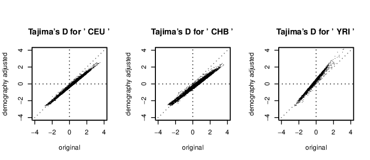
Figure 6 shows the original test values of Tajima’s D plotted against the adjusted ones for nonoverlapping windows of size kb. The inclusion of demography into the tests basically results in an affine linear transformation of the test values (coefficient of determination ). Since is large ( for almost all regions), this observation fits our theoretical result of Eq. (7). The residuals of a linear regression of the adjusted on the original values are approximately normally distributed with standard deviation of . This suggests that the scattering observed in the figure should be interpreted as noise and not as a biological phenomenon. Some of the “outliers” appear to be due to windows containing very few SNPs. However, on the other hand, we notice that the residuals of different subsamples are correlated () for the same population, but not for different populations. This hints at a possible systematic effect. The linearity implies that the empirical quantiles of the test statistics are unaffected by the adjustment.


III.4 Identifying candidate regions of positive selection
We compare Tajima’s between the four subsamples of the same population. The coefficient of determination is about in all populations. The highest correlation between samples from different populations show CHB with CHS (), and CEU with GBR (). The lowest correlation show LWK or YRI compared with the Asian populations (). We find that CRTRs vary considerably among subsamples of the same population. We therefore add a condition and require the test statistic of a particular window to be in the -quantile simultaneously for all four subsamples. From these windows we construct CRTRs as described above. The additional constraint reduces the number of CRTRs by more than . For the populations CEU, CHB and YRI the obtained regions are depicted in Figure 7. We obtain ( for adjusted test values) CRTRs for population CEU, () for CHB and () for YRI, respectively. Carlson et al. [5], using the SNP array data available at that time, obtained CRTRs for the African, for the European and for the Chinese population samples which only partially overlap with ours. These differences are caused most likely by the distinct population samples used. In the supplement we list CRTRs of all 10 populations. If the relation between original and adjusted test values was linear, their respectively detected regions should be identical. The observed differences are probably due to noise which, even if small, leads to split or fused CRTRs.
IV Discussion and conclusions
The aim of this study was to incorporate the effects of varying population sizes into SFS-based tests of the neutral evolution hypothesis. We achieved this by adjusting the first two moments of the site frequency spectrum (SFS) to correspond to a given demography. For populations of constant size the ’adjusted’ tests are identical to the original ones. Our procedure generalises previous results regarding demography-adjustment of Tajima’s [30].
When dealing with experimental data, the demography used for adjusting the tests needs to be either known from other sources or to be estimated. One method for the estimation is the ML-procedure applied to single nucleotide polymorphisms (SNPs) sampled at physically distant sites, as proposed by Nielsen [20] (see also Adams and Hudson [3]). Under this method, individual SNPs are independent from each other and therefore the corresponding SFS counts are multinomially distributed, which simplifies mathematical treatment. Since the parameters of the estimated demography usually differ from those of the real (but generally unknown) demography, we tested by means of computer simulations how sensitive ML-estimates are with respect to the number of SNPs used for estimation. We fitted folded site frequency spectra (FSFSs) simulated under two reference demographies, one being a recent bottleneck, and the other being a past population-size expansion followed by a recent decline. These two demographies are instances of a demographic model with two population-size changes in the past. Such a model is believed to capture the essence [3, 17, 23] of the out-of-Africa expansion of humans [6, 22, 16, 25, 7]. Despite its simplicity four parameters have to be estimated, and therefore a large number of parameter combinations to be tested. However, it yields exact analytical expressions for the first two moments of the SFS by combining the results of Fu [12] with those of Eriksson et al. [8]. Note that these expressions are also helpful to find optimal tests of neutrality under piecewise constant demographies [10]. As expected, we found that ML estimation of demography is consistent: the estimated parameters converge to those of the true demography with increasing number of SNPs. The spectrum corresponding to the ML-demography is almost indistinguishable from the spectrum corresponding to the real underlying demography if the estimation is based on more than SNPs. We confirmed this finding for our two reference demographies by comparing Tajima’s adjusted to the actual underlying demography, with that adjusted to the ML-demography.
After confirming the validity of the ML-procedure, we applied our method to disentangle the effects of selection and demography using data from the genomes project [18]. We sampled the FSFSs of ten human populations from physically distant intergenic regions (presumably neutral [3]) in order to estimate the ML-parameters of the piecewise constant demographic model with two population-size changes in the past allowing for population size parameter changes of at most two orders of magnitude [17]. The time parameters were allowed to vary by three orders of magnitude (i.e. from to on logarithmic scale). The lower boundary for the times corresponds to only generations (that is, years, under the assumption that a human generation time is years [17]). This is a very short time, and we do not expect that demographic changes occurring on even shorter timescales would be detected by the site frequency spectra (since the process of mutations is slow). In fact, Eq. (13) in Appendix Appendix B: The first two moments of the SFS shows that in the limit , the SFS, and therefore the FSFS, corresponds to that of a two-stage demography with population size equal to in the first stage, and in the second stage. The upper boundary for the times was chosen to coincide with the emergence of anatomically modern humans about 200,000 years ago (see Cavalli-Sforza and Feldman [6] and references therein).
Our results are mainly consistent with the results of Adams and Hudson [3] and on Marth et al. [17]: the ML-demographies of non-African populations correspond to a bottleneck, and the ML-demography of one of the sampled African populations (ASW) corresponds to two subsequent population-size expansions. The FSFSs of the remaining two African populations (LWK and YRI) gave rise to demographies with a distant population-size expansion followed by a population-size decline.
In order to detect regions under selection, we computed genome-wide values of three tests of neutrality, by scanning over sliding windows with kb, as proposed by Carlson et al. [5]. We find that the distributions of the adjusted tests are very similar to each other, suggesting that the differences between the original distributions can be explained to a large part by demography. We find that the adjusted test values are essentially affine linear transformations of the original ones. This leads to largely identical quantiles and, consequently, identical candidate regions for selection. Our results show that it is valid to use the original tests in order to detect selection as long as the empirical distribution of test values of the whole genome is used as reference. The adjusted values are however useful, as they facilitate direct comparisons of test values from different populations. Therefore we provide our genome scans of both original and adjusted tests as tracks for the UCSC genome browser.
Carlson et al. [5] calculated the correlation between Tajima’s D derived from SNP array data with that from resequenced genes from the same individuals. We compare the former with our values for all windows and find a lower correlation, most likely due to distinct population samples. As a consequence, also the candidate regions of selection show only modest overlap. We find that the specification of these regions as long consecutive stretches of extremely low Tajima’s , while in general useful, is sensitive to minor changes in single windows. We therefore try to make this concept more robust by requiring windows to belong to the respective lower -quantile in several subsamples of the same population. This reduces drastically the amount of candidate regions. The differences between regions identified using original vs adjusted values is the result of the slight scattering of the transformation which splits some contiguous regions and fuses others.
Concerning the validity and consistency of our results, our main point is that the inference of demography by the ML-approach is very sensitive to minor changes in the frequency spectrum. Myers et al. [19] even stated, that the (theoretical) existence of very different demographies with exactly the same frequency spectrum precludes such an inference altogether. Our results do not support this overly pessimistic view. Rather, we find that ML-parameter estimation of an, admittedly, simple demographic model is consistent.
We emphasize, that the adjustment of the tests relies on the absolute values of the inferred moments ( and ) which are a function of the entire demography not just of quantities (e.g. ) at present time. In particular, we observe, that different demographies with similar frequency spectrum can in principle lead to different variances of the adjusted tests.
As is common practise, we ignored recombination, although it is known that recombination reduces the variance of the tests considered. Since recombination is not uniform accross the genome, neglecting it causes a distortion of the test distributions. However, the demography-adjusted tests studied here serve as a basis for further work in which recombination and rate inhomogeneity across genomes is taken into account.
The program used to calculate the adjusted test statistics is available as C++ source code on http://ntx.sourceforge.net/ and tracks for the UCSC browser containing test values (original as well as adjusted) for all ten populations are available at http://jakob.genetik.uni-koeln.de/data/ .
Acknowledgements. This work was financially supported by grants from Vetenskapsrådet, from the Göran Gustafsson Foundation for Research in Natural Sciences and Medicine, through the platform “Centre for Theoretical Biology” and from CeMEB at the University of Gothenburg to BM, and by a grant of the German Science Foundation (DFG-SFB680) to TW.
References
- [1] Achaz, G., 2008. Testing for neutrality in samples with sequencing errors. Genetics 179 (3).
- [2] Achaz, G., 2009. Frequency spectrum neutrality tests: One for all and all for one. Genetics 183 (1), 249–258.
- [3] Adams, A. A., Hudson, R. R., 2004. Maximum-likelihood estimation of demographic parameters using the frequency spectrum of unlinked single-nucleotide polymorphisms. Genetics 168, 1699–1712.
- [4] Akey, J. M., Eberle, M. A., Rieder, M. J., Carlson, C. S., Shriver, M. D., Nickerson, D. A., Kruglyak, L., 2004. Population history and natural selection shape patterns of genetic variation in 132 genes. PLoS Biology 2 (10), e286.
- [5] Carlson, C. S., Thomas, D. J., Eberle, M. A., Swanson, J. E., Livingston, R. J., Rieder, M. J., Nickerson, D. A., 2005. Genomic regions exhibiting positive selection identified from dense genotype data. Genome Research 15, 1553–1565.
- [6] Cavalli-Sforza, L. L., Feldman, M. W., 2003. The application of molecular genetic approaches to the study of human evolution. Nature Genetics Supplement 33, 266–275.
- [7] Eriksson, A., Betti, L., Friend, A. D., Lycett, S. J., Singarayer, J. S., von Cramon-Taubadel, N., Valdes, P. J., Balloux, F., Manica, A., 2012. Late Pleistocene climate change and the global expansion of anatomically modern humans. Proceedings of the National Academy of Sciences 190 (40), 16089–16094.
- [8] Eriksson, A., Mehlig, B., Rafajlovic, M., Sagitov, S., 2010. The total branch length of sample genealogies in populations of variable size. Genetics 186 (2), 601–611.
- [9] Fay, J. C., Wu, C.-I., 2000. Hitchhiking under positive Darwinian selection. Genetics 155 (3), 1405–1413.
- [10] Ferretti, L., Perez-Enciso, M., Ramos-Onsins, S., 2010. Optimal neutrality tests based on the frequency spectrum. Genetics 186 (1), 353–365.
- [11] Fisher, R. A., 1930. The genetical theory of natural selection. Clarendon, Oxford.
- [12] Fu, Y. X., 1995. Statistical properties of segregating sites. Theoretical Population Biology 48 (2), 172 – 197.
- [13] Fu, Y.-X., Li, W.-H., 1993a. Maximum likelihood estimation of population parameters. Genetics 134 (4), 1261–70.
- [14] Fu, Y. X., Li, W. H., 1993b. Statistical tests of neutrality of mutations. Genetics 133 (3), 693–709.
- [15] Kingman, J. F. C., 1982. The coalescent. Stochastic Processes and their Applications 13 (3), 235 – 248.
- [16] Liu, H., Prugnolle, F., Manica, A., Balloux, F., 2006. A geographically explicit genetic model of worldwide human-settlement history. Am. J. Hum. Genet. 79 (2), 230–237.
- [17] Marth, G. T., Czabarka, E., Murvai, J., Sherry, S. T., 2004. The allele frequency spectrum in genome-wide human variation data reveals signals of differential demographic history in three large world populations. Genetics 166 (1), 351–372.
- [18] McVean, et al., 2012. An integrated map of genetic variation from 1092 human genomes. Nature 491, 56–65.
- [19] Myers, S., Fefferman, C., Patterson, N., 2008. Can one learn history from the allelic spectrum? Theoretical Population Biology 73, 342–348.
- [20] Nielsen, R., 2000. Estimation of population parameters and recombination rates from single nucleotide polymorphisms. Genetics 154, 931–942.
- [21] Nielsen, R., Bustamante, C., Clark, A. G., Glanowski, S., Sackton, T. B., Hubisz, M. J., Fledel-Alon, A., Tanenbaum, D. M., Civello, D., White, T. J., J. Sninsky, J., Adams, M. D., Cargill, M., 2005. A scan for positively selected genes in the genomes of humans and chimpanzees. PLoS Biol 3 (6), e170.
- [22] Ramachandran, S., Deshpande, O., Roseman, C., Rosenberg, N., Feldman, M., Cavalli-Sforza, L., 2005. Support from the relationship of genetic and geographic distance in human populations for a serial founder effect originating in Africa. Proceedings of the National Academy of Sciences of the United States of America 102 (44), 15942–15947.
- [23] Stajich, J. E., Hahn, M. W., 2005. Disentangling the effects of demography and selection in human history. Mol. Biol. Evol. 22 (1), 63–73.
- [24] Tajima, F., 1989a. Statistical method for testing the neutral mutation hypothesis by DNA polymorphism. Genetics 123 (3), 585–595.
- [25] Tanabe, K., Mita, T., Jombart, T., Eriksson, A., Horibe, S., Palacpac, N., Ranford-Cartwright, L., Sawai, H., Sakihama, N., Ohmae, H., Nakamura, M., Ferreira, M. U., Escalante, A. A., Prugnolle, F., Björkman, A., Färnert, A., Kaneko, A., Horii, T., Manica, A., Kishino, H., Balloux, F., 2010. Plasmodium falciparum accompanied the human expansion out of Africa. Curr Biol 20 (14), 1283–1289.
- [26] Tang, K., Thornton, K. R., Stoneking, M., 06 2007. A new approach for using genome scans to detect recent positive selection in the human genome. PLoS Biol 5 (7), e171.
- [27] Voight, B. F., Kudaravalli, S., Wen, X., Pritchard, J. K., 03 2006. A map of recent positive selection in the human genome. PLoS Biol 4 (3), e72.
- [28] Wright, S., 1931. Evolution in mendelian populations. Genetics 16, 97–159.
- [29] Zeng, K., Fu, Y.-X., Shi, S., Wu, C.-I., 2006. Statistical tests for detecting positive selection by utilizing high-frequency variants. Genetics 174, 1431–1439.
- [30] Zivkovic, D., Wiehe, T., 2008. Second-order moments of segregating sites under variable population size. Genetics 180 (1), 341–357.
Appendix A: The denominator of demography-adjusted tests of neutrality based on the SFS
As explained in Section II, all tests of neutrality based on the SFS can be expressed using a general form, Eq. (2). The numerator of Eq. (2) depends on the first moment of the SFS under a given demography. Similarly, the denominator of Eq. (2) depends on the second moment of the SFS under a given demography. We find:
| (10) |
Here one has , for , and . Eq. (10) corresponds to Eq. (3) given in the main text. Note that for the constant population size one has , and is given by Fu [12]. Thus, Eq. (10) reduces to Eq. (9) in Achaz [2].
In order to compute Eq. (10) using the observed spectrum, one needs to have an estimate of . For a given estimator of , that is based on weights , i.e. , it holds
with
| (11) |
It follows that
Solving the latter with respect to yields:
Hence, as an estimator for we take
| (12) |
This expression corresponds to Eq. (4) given in the main text.
Appendix B: The first two moments of the SFS
In this appendix we compute the first two moments of the SFS, and , under a varying population size. We consider a large, well mixed, randomly mating diploid Wright-Fisher population with a varying population size. We assume that mutations accumulate according to the infinite sites model at rate per generation per site. The scaled mutation rate, , per genetic sequence of length is given by , where denotes the present population size. We consider the SFS corresponding to gene genealogies of individuals. The scaled time during which gene genealogies have exactly lines is denoted by below (i. e. stands for generations).
The first two moments of the SFS can be expressed as [12]
| (13) | ||||
| (14) |
where
| (15) | ||||
| (16) | ||||
| (17) | ||||
| (18) |
The probabilities , and in Eq. (18) are [12]
| (19) | ||||
| (20) |
In the limit , Eq. (14) reduces to:
| (21) |
In other words, in this limit the SFS counts are multinomially distributed, as explained in Section II.
For constant population size, it follows from Eq. (13) that , independently of . By contrast, for demographic history shown in Fig. 2, this is not true. Using the results of Eriksson et al. [8], in this case we find:
| (22) |
where , and are:
| (23) | ||||
| (24) |
Here, , , , , and is given by Eq. (11) in Eriksson et al. [8]. This result is consistent with Eq. (1) in Marth et al. [17], assuming in the model of Marth et al. [17].
In what follows, we list our results for under the demographic history shown in Fig. 2. We find:
| (25) |
where
| (26) | ||||
| (27) | ||||
| (28) |
For the terms in Eq. (25), we consider separately the cases , and . For the case , we find
| (29) | |||||
For the case , we obtain:
| (30) | |||||
Eqs. (22)-(24) are used to find the demographic parameters that correspond to empirical data in terms of the maximum likelihood approach. Eqs. (25)-(30) are used to compute the tests of neutrality under the demographies found. The results are shown in Section III.
Supplementary Material


| Population | ||||
|---|---|---|---|---|
| CEU | ||||
| FIN | ||||
| GBR | ||||
| TSI | ||||
| CHB | ||||
| CHS | ||||
| JPT | ||||
| ASW | ||||
| LWK | ||||
| YRI |


| Coordinates (hg19) | Windows | Known genes (UCSC) | ||
| ASW | ||||
| 1 | 26.990.000 | 27.240.000 | 26 | ARID1A, PIGV, ZDHHC18, SFN, GPN2, GPATCH3, NR0B2, BC016143 |
| 2 | 95.560.000 | 95.790.000 | 24 | MAL, MRPS5 |
| 4 | 93.690.000 | 93.940.000 | 26 | GRID2 |
| 4 | 145.890.000 | 146.130.000 | 25 | ANAPC10, ABCE1, OTUD4, Mir649 |
| 5 | 45.000.000 | 45.280.000 | 29 | HCN1 |
| 5 | 133.980.000 | 134.190.000 | 22 | SEC24A, CAMLG, DDX46, C5orf24 |
| 16 | 14.620.000 | 14.810.000 | 20 | PARN, BFAR, PLA2G10, NPIP |
| 16 | 46.470.000 | 46.660.000 | 20 | ANKRD26P1, SHCBP1 |
| 20 | 20.460.000 | 20.740.000 | 29 | |
| 22 | 28.400.000 | 28.790.000 | 40 | YRNA |
| LWK | ||||
| 1 | 41.500.000 | 41.710.000 | 22 | |
| 2 | 95.560.000 | 95.760.000 | 21 | MAL, MRPS5 |
| 2 | 96.790.000 | 96.990.000 | 21 | DUSP2, CR749695, STARD7, LOC285033, TMEM127, CIAO1, SNRNP200 |
| 3 | 93.640.000 | 93.850.000 | 22 | ARL13B, STX19, DHFRL1, NSUN3, U7 |
| 8 | 99.600.000 | 99.930.000 | 34 | |
| 11 | 66.390.000 | 66.600.000 | 22 | RBM14, RBM4, RBM4B, SPTBN2, C11orf80 |
| 17 | 44.210.000 | 44.400.000 | 20 | LOC644246, ARL17A, LRRC37A |
| YRI | ||||
| 1 | 41.500.000 | 41.720.000 | 23 | |
| 2 | 95.560.000 | 95.810.000 | 26 | MAL, MRPS5 |
| 4 | 73.920.000 | 74.120.000 | 21 | COX18, ANKRD17 |
| 5 | 45.060.000 | 45.290.000 | 24 | HCN1 |
| 6 | 97.800.000 | 98.010.000 | 22 | |
| 7 | 87.280.000 | 87.480.000 | 21 | RUNDC3B, SLC25A40 |
| 8 | 99.600.000 | 99.950.000 | 36 | 7SK |
| 11 | 66.380.000 | 66.590.000 | 22 | RBM14, RBM4, RBM14-RBM4, RBM4B, SPTBN2, C11orf80 |
| Coordinates (hg19) | Windows | Known genes (UCSC) | ||
| CEU | ||||
| 7 | 151.770.000 | 152.080.000 | 32 | GALNT11, MLL3 |
| 8 | 35.560.000 | 35.830.000 | 28 | UNC5D, AK092313 |
| 11 | 66.890.000 | 67.140.000 | 26 | KDM2A, DKFZp434M1735, ADRBK1, AK057681, ANKRD13D, SSH3, POLD4, 7SK, CLCF1, LOC100130987 |
| 15 | 44.240.000 | 44.440.000 | 21 | |
| 15 | 44.580.000 | 44.890.000 | 32 | CASC4, CTDSPL2, LOC645212, EIF3J, SPG11 |
| 15 | 72.610.000 | 72.870.000 | 27 | HEXA, C15orf34, TMEM202, ARIH1 |
| 17 | 58.340.000 | 58.570.000 | 24 | C17orf64, L32131, APPBP2 |
| FIN | ||||
| 1 | 35.680.000 | 36.120.000 | 45 | AF119915, ZMYM4, KIAA0319L, NCDN, TFAP2E, PSMB2 |
| 6 | 95.480.000 | 95.700.000 | 23 | |
| 10 | 74.790.000 | 75.250.000 | 47 | NUDT13, BC069792, SNORA11, ECD, FAM149B1, DNAJC9, MRPS16, C10orf103, BC033983, TTC18, ANXA7, |
| ZMYND17, PPP3CB | ||||
| 12 | 89.020.000 | 89.230.000 | 22 | |
| GBR | ||||
| 1 | 27.930.000 | 28.140.000 | 22 | FGR, IFI6, FAM76A, STX12 |
| 1 | 35.680.000 | 36.110.000 | 44 | AF119915, ZMYM4, KIAA0319L, NCDN, TFAP2E, PSMB2 |
| 4 | 33.420.000 | 33.620.000 | 21 | |
| 4 | 71.580.000 | 71.850.000 | 28 | RUFY3, GRSF1, MOB1B |
| 8 | 35.580.000 | 35.830.000 | 26 | UNC5D, AK092313 |
| 11 | 66.890.000 | 67.140.000 | 26 | KDM2A, DKFZp434M1735, ADRBK1, AK057681, ANKRD13D, SSH3, POLD4, 7SK, CLCF1, LOC100130987 |
| 12 | 89.020.000 | 89.210.000 | 20 | |
| 16 | 66.990.000 | 67.260.000 | 28 | CES3, CES4A, MetazoaSRP, CBFB, C16orf70, B3GNT9, BC007896, TRADD, FBXL8, HSF4, NOL3, |
| KIAA0895L, EXOC3L1, E2F4, MIR328, ELMO3, LRRC29 | ||||
| 17 | 58.490.000 | 58.770.000 | 29 | C17orf64, L32131, APPBP2, PPM1D, BCAS3 |
| TSI | ||||
| 1 | 35.690.000 | 36.110.000 | 43 | AF119915, ZMYM4, KIAA0319L, NCDN, TFAP2E, PSMB2 |
| 2 | 182.610.000 | 182.800.000 | 20 | SSFA2 |
| 8 | 35.600.000 | 35.850.000 | 26 | AK092313 |
| 8 | 42.720.000 | 43.000.000 | 29 | MIR4469, HOOK3, FNTA, SGK196, HGSNAT |
| 10 | 75.130.000 | 75.350.000 | 23 | ANXA7, ZMYND17, PPP3CB, BC080555, USP54, U6 |
| 16 | 67.040.000 | 67.300.000 | 27 | MetazoaSRP, CBFB, C16orf70, B3GNT9, BC007896, TRADD, FBXL8, HSF4, NOL3, KIAA0895L, |
| EXOC3L1, E2F4, MIR328, ELMO3, LRRC29, TMEM208, FHOD1, AK021876, SLC9A5 | ||||
| 17 | 58.500.000 | 58.770.000 | 28 | L32131, APPBP2, PPM1D, BCAS3 |
| Coordinates (hg19) | Windows | Known genes (UCSC) | ||
| CHB | ||||
| 1 | 92.570.000 | 92.950.000 | 39 | KIAA1107, C1orf146, GLMN, RPAP2, GFI1 |
| 2 | 72.410.000 | 72.950.000 | 55 | U2, EXOC6B |
| 2 | 108.980.000 | 109.550.000 | 58 | SULT1C4, GCC2, FLJ38668, LIMS1, RANBP2, CCDC138, EDAR |
| 5 | 117.390.000 | 117.620.000 | 24 | BC044609 |
| 6 | 126.660.000 | 126.910.000 | 26 | CENPW, AK127472 |
| 11 | 60.920.000 | 61.140.000 | 23 | PGA3, PGA4, PGA5, VWCE, DDB1, DAK, CYBASC3, TMEM138 |
| 12 | 44.650.000 | 44.870.000 | 23 | |
| 16 | 48.120.000 | 48.410.000 | 30 | ABCC12, ABCC11, LONP2, SIAH1, LOC100507577, MIR548AE2 |
| 16 | 67.220.000 | 67.580.000 | 37 | E2F4, MIR328, ELMO3, LRRC29, TMEM208, FHOD1, AK021876, SLC9A5, PLEKHG4, KCTD19, LRRC36, U1, TPPP3, |
| ZDHHC1, HSD11B2, ATP6V0D1, AGRP, FAM65A | ||||
| 20 | 30.190.000 | 30.390.000 | 21 | ID1, MIR3193, COX4I2, BCL2L1, TPX2 |
| CHS | ||||
| 2 | 72.450.000 | 73.010.000 | 57 | U2, SNORD78, EXOC6B |
| 3 | 17.340.000 | 17.860.000 | 53 | TRNAPseudo |
| 3 | 25.880.000 | 26.110.000 | 24 | LOC285326 |
| 5 | 117.380.000 | 117.620.000 | 25 | BC044609 |
| 8 | 67.500.000 | 68.140.000 | 65 | LOC645895, VCPIP1, C8orf44, PTTG3P, C8orf44-SGK3, SGK3, C8orf45, SNORD87, SNHG6, TCF24, U2, PPP1R42, |
| JA611241, COPS5, CSPP1, ARFGEF1 | ||||
| 11 | 60.930.000 | 61.170.000 | 25 | PGA3, PGA4, PGA5, VWCE, DDB1, DAK, CYBASC3, TMEM138, TMEM216 |
| 16 | 67.240.000 | 67.530.000 | 30 | LRRC29, TMEM208, FHOD1, AK021876, SLC9A5, PLEKHG4, KCTD19, LRRC36, U1, TPPP3, ZDHHC1, |
| HSD11B2, ATP6V0D1, AGRP | ||||
| JPT | ||||
| 1 | 87.350.000 | 87.540.000 | 20 | HS2ST1 |
| 2 | 72.410.000 | 73.080.000 | 68 | U2, SNORD78, EXOC6B |
| 7 | 142.680.000 | 142.980.000 | 31 | OR9A2, OR6V1, OR6W1P, PIP, TAS2R39, TAS2R40, GSTK1 |
| 12 | 123.980.000 | 124.270.000 | 30 | MIR3908, TMED2, DDX55, EIF2B1, GTF2H3, TCTN2, ATP6V0A2, DNAH10 |
| 13 | 20.190.000 | 20.440.000 | 26 | MPHOSPH8, PSPC1, ZMYM5 |
| 16 | 48.110.000 | 48.380.000 | 28 | ABCC12, ABCC11, LONP2, MIR548AE2 |
| 16 | 67.230.000 | 67.590.000 | 37 | MIR328, ELMO3, LRRC29, TMEM208, FHOD1, AK021876, SLC9A5, PLEKHG4, KCTD19, LRRC36, U1, TPPP3, |
| ZDHHC1, HSD11B2, ATP6V0D1, AGRP, FAM65A | ||||
| Coordinates (hg19) | Windows | Known genes (UCSC) | ||
| ASW | ||||
| 1 | 26.990.000 | 27.240.000 | 26 | ARID1A, PIGV, ZDHHC18, SFN, GPN2, GPATCH3, NR0B2, BC016143 |
| 2 | 95.560.000 | 95.760.000 | 21 | MAL, MRPS5 |
| 4 | 93.690.000 | 93.930.000 | 25 | GRID2 |
| 4 | 145.910.000 | 146.130.000 | 23 | ANAPC10, ABCE1, OTUD4, Mir649 |
| 5 | 45.060.000 | 45.280.000 | 23 | HCN1 |
| 16 | 46.470.000 | 46.660.000 | 20 | ANKRD26P1, SHCBP1 |
| 20 | 20.460.000 | 20.750.000 | 30 | |
| 22 | 28.400.000 | 28.740.000 | 35 | YRNA |
| LWK | ||||
| 1 | 41.500.000 | 41.710.000 | 22 | |
| 3 | 93.670.000 | 93.860.000 | 20 | ARL13B, STX19, DHFRL1, NSUN3, U7 |
| 4 | 87.390.000 | 87.620.000 | 24 | PTPN13 |
| 8 | 99.600.000 | 99.930.000 | 34 | |
| 11 | 66.390.000 | 66.590.000 | 21 | RBM14, RBM4, RBM4B, SPTBN2, C11orf80 |
| 12 | 87.490.000 | 87.680.000 | 20 | |
| 17 | 44.210.000 | 44.400.000 | 20 | LOC644246, ARL17A, LRRC37A |
| YRI | ||||
| 1 | 41.490.000 | 41.720.000 | 24 | SCMH1 |
| 2 | 95.560.000 | 95.850.000 | 30 | MAL, MRPS5, ZNF514, ZNF2 |
| 5 | 45.070.000 | 45.290.000 | 23 | HCN1 |
| 6 | 97.800.000 | 97.990.000 | 20 | |
| 8 | 99.600.000 | 99.950.000 | 36 | 7SK |
| 11 | 66.380.000 | 66.620.000 | 25 | RBM14, RBM4, RBM14-RBM4, RBM4B, SPTBN2, C11orf80, RCE1, PC |
| Coordinates (hg19) | Windows | Known genes (UCSC) | ||
| CEU | ||||
| 1 | 35.720.000 | 35.920.000 | 21 | AF119915, ZMYM4, KIAA0319L |
| 7 | 87.270.000 | 87.510.000 | 25 | RUNDC3B, SLC25A40, DBF4 |
| 7 | 151.770.000 | 152.080.000 | 32 | GALNT11, MLL3 |
| 8 | 35.570.000 | 35.840.000 | 28 | UNC5D, AK092313 |
| 11 | 66.880.000 | 67.140.000 | 27 | KDM2A, DKFZp434M1735, ADRBK1, AK057681, ANKRD13D, SSH3, POLD4, 7SK, CLCF1, LOC100130987 |
| 13 | 72.070.000 | 72.270.000 | 21 | |
| 15 | 44.240.000 | 44.430.000 | 20 | |
| 15 | 44.570.000 | 44.800.000 | 24 | CASC4, CTDSPL2 |
| 15 | 72.610.000 | 72.890.000 | 29 | HEXA, C15orf34, TMEM202, ARIH1, MIR630 |
| 17 | 58.340.000 | 58.570.000 | 24 | C17orf64, L32131, APPBP2 |
| FIN | ||||
| 1 | 35.680.000 | 36.120.000 | 45 | AF119915, ZMYM4, KIAA0319L, NCDN, TFAP2E, PSMB2 |
| 3 | 96.470.000 | 96.660.000 | 20 | EPHA6 |
| 6 | 95.480.000 | 95.710.000 | 24 | |
| 8 | 48.660.000 | 48.910.000 | 26 | PRKDC, MCM4 |
| 12 | 89.020.000 | 89.230.000 | 22 | |
| 16 | 47.190.000 | 47.520.000 | 34 | YRNA, ITFG1, PHKB |
| GBR | ||||
| 1 | 35.680.000 | 36.110.000 | 44 | AF119915, ZMYM4, KIAA0319L, NCDN, TFAP2E, PSMB2 |
| 4 | 33.420.000 | 33.610.000 | 20 | |
| 6 | 128.440.000 | 128.650.000 | 22 | PTPRK |
| 8 | 35.580.000 | 35.850.000 | 28 | UNC5D, AK092313 |
| 8 | 67.660.000 | 67.950.000 | 30 | PTTG3P, SGK3, C8orf45, SNORD87, SNHG6, TCF24, U2, PPP1R42 |
| 11 | 66.890.000 | 67.140.000 | 26 | KDM2A, DKFZp434M1735, ADRBK1, AK057681, ANKRD13D, SSH3, POLD4, 7SK, CLCF1, LOC100130987 |
| 16 | 66.970.000 | 67.260.000 | 30 | CES3, CES4A, MetazoaSRP, CBFB, C16orf70, B3GNT9, BC007896, TRADD, FBXL8, HSF4, NOL3, KIAA0895L, |
| EXOC3L1, E2F4, MIR328, ELMO3, LRRC29 | ||||
| 17 | 58.490.000 | 58.780.000 | 30 | C17orf64,L32131, APPBP2, PPM1D, BCAS3 |
| TSI | ||||
| 1 | 35.690.000 | 36.110.000 | 43 | AF119915, ZMYM4, KIAA0319L, NCDN, TFAP2E, PSMB2 |
| 4 | 33.430.000 | 33.620.000 | 20 | |
| 8 | 35.570.000 | 35.860.000 | 30 | UNC5D, AK092313 |
| 8 | 42.720.000 | 43.000.000 | 29 | MIR4469, HOOK3, FNTA, SGK196, HGSNAT |
| 16 | 67.040.000 | 67.310.000 | 28 | MetazoaSRP, CBFB, C16orf70, B3GNT9, BC007896, TRADD, FBXL8, HSF4, NOL3, KIAA0895L,EXOC3L1, |
| E2F4, MIR328, ELMO3, LRRC29, TMEM208, FHOD1, AK021876, SLC9A5 | ||||
| 17 | 58.520.000 | 58.770.000 | 26) | APPBP2, PPM1D, BCAS3 |
| Coordinates (hg19) | Windows | Known genes (UCSC) | ||
| CHB | ||||
| 1 | 92.570.000 | 92.950.000 | 39 | KIAA1107, C1orf146, GLMN, RPAP2, GFI1 |
| 2 | 72.410.000 | 72.950.000 | 55 | U2, EXOC6B |
| 2 | 108.980.000 | 109.440.000 | 47 | SULT1C4, GCC2, FLJ38668, LIMS1, RANBP2, CCDC138 |
| 5 | 117.390.000 | 117.620.000 | 24 | BC044609 |
| 6 | 126.660.000 | 127.030.000 | 38 | CENPW, AK127472, Vimentin3 |
| 11 | 60.920.000 | 61.150.000 | 24 | PGA3, PGA4, PGA5, VWCE, DDB1, DAK, CYBASC3, TMEM138 |
| 12 | 44.590.000 | 44.880.000 | 30 | |
| 16 | 47.090.000 | 47.410.000 | 33 | NETO2, YRNA, ITFG1 |
| 16 | 47.510.000 | 48.410.000 | 91 | PHKB, BC048130, ABCC12, ABCC11, LONP2, SIAH1, LOC100507577, MIR548AE2 |
| 16 | 67.190.000 | 67.850.000 | 67 | FBXL8, HSF4, NOL3, KIAA0895L, EXOC3L1, E2F4, MIR328, ELMO3, LRRC29, TMEM208, FHOD1, AK021876, |
| SLC9A5, PLEKHG4, KCTD19, LRRC36, U1, TPPP3, ZDHHC1, HSD11B2, ATP6V0D1, AGRP, FAM65A, CTCF | ||||
| DL491203, RLTPR, ACD, PARD6A, C16orf48, C16orf86, AX747090, GFOD2, RANBP10, TSNAXIP1 | ||||
| 20 | 30.120.000 | 30.370.000 | 26 | PSIMCT-1, HM13, ID1, MIR3193, COX4I2, BCL2L1, TPX2 |
| CHS | ||||
| 2 | 72.450.000 | 73.020.000 | 58 | U2, SNORD78, EXOC6B |
| 2 | 82.540.000 | 82.810.000 | 28 | |
| 3 | 17.350.000 | 17.830.000 | 49 | TRNAPseudo |
| 5 | 117.390.000 | 117.620.000 | 24 | BC044609 |
| 6 | 126.660.000 | 127.020.000 | 37 | CENPW, AK127472, Vimentin3 |
| 8 | 67.600.000 | 68.140.000 | 55 | PTTG3P, SGK3, C8orf45, SNORD87, SNHG6, TCF24, U2, PPP1R42, JA611241, COPS5, CSPP1, ARFGEF1 |
| 10 | 22.030.000 | 22.280.000 | 26 | DNAJC1, 7SK |
| 11 | 60.930.000 | 61.200.000 | 28 | PGA3, PGA4, PGA5, VWCE, DDB1, DAK, CYBASC3, TMEM138, TMEM216, CPSF7, SDHAF2 |
| 12 | 88.480.000 | 88.760.000 | 29 | CEP290, TMTC3 |
| 16 | 47.080.000 | 47.410.000 | 34 | NETO2, YRNA, ITFG1 |
| 16 | 47.430.000 | 48.140.000 | 72 | ITFG1, PHKB, BC048130, ABCC12 |
| 16 | 67.230.000 | 67.910.000 | 69 | MIR328, ELMO3, LRRC29, TMEM208, FHOD1, AK021876, SLC9A5, PLEKHG4, KCTD19, LRRC36, U1, TPPP3, |
| ZDHHC1, HSD11B2, ATP6V0D1, AGRP, FAM65A, CTCF, DL491203, RLTPR, ACD, PARD6A, C16orf48, | ||||
| C16orf86, AX747090, GFOD2, RANBP10, TSNAXIP1, CENPT, THAP11, NUTF2, EDC4 | ||||
| Coordinates (hg19) | Windows | Known genes (UCSC) | ||
|---|---|---|---|---|
| JPT | ||||
| 1 | 27.000.000 | 27.320.000 | 33 | ARID1A, PIGV, ZDHHC18, SFN, GPN2, GPATCH3, NR0B2, NUDC, C1orf172, BC016143 |
| 1 | 92.570.000 | 93.180.000 | 62 | KIAA1107, C1orf146, GLMN, RPAP2, GFI1, EVI5 |
| 2 | 72.410.000 | 73.080.000 | 68 | U2, SNORD78, EXOC6B |
| 6 | 126.660.000 | 127.030.000 | 38 | CENPW, AK127472, Vimentin3 |
| 7 | 142.680.000 | 142.980.000 | 31 | OR9A2, OR6V1, OR6W1P, PIP, TAS2R39, TAS2R40, GSTK1 |
| 12 | 124.010.000 | 124.270.000 | 27 | MIR3908, TMED2, DDX55, EIF2B1, GTF2H3, TCTN2, ATP6V0A2, DNAH10 |
| 13 | 20.230.000 | 20.430.000 | 21 | PSPC1, ZMYM5 |
| 16 | 46.900.000 | 48.400.000 | 151 | GPT2, DNAJA2, NETO2, YRNA, ITFG1, PHKB, BC048130, ABCC12, ABCC11, LONP2, SIAH1, |
| LOC100507577, MIR548AE2 | ||||
| 16 | 67.180.000 | 67.750.000 | 58 | B3GNT9, BC007896, TRADD, FBXL8, HSF4, NOL3, KIAA0895L, EXOC3L1, E2F4, MIR328, ELMO3, LRRC29, |
| TMEM208, FHOD1, AK021876, SLC9A5, PLEKHG4, KCTD19, LRRC36, U1, TPPP3, ZDHHC1, HSD11B2, | ||||
| ATP6V0D1, AGRP, FAM65A, CTCF, DL491203, RLTPR, ACD, PARD6A, C16orf48, C16orf86, AX747090, GFOD2 | ||||