Parallelized Quantum Monte Carlo Algorithm with Nonlocal Worm Updates
Abstract
Based on the worm algorithm in the path-integral representation, we propose a general quantum Monte Carlo algorithm suitable for parallelizing on a distributed-memory computer by domain decomposition. Of particular importance is its application to large lattice systems of bosons and spins. A large number of worms are introduced and its population is controlled by a fictitious transverse field. For a benchmark, we study the size dependence of the Bose-condensation order parameter of the hard-core Bose-Hubbard model with , using 3200 computing cores, which shows good parallelization efficiency.
pacs
02.70.Ss, 67.85.-dIn various numerical methods for studying quantum many body systems, the quantum Monte Carlo (QMC) method, in particular the worldline Monte Carlo method based on the Feynman path integral [1], is often used as one of the standard techniques because of its broad applicability and exactness (apart from the controllable statistical uncertainty). Among its successful applications, most notable are superfluidity in a continuous space [2, 3], the Haldane gap in the spin-1 antiferromagnetic Heisenberg chain [4, 5], and the BCS-BEC crossover [6]. The QMC method has become more useful due to developments in both algorithms and machines. While global update algorithms, such as loop [7] and worm updates [8], are crucial in taming the QMC methods’ inherent problem, i.e., the critical slowing-down, the increase in computers’ power following the Moore’s law has been pushing up the attainable computation scale. However, it is far from trivial to design the latest algorithms to benefit from the latest machines, since the recent trend in supercomputer hardware is “from more clocks to more cores”; e.g., all top places in the TOP500 ranking based on LINPACK scores are occupied by machines with a huge number of processing cores [9]. As for the loop update algorithm, there is an efficient parallelization, such as the ALPS/LOOPER [10] code, which now makes it possible to clarify quantum critical phenomena with a large characteristic length scale [11]. Unfortunately, the loop update algorithm requires rather stringent conditions about the problems to be studied; it is well known that the algorithm does not work for antiferromagnetic spin systems with external field, nor for bosonic systems with repulsive interactions. In contrast, the worm algorithm enjoys a broader range of applicability [12]. However, the parallelization of the worm algorithm is not straightforward. The reason is simply that the worldline configuration is updated by a single-point object, namely, the worm. This fact makes the whole algorithm event-driven, hard to parallelize. For these reasons, the parallelization of the worm algorithm has been a major challenge from a technical point of view.
In this Letter we present a parallelized multiple-worm algorithm (PMWA) for QMC simulations. A PMWA is generalization of the worm algorithm and it removes the intrinsic drawback due to the serial-operation nature by introducing a large number of worms. With many worms distributed over the system, it is possible to decompose the whole space-time into many domains, each being assigned to a processor. The neighboring processors send and receive updated configurations on their boundaries, once in every few Monte Carlo (MC) steps. Therefore, the time required for communication can be negligible for sufficiently large systems. Moreover, with PMWA we can measure an arbitrary -point Green function which is difficult in conventional worm-type algorithms when .
The algorithm described in what follows is based on the directed-loop implementation of the worm algorithm (DLA) [13, 14] that samples from the distribution , where , is a basis vector in some complete orthonormal basis set, and is the Hamiltonian with a fictitious source term that generates discontinuities of worldlines, namely “worms.” A configuration in DLA is characterized by a graph, edges and vertices, and state variables defined on edges in the graph. While a vertex is represented by a point in the standard graph theoretical convention, in the literature of the QMC method for lattice systems it is usually represented by a short horizontal line connecting four vertical segments (edges) as in Fig. 1. A vertex at which the local state changes is called a “kink.” The update procedure of the conventional DLA consists of two phases; the worm phase in which the motion of the worm causes changes in the state variables, and the vertex phase in which vertices are redistributed. See Refs. [13, 14] for details of these updates. While the vertex phase in the new algorithm is just the same as the conventional DLA, the worm phase must be modified. In contrast to the conventional DLA, we let the worms proliferate or decrease freely according to the weight controlled by the parameter . In conventional DLA, therefore, we “wait” for the worms disappear to measure the observables. (As we see below, configurations with worms are also useful in measuring off-diagonal quantities, i.e., “-sector measurements”discussed in Refs. [8, 15].) In the present algorithm, we estimate them instead by extrapolation to the limit. Corresponding to this modification, the worm update is modified in two ways: worms are created and annihilated at many places at the same time, and we introduce a special update procedure for the region near the boundaries. As a result, the worm phase in the new algorithm consists of three steps: worm creation and annihilation, worm scattering, and a domain-boundary update. The last step is necessary only for parallelization, and is not used when the program runs on a serial machine.
Worm creation and annihilation.—Now we consider how to assign worms on an edge or an interval separated by two vertices. Generally, the worm-generating operator is defined as with being some local operator and and specifying the spatial position and the type of the operator, respectively. (For example, for Bose-Hubbard model with the boson annihilation operator and the creation operator at the site .) As is the case of the graph representation of the term, the probability of having worms in for a specified sequence of s, is given by , where and are the initial and the final state of respectively, and . By taking the summation over all possible sequences, we obtain the probability of choosing as the number of worms:
| (1) |
Once we have chosen an integer with this probability, we then choose a sequence of worms (or s) with the probability . After having chosen and the sequence the operators in this way, we choose imaginary times uniform randomly in and place the worms there according to the sequence selected above.
While the present algorithm is quite general, let us consider the hard-core Bose-Hubbard model for making the discussion concrete, for which the algorithm becomes simple. In this case, Eq. (1) is nonvanishing only if is even for or is odd for , and in either case the sequence that has nonvanishing weight is unique, alternating between and . We here introduce a variable , which specifies the “parity” of the number of worms in an interval ; when and when . For each parity, the probability, Eq. (1), becomes the following simple form analogous to the Poisson distribution, Here for and for .
Worm scattering.—Now we consider how we let the worms move around. Note that every worm has the direction, up or down, and according to the nearest object in this direction, different action should be taken. If it is another worm, then we simply change the direction of the worm and do not change its location. If it is a vertex, we let the worm scatter there. Below we discuss how this scattering procedure should be done.
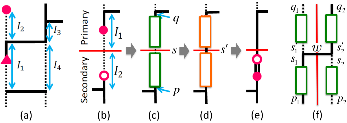
Suppose that a worm is on the th leg of the vertex. Here a leg is an interval delimited by the vertex in question on one end, and by another vertex or another worm on the other. Then, with probability , we let it enter the vertex, where is the length of the shortest of the four legs connected to the vertex [Fig. 1(a)]. Otherwise, we let it turn around without changing its position. If it enters the vertex, it chooses the out-going leg with probability , where is the weight of the state with the worm on the th leg. This is the usual scattering probability in DLA. Here, satisfies two equations, and , where runs over all leg indices. Finally, the imaginary time of the worm is chosen uniform randomly in the interval . These procedures define the following transition probability:
| (2) |
It is obvious that this transition probability satisfies the detailed-balance condition (to be more precise, the time-reversal symmetry condition in the present case), . The number of worm scatterings in a MC step is chosen so that every part of the space-time is updated roughly once on average.
Boundary-configuration update.—In the parallelized calculation, we decompose the whole space-time into multiple domains. Then, there are two special cases in the worm scattering discussed above; the case where the worm tries to enter a vertex connecting two domains (spatial domain boundary), and the case where the worm tries to go out of the current domain and enters another (temporal domain boundary). In these two cases, the worm is bounced by the vertex or the boundary with probability one. This treatment obviously satisfies the detailed-balance condition, but it breaks the ergodicity. In order to recover the ergodicity, we carry out the special update procedure described below in the region near the boundary at every MC step.
Figures 1(b)-(e) show the update procedure of a temporal boundary that has two “legs,” and [Fig. 1(b)], ending with states and , respectively. We choose the processor taking care of the upper domain as the “primary” and let it execute operations for updating the pair. The current local state just at the boundary is [Fig. 1(c)]. Then, the new state is chosen with the probability,
| (3) |
[Fig. 1(d)]. Once has been chosen, we can regenerate all worms in and with Eq. (1) as discussed previously [see Fig. 1(e)]. For hard-core bosons, for example, Eq. (3) is explicitly rewritten as , where and are the parities of and , respectively, and and .
The update procedure of the interdomain vertex is similar to that of the temporal boundary discussed above, although there are four intervals involved in this case instead of two. Suppose we have a vertex with four legs bounded with the ending states and below the vertex, and and above the vertex. Now, the new state variables at the roots of the four legs as shown in Fig. 1(f) are stochastically selected according to the product of the vertex weight and the leg weight ,
| (4) |
where is , previously referred to as in Eq. (2) with representing the set root states . Once the new root states have been selected, the rest of the task is the same as the temporal boundary update; i.e., we regenerate worms on the four legs. These tasks are carried out by the primary processor that takes care of the “left”-hand side of the vertex.
Pseudo code.—We summarize all of the procedure described above in the form of a pseudo code. The task of a processor in a MC step is as follows,
(Step 1) Send to and receive from the neighboring processor the ending states of the intervals on the temporal boundary. For each one of the intervals of which is primary, select the intermediate state stochastically with the probability Eq. (3). Send and receive the updated intermediate states.
(Step 2) Send to and receive from the neighboring processor the ending states of the legs of the vertices on the spatial boundary. For each one of the vertex of which is primary, select the states at the roots of the legs stochastically with the weight Eq. (4). Send and receive the updated root states.
(Step 3) As in the conventional DLA, erase all vertices without a kink on it, and place new vertices with the density proportional to the corresponding diagonal matrix element of the Hamiltonian.
(Step 4) For each interval delimited by the vertices or the domain boundaries, erase all the worms, generate an integer with the probability Eq. (1), generate a sequence of operators, and place them uniform randomly on . Also choose the direction of each worm with probability 1/2.
(Step 5) For every worm, if the nearest object ahead is a vertex that is not on a boundary, let it enter the vertex with the probability , let the worm scatter there with the probability , and choose the imaginary time uniform randomly on the final leg. Otherwise, reverse its direction without changing its position.
(Step 6) Repeat Step 5 more times, and perform measurements. This concludes the MC step.
Benchmark.—We apply the algorithm to the hard-core Bose-Hubbard model in the square lattice. The model we consider here is defined as
| (5) |
where is the chemical potential and denotes the nearest-neighbor interaction. In the PMWA, we simulate the Hamiltonian to generate multiple worms, then we extrapolate the QMC results to the limit. The extrapolation rule is given by the expansion of the physical quantity in a power series of where is small. For example, the coefficient of the first order term of the energy is as follows:
| (6) |
where is the mean value with respect to the nonperturbed Hamiltonian (5). When we choose to be a measure of the spontaneous symmetry breaking, as we do below, the right-hand side of Eq. (6) is always 0 for a finite system, making the term in vanish.
This result leads us to quadratic extrapolation , which shows good agreement with the conventional DLA result in the checkerboard solid (CS) phase [Fig. 2(a)]. In contrast, in the superfluid (SF) phase is finite in the thermodynamic limit at zero temperature. Even for finite systems at finite temperature, the deviation from the thermodynamic behavior at appears only in very small and practically not observed in large systems for which parallelization is necessary. It allows us to extrapolate the energy linearly at low temperatures as we see in Fig. 2(b) in which values are by the PMWA and by DLA. By closer inspection, however, we can also estimate the continuously varying scaling exponent, characteristic of the two-dimensional systems at finite temperature. Below we demonstrate that the present method can produce the off-diagonal order parameter, namely, the Bose-Einstein condensate (BEC) order parameter . The procedure for measuring this quantity and an arbitrary multipoint Green function, i.e. -sector measurements, is shown in the Supplemental Material [16]. Figure 2(c) shows the numerical results for systems ranging from to at fixed , which is much larger than a single processor can accommodate. We also present the result of extrapolation to the infinite limit for each value of based on the results of . The results calculated by using 3200 CPU cores agree well with the extrapolation. The dashed line is the power law fitting from which we can read the magnetization critical exponent .
It is in general possible that the domain boundaries hinder the propagation of the locally equilibrated region, and cause a slowing-down. In order to see the seriousness of this effect, we estimated the standard error, i.e., 1 standard deviation of the expected distribution, of the mean values of the order parameter and that of the energy in SF phase as a function of the number of domains in Fig. 3(a). We measured the quantities at every MC sweep, and the averages are taken over the same number of MC sweeps. Though the number of worms decrease with increasing , in all of our presented simulation the average number of worms in each domain is from to for used , and the probability of finding an empty domain is very low. We find a weak dependence of , which is empirically described as . We here emphasize that the PMWA is also efficient from the technical point of view; i.e., each processor has to communicate only with its neighbors, and the amount of transmitted information is proportional to the area of only the interface. This property is manifested in the good parallelization performance of our algorithm and code. For the so-called “weak scaling” performance, with the system size being proportional to the number of processors, see the Supplemental Material [16]. Figure 3(b) suggests good “strong scaling” performance, with the fixed system size and increasing number of processors. Specifically, it shows the standard error as a function of with both the system size and the elapsed time (“wall-clock” time) fixed. It plainly shows that we can achieve higher accuracy by employing more processors. The dependence of the error is described (again empirically) by which is slightly worse than the ideal dependence . The small difference in the exponent comes from the slight increase observed in Fig. 3(a).
We have presented a PMWA, a new parallelizable QMC algorithm, which can treat extremely large systems. We have applied it to hard-core bosons and observed high parallelization efficiency. The multibody correlation function should be computed relatively easily in the new algorithm. In addition, the PMWA can be extended in several ways. For example, “on-the-fly” vertex generation [17, 18], in which vertices are generated only in the immediate vicinity of the worms, is possible. Another extension may be the “wormless” algorithm. Obviously, the boundary update in terms of the parity of the number of worms rather than worms themselves can be used also for updating bulk regions. By doing so, we can altogether get rid of worms. These extensions will be discussed elsewhere [19]. The source code of our program will be released in Ref. [20] in the near future.
We would like to thank H. Matsuo, H. Watanabe, T. Okubo, R. Igarashi, and T. Sakashita for many helpful comments. This work was supported by CMSI/SPIRE, the HPCI System Research project (hp130007), and Grants-in-Aid for Scientific Research No. 25287097. Computations were performed on computers at the Information Technology Center of the University of the Tokyo, and at Supercomputer Center, ISSP.
.1 Supplemental Material
.2 S-I. Procedure of measuring the BEC order parameter and the multipoint Green function
We show here how to measure the BEC order parameter in our QMC method. The expectation value of an operator is expressed as follows,
where is the time-ordering operator. The numerator is
Thus, we obtain
The symbol denotes the MC observable for the density of worms at . It is defined as
where , the interval on which X is located, is split into and at . The final and initial states of are and respectively. Using , the MC observable of the arbitrary -body Green function is simply expressed as follows:
with the exceptions of the cases where multiple fall on the same interval. Details such as this will be discussed in our upcoming paper.
.3 S-II. Weak-scaling acceleration efficiency
The “weak scaling” acceleration efficiency is defined as , where is the elapsed computational time by using processors for a system with domains which have the fixed domain size as . When , the total size of a system with processors is , where . Figure 4 shows results of for hard-core Bose-Hubbard models (defined in our main text) in the square lattice. We tried various decomposition pairs with where , , , , , in Fig. 4(a) and (b), and , , in Fig. 4(c). In our calculation on FUJITSU PRIMEHPC FX10, we found that for large the efficiency is slightly less than 1. This slowing down may be caused by the “load balance” problem or by the information passing between processors. In all of our presented simulation, we confirmed that the amount of CPU time consumed by the information passing is negligibly small even when the number of processors is large (according to FUJITSU’s profiler data, of the total computational cost for the information passing and of the total computational cost for idle time when ). Therefore, the main source of the deviation from the ideal curve is the load-balancing, i.e., the amounts of computational tasks for processors become uneven causing some processors to finish their tasks earlier than the others and be idle. However, the efficiency only decreases by even when . The efficiency in a superfluid phase and a checkerboard solid phase turned out almost the same.
References
- [1] M. Suzuki, Prog. Theor. Phys. 56, 1454 (1976); M. Suzuki, S. Miyashita, and A. Kuroda, Prog. Theor. Phys. 58, 1377 (1977).
- [2] D. M. Ceperley, Rev. Mod. Phys. 67, 279 (1995).
- [3] P. Corboz, M. Boninsegni, L. Pollet, and M. Troyer, Phys. Rev. B 78, 245414 (2008).
- [4] F. D. M. Haldane, Phys. Rev. Lett. 50, 1153 (1983).
- [5] M. P. Nightingale and H. W. J. Blöte, Phys. Rev. B 33, 659 (1986).
- [6] K. Van Houcke, F. Werner, E. Kozik, N. Prokof’ev, B. Svistunov, M. J. H. Ku, A. T. Sommer, L. W. Cheuk, A. Schirotzek, and M. W. Zwierlein, Nat. Phys. 8 366 (2012).
- [7] H. G. Evertz, G. Lana, and M. Marcu, Phys. Rev. Lett. 70, 875 (1993).
- [8] N. Prokof’ev, B. Svistunov, and I. Tupitsyn, Sov. Phys. JETP 87, 310 (1998).
- [9] http://www.top500.org/.
- [10] B. Bauer, L. D. Carr, H. G. Evertz, A. Feiguin, J. Freire, S. Fuchs, L. Gamper, J. Gukelberger, E. Gull, S. Guertler, A. Hehn, R. Igarashi, S. V. Isakov, D. Koop, P. N. Ma, P. Mates, H. Matsuo, O. Parcollet, G. Pawłowski, J. D. Picon, L. Pollet, E. Santos, V. W. Scarola, U. Schollwöck, C. Silva, B. Surer, S. Todo, S. Trebst, M. Troyer, M. L. Wall, P. Werner, and S. Wessel, J. Stat. Mech. (2011) P05001.
- [11] K. Harada, T. Suzuki, T. Okubo, H. Matsuo, J. Lou, H. Watanabe, S. Todo, and N. Kawashima, Phys. Rev. B 88, 220408(R) (2013).
- [12] S. Trotzky, L. Pollet, F. Gerbier, U. Schnorrberger, I. Bloch, N. V. Prokof’ev, B. Svistunov, and M. Troyer, Nat. Phys. 6, 998 (2010).
- [13] O. F. Syljuåsen and A. W. Sandvik, Phys. Rev. E 66, 046701 (2002).
- [14] N. Kawashima and K. Harada, J. Phys. Soc. Jpn. 73, 1379 (2004).
- [15] A. Dorneich and M. Troyer: Phys. Rev. E 64 066701 (2001).
- [16] See Supplemental Material for the procedure of measuring the BEC order parameter and the multipoint Green function, and for the acceleration efficiency for weak scaling of PMWA.
- [17] Y. Kato, T. Suzuk, and N. Kawashima, Phys. Rev. E 75, 066703 (2007).
- [18] L. Pollet, K. V. Houcke, and S. M. A. Rombouts J. Comp. Phys. 225, 2249 (2007).
- [19] A. Masaki-Kato, T. Suzuki, K. Harada, S. Todo, and N. Kawashima, to be published.
- [20] http://ma.cms-initiative.jp/en/application-list/dsqss/dsqss