Efficient linear-scaling quantum transport calculations on graphics processing units and applications on electron transport in graphene

Based on the discussion of the last section, we see that the quantities that need to be calculated are $\rho(E)$, $\rho(E)C_{vv}(E,t)$, and $\rho(E)\Delta X^{2}(E,t)$. To facilitate the numerical calculation, we firstly rewrite $\rho(E)C_{vv}(E,t)$ and $\rho(E)\Delta X^{2}(E,t)$ in the following symmetric forms (using the cyclic properties of the trace):

The reason for this will be apparent when we consider the GPU-implementation. To achieve linear-scaling, we have to make three approximations presented below.

In this subsection, we consider the GPU implementation of the algorithms. We use CUDA [38] as our developing tool. We only discuss the relevant techniques of our CUDA implementation when appropriate; the reader is referred to the official programming guide [38] for more details.

To achieve high performance, we implement nearly all of the algorithms on the GPU, minimizing data transfer between the CPU and the GPU. Here we present the pseudo codes for calculating $\rho(E)$, $\rho(E)C_{vv}(E,t)$, and $\rho(E)\Delta X^{2}(E,t)$ in Algorithms 1, 2, and 3, respectively. While for $\rho(E)$, we only need to calculate one set of moments, for $\rho(E)C_{vv}(E,t)$ and $\rho(E)\Delta X^{2}(E,t)$, we have to calculate a set of moments at each correlation time $t_{m}$ $(0\leq m<N_{c})$. Thus, calculating the conductivity is generally much more demanding than calculating the DOS. Note that we only calculate the moments in the GPU, and copy their results to the CPU for performing the Fourier transform or the Chebyshev summation. We could do all the calculations in the GPU, but it does not result in a significant gain in the overall performance, since the calculation of the moments takes the majority of the computation time.

In the previous subsection, we have written $\rho(E)C_{vv}(E,t)$ and $\rho(E)\Delta X^{2}(E,t)$ in symmetric forms. The advantage is that we can use the following iteration relations to calculate the conductivity at different correlation times:

The calculation of the moments in both the FTM and the KPM used in the above three algorithms can also be carried out iteratively. We note that the Fourier moments in equations (25 - 27) can be expressed in a unified way:

Different moments only differ in $|\phi_{L}\rangle$ and $|\phi_{R}\rangle$: for DOS, $|\phi_{L}\rangle=|\phi_{R}\rangle=|\phi\rangle$; for VAC, $|\phi_{L}\rangle=VU^{\dagger}(t)|\phi\rangle$ and $|\phi_{R}\rangle=U^{\dagger}(t)V|\phi\rangle$; for MSD, $|\phi_{L}\rangle=|\phi_{R}\rangle=[X,U(t)]|\phi\rangle$. Similarly, the Chebyshev moments in equations (32 - 34) can be expressed uniformly as

Thus, we can present the calculations of these different moments in a unified way, as shown in Algorithms 4 and 5.

We next consider the time-evolution of quantum states. In Algorithms 6 and 7, we present the algorithms for evaluating $|\phi_{\textmd{out}}\rangle=U(\pm\Delta t)|\phi_{\textmd{in}}\rangle$ and $|\phi_{\textmd{out}}\rangle=[X,U(\Delta t)]|\phi_{\textmd{in}}\rangle$, according to Eq. (36) and Eq. (37), respectively. In Algorithm 6, besides the input vector $|\phi_{\textmd{in}}\rangle$, and the output vector $|\phi_{\textmd{out}}\rangle$, we need three auxiliary vectors, $|\phi_{0}\rangle$, $|\phi_{1}\rangle$, and $|\phi_{2}\rangle$. In Algorithm 7, we need another set of auxiliary vectors, $|\phi_{0}^{x}\rangle$, $|\phi_{1}^{x}\rangle$, and $|\phi_{2}^{x}\rangle$. All of these vectors should be defined in global memory in order to pass data between kernels.

An examination of Algorithms 6 and 7 reveals that, apart from some simple linear transformations, the only nontrivial calculations are the matrix-vector multiplications, $|\phi_{\textmd{out}}\rangle=H|\phi_{\textmd{in}}\rangle$ and $|\phi_{\textmd{out}}\rangle=[X,H]|\phi_{\textmd{in}}\rangle$. In Algorithm 8, we present the pseudo code of the CUDA kernel which evaluates $|\phi_{\textmd{out}}\rangle=H|\phi_{\textmd{in}}\rangle$; the evaluation of $|\phi_{\textmd{out}}\rangle=[X,H]|\phi_{\textmd{in}}\rangle$ is very similar.

The strategy in Algorithm 8 is to use one thread for one element of the output vector. By using a block size of $S_{b}$, the number of blocks in the kernel is $(N-1)/S_{b}+1$, where $N$ is the number of sites in the system. Thus, this kernel is executed with the configuration of $<<<(N-1)/S_{b}+1,S_{b}>>>$. The if statement on line 1 is necessary to avoid manipulating invalid memory in the case of $N$ not being an integer multiple of $S_{b}$. Lines 2-7 are devoted to the calculation of $\phi_{\textmd{out}}[n]$, where the variable temp is used to reduce the global memory access, which is very time-consuming. We use a neighbor list to specify the Hamiltonian, denoting the number of neighbors to site $n$ as NN_n, and indexing the $k$th neighbor of site $n$ as NL_nk. For a sparse Hamiltonian, NN_n is much smaller than the total number of sites $N$. The NL_nk data should be coded in such a way that the indices of the $k$th neighbor sites for all the sites are stored consecutively, i.e., in the order of NL₀₀, NL₁₀, NL₂₀, $\cdots$, NL₀₁, NL₁₁, NL₂₁, $\cdots$, NL_0k, NL_1k, NL_2k, $\cdots$. This special order ensures coalescing in global memory access, which means that consecutive threads access consecutive data in the global memory. This requirement has also been noticed in our previous work on molecular dynamics simulations [39].

We firstly evaluate the relative performance of our GPU implementation with respect to our CPU implementation. The comparison is made between a Tesla K20 GPU card and an Intel Xeon E5-1620 @ 3.60 GHz CPU core. The serial CPU code is implemented in C/C++ and is compiled with an O3 optimization mode. Although the algorithms in the previous section are presented by using a complex number notation, in both the CPU and the GPU implementation, we use two real vectors for a complex state vector, which can save nearly half of the calculations compared with a naive use of the intrinsic complex number. Both the CPU and the GPU code use double-precision arithmetics.

The major computation which scales linearly with the system size is the Chebyshev iteration, which is used for both the time-evolution and the KPM. We thus present a performance evaluation of the Chebyshev iteration part of the code in some detail. We chose to present the testing results for $|\phi_{2}\rangle=2H|\phi_{1}\rangle-|\phi_{0}\rangle$; those for $|\phi_{2}^{x}\rangle=2[X,H]|\phi_{1}\rangle+2H|\phi_{1}^{x}\rangle-|\phi_{0}^{x}\rangle$ are similar.

Figure 1 shows the results of the performance evaluation of the Chebyshev iteration part, where the speedup factor is defined as the computation time in the CPU over that in the GPU. The computational time in the CPU scales linearly with respect to the simulation size, which reflects the linear-scaling nature of the algorithm. The computation time in the GPU also scales linearly approximately. The speedup factor increases from about 10.5 to about 16.5 with the number of atoms in the simulated system increasing from 0.2 million to 1.6 million and nearly saturates thereafter. For all the other calculations such as the evaluation of the inner products, we also obtained a comparable speedup factor. The overall speedup factor of our GPU implementation over our CPU implementation is observed to be about 16.

This speedup factor seems to be not very impressive. Indeed, in our recent work on exact diagonalization of the Hubbard model using the LRM on the GPU [40], a speedup factor of about 60 is obtained using double-precision. The difference in the speedup factor results from the different computational intensities of the problems. For example, in the Hubbard model, for a Hamiltonian size of 853776 (12 spin sites), the computation times for one Lanczos iteration in the CPU and the GPU are about 120 ms and 2 ms, respectively, giving a speedup factor of 60 [40]. In comparison, for our tight-biding model with a Hamiltonian size of $10^{6}$, the computation times for one Chebyshev iteration in the CPU and the GPU are about 12.8 ms and 0.8 ms, giving a speedup factor of 16. We see that for a given Hamiltonian size, the Hubbard model is about 10 times more computationally intensive than the single-particle tight-binding model and attains a higher speedup factor. Similar dependence of the speedup factor on the computational intensity has also been observed in our recent work on molecular dynamics simulation [39].

We then give a comparison of the relative performance of the KPM and the FTM. For the FTM, the calculation of each Fourier moment involves a time-evolution with a time step $\Delta\tau$. The choice of the time step used in the FTM is related to the Nyquist sampling rates used in digital signal analysis: it should not be too large to give aliasing errors, and not too small to reduce the energy resolution [31]. The optimal value of $\Delta\tau$ corresponding to a maximum bandwidth $\Delta E$ of the energy spectrum without aliasing error can be fixed to be

For a scaled Hamiltonian with spectrum $[-1,1]$, we have $\Delta E=2$ and $\Delta\tau=\pi\hbar$. Then, the dimensionless argument in the Bessel function is $\pi$, which determines the number of Chebyshev iterations in the time evolution operator $U(\Delta\tau)$ to be about $N_{p}=20$ for an accuracy of $10^{-15}$. In contrast, the calculation of each Chebyshev moment in the KPM only involves one Chebyshev iteration.

To give a fair comparison of the relative efficiency, we should also consider the energy resolution $\delta E$, which is related to the number of moments $2N_{m}+1$ in the FTM and $N_{m}$ in the KPM. Quantitatively, we have

in the FTM [31] and

in the KPM [28], respectively. Figure 2 gives a comparison of the DOSs calculated by the the KPM with $N_{m}=1000$ and the FTM with $2N_{m}+1=1001$. We see that they give consistent results and the FTM indeed has a higher energy resolution when using the same number of moments.

By combining the above analysis, we come to the conclusion that the KPM is about $20/\pi\approx 6.4$ times as efficient as the FTM for achieving the same energy resolution. However, for the transport simulations, this difference of efficiency only matters in the diffusive regime, where the correlation time step $\Delta t$ should be relatively small, and the computation time is dominated by the calculation of the $\delta$ function. In the localized regime, where the correlation time step is usually chosen to be very large, the computation time is dominated by the time-evolution $[X,U(t)]|\phi\rangle$, and the relative efficiency of the KPM over the FTM does not lead to a significant gain in performance for the whole simulation.

For ballistic transport without any scattering, the VAC does not decay with time, resulting in a divergent conductivity. A finite conductance can only be deduced by introducing a length scale. While there is no intrinsic definition of length in the Green-Kubo and the Einstein formulas, a definition of length in terms of the MSD,

is frequently used [10, 17, 18]. The conductance of a system with width $W$ can be defined as

Although the correlation time $t$ appears in the above equation, a converged time-independent (length-independent) value of $G(E)$ can be obtained within a short correlation time. We note that the factor of 2 in the above length definition is necessary to obtain correct results if we use the correct definition of conductivity, $\sigma^{\textmd{E1}}(E,t)$, rather than the alternative, $\sigma^{\textmd{E2}}(E,t)$, which is half of $\sigma^{\textmd{E1}}(E,t)$ in the ballistic regime.

To justify the factor of 2 in Eq. (50), we examine the time-dependence of the length for pristine graphene with different sizes and different boundary conditions along the transport direction, which is chosen to be the zigzag direction. By applying periodic boundary conditions in the transport direction, there is no noticeable difference in the results obtained by using a longer sample (252 nm for $2048\times 1024$ graphene) and a shorter sample (126 nm for $1024\times 1024$ graphene), which reflects the small finite size effect in Green-Kubo-like formulas [39]. In contrast, by imposing a non-periodic boundary condition in the transport direction, the diffusion of electrons is confined by the sample size, with the maximum diffusion length as defined in Eq. (50) being the length of the sample. The factor of 2 can also be understood intuitively: $\sqrt{\Delta X^{2}(E,t)}$ is the absolute diffusion distance in one direction, and the factor of 2 accounts for the diffusion in the opposite direction.

We now study the ballistic transport properties of a $65536\times 16$ pure ZGNR by comparing the results with those obtained by the NEGF method. As can be seen from Fig. 4 (a), the overall plateaus of the quantized conductance can be correctly produced by Eq. (51), but the conductances around the band edges are overestimated. Markussen et al. [12] also noticed this problem and argued that the overshoots near the band edges originate from the nonequivalence between the expectation values of $v(E)$ and the square root of the expectation value of $v^{2}(E)$. Here, we give an analysis of this problem from the numerical perspective.

In the ballistic regime, the VAC oscillates around some value (see Fig. 4 (d) for an example), and an average value of $v^{2}(E)$ can be well established over a short correlation time. Thus we can express the MSD as $\Delta X^{2}(E,t)=v^{2}(E)t^{2}$, which results in the following expression for the conductance:

Fig. 4 (b) presents the calculated DOS and Fig. 4 (c) presents the deduced $\sqrt{v^{2}(E)}$. We see that both $\rho(E)$ and $\sqrt{v^{2}(E)}$ are singular near the band edges. Thus, the calculation of ballistic conductance in the Einstein formalism involves multiplications of big and small numbers, which is numerically unstable. Since the MSD and the VAC are squared quantities, we obtain an overestimation rather than an underestimation of the conductance.

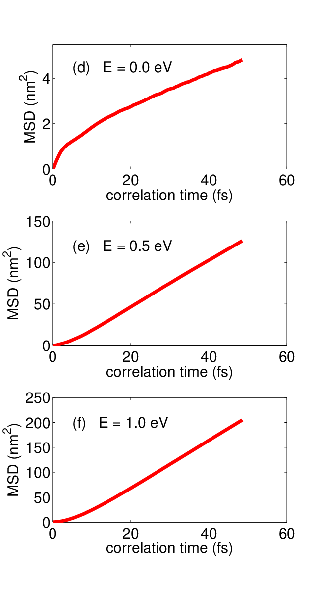
We now turn to discuss the diffusive transport regime. We consider 2D graphene of size $2048\times 1024$ with defect concentration $n=1\%$. We use both the Green-Kubo formula and the Einstein formula. The time step is chosen to be $\Delta t=0.1$ fs, small enough to exhibit the detailed features of the ballistic-to-diffusive transition.

Figure 5 (a-c) shows the VACs for different energies as a function of correlation time. We see that the VAC does not decay monotonically. For the Dirac point $E=0.0$ eV, the VAC decays to zero within one fs and then develops negative values up to 5 fs, after which the VAC stays at zero for a relatively long time. For higher energies, $E=0.5$ eV and 1.0 eV, apart from the expected exponential decay, there is also an oscillatory component. This oscillation has been discussed by de Laissardiere el al. [16], and is attributed to the Zitterbewegung effect. A spectral analysis shows that the frequency $\omega$ of the oscillation is directly related to the electron energy by $\omega=2E/\hbar$, which is consistent with the oscillation factor $\cos^{2}(Et/\hbar)$ in the VAC [16]. By going from the Green-Kubo to the Einstein formalism, these oscillations are smoothed out, as shown by the MSD curves in Figure 5 (d-f). The ballistic-to-diffusive transition is featured by the decay of the VAC in the Green-Kubo formalism, or the quadratic-to-linear transition of the MSD in the Einstein formalism.

From the VAC and the MSD, we can calculate RECs, $\sigma^{\textmd{GK}}(E,t)$, $\sigma^{\textmd{E1}}(E,t)$, and $\sigma^{\textmd{E2}}(E,t)$, as shown in Fig. 5 (g-i). We see that the derivative-based definition of the REC in the Einstein formalism is equivalent to the REC defined in the Green-Kubo formalism: $\sigma^{\textmd{E1}}(E,t)=\sigma^{\textmd{GK}}(E,t)$. In contrast, the division-based definition of the REC in the Einstein formalism deviates from the other two in the ballistic-to-diffusive regime. One may note that for the Dirac point, $\sigma^{\textmd{E1}}(E,t)$ has large fluctuations when $t>10$ fs. This reflects the numerical difficulty of calculating the derivative in Eq. (9), especially for small time steps, and is probably the reason for the preference of using $\sigma^{\textmd{E2}}(E,t)$ instead of $\sigma^{\textmd{E1}}(E,t)$ in some previous works. However, we stress that $\sigma^{\textmd{E2}}(E,t)$ is a wrong definition in principle and should be used with caution.

The most interesting quantity in the diffusive regime is the semi-classical conductivity, $\sigma_{\textmd{sc}}$, which is conventionally defined [11, 12, 13, 14, 15, 16, 17, 19, 18, 20, 21] to be the maximum value of the REC:

Using this definition, the calculated $\sigma_{\textmd{sc}}(E)$ (the solid line in Fig. 6) exhibits a plateau of minimum conductivity $\sigma_{\textmd{min}}=4e^{2}/(\pi h)$ in the range of $|E|<$ 0.25 eV, along with a peak around the Dirac point. Similar results have been obtained by Yuan et al. using the Green-Kubo formula [23] and by Cresti et al. using the Einstein formula [21]. One may note that the peaks found by Yuan et al. [23] are much lower than those found by Cresti et al. [21]. This difference partly results from the different numerical approaches, but the major reason is that Cresti et al. use Eq. (53) to calculate $\sigma_{\textmd{sc}}(E)$, while Yuan et al. just integrate the VAC to some given correlation time.

A comment on the connection and difference between the Green-Kubo method in our work and the numerical approach developed by Yuan et al. is in order. After some algebra, we can rewrite their formula for DC conductivity (Eq. (41) in Ref. [23]) using our notations as:

which is equivalent to Eq. (6) and Eq. (20) in our work. The difference between our approach and their is mainly related to the numerical implementations. They firstly precompute all the “quasi-eigenstates” $|E_{m}\rangle=\delta(E_{m}-H)|\phi\rangle\approx\frac{\Delta\tau}{2\pi\hbar}\sum_{n=-N_{m}}^{+N_{m}}e^{iE_{m}n\Delta\tau/\hbar}U(n\Delta\tau)|\phi\rangle$ for a given number of energy points $E_{m}$ and then store them in memory, before calculating $\sigma(E,t)$ using Eq. (54). This strategy may be very efficient, but is not economic in terms of memory usage, restricting the number of energy points considered in one simulation to be around 64 [24].

References

- [1] S. Datta, Electonic Transport in Mesoscopic Systems. Cambridge University Press, 1995.
- [2] R. Kubo, Statistical-Mechanical Theory of Irreversible Processes. I. General Theory and Simple Applications to Magnetic and Conduction Problems, J. Phys. Soc. Jpn. 12, (1957) 570-586.
- [3] D. A. Greenwood, The Boltzmann Equation in the Theory of Electrical Conduction in Metals. Proc. Phys. Soc. 71, (1958) 585-596.
- [4] A. K. Geim and K. S. Novoselov, The rise of graphene, Nature Materials, 6, (2007) 183-191.
- [5] A. H. Castro Neto, F. Guinea, N. M. R. Peres, K. S. Novoselov and A. K. Geim, The electronic properties of graphene, Rev. Mod. Phys., 81, (2009) 109-162.
- [6] M. P. L. Sancho, J. M. L. Sancho and J. Rubio, Highly convergent schemes for the calculation of bulk and surface Green functions, J. Phys. F: Met. Phys, 15 (1985) 851-858.
- [7] D. Mayou, Calculation of the Conductivity in the Short-Mean-Free-Path Regime, Europhys. Lett. 6, (1988) 549-554.
- [8] D. Mayou and S. N. Khanna, A Real-Space Approach to Electronic Transport, J. Phys. I Paris 5, (1995) 1199-1211.
- [9] S. Roche and D. Mayou, Conductivity of quasiperiodic systems: a numerical study, Phys. Rev. Lett. 79, (1997) 2518-2521.
- [10] F. Triozon, J. Vidal, R. Mosseri, and D. Mayou, Quantum dynamics in two- and three-dimensional quasiperiodic tilings, Phys. Rev. B 65, (2002) 220202(R).
- [11] F. Triozon, S. Roche, A. Rubio, and D. Mayou, Electrical transport in carbon nanotubes: Role of disorder and helical symmetries, Phys. Rev. B 69, (2004) 121410(R).
- [12] T. Markussen, R. Rurali, M. Brandbyge, and A.-P. Jauho, Electronic transport through Si nanowires: Role of bulk and surface disorder, Phys. Rev. B 74 (2006) 245313.
- [13] H. Ishii, N. Kobayashi, and K. Hirose, Order- electron transport calculations from ballistic to diffusive regimes by a time-dependent wave-packet diffusion method: Application to transport properties of carbon nanotubes, Phys. Rev. B 82, (2010) 085435.
- [14] A. Lherbier, B. Biel, Y.-M. Niquet, and S. Roche, Transport Length Scales in Disordered Graphene-based Materials: Strong Localization Regimes and Dimensionality Effects, Phys. Rev. Lett. 100, (2008) 036803.
- [15] A. Lherbier, X. Blase, Y.-M. Niquet, F. Triozon and S. Roche, Charge Transport in Chemically Doped Graphene, Phys. Rev. Lett. 101, (2008) 036808.
- [16] G. T. de Laissardiere and D. Mayou, Electronic transport in graphene: quantum effects and role of local defects, Modern Physics Letters B, 25 (2011) 1019-1028.
- [17] N. Leconte, A. Lherbier, F. Varchon, P. Ordejon, S. Roche, and J.-C. Charlier, Quantum transport in chemically modified two-dimensional graphene: From minimal conductivity to Anderson localization, Phys. Rev. B 84 (2011) 235420.
- [18] A. Lherbier, S. M.-M. Dubois, X. Declerck, Y.-M. Niquet, S. Roche, and J.-C. Charlier, Transport properties of graphene containing structural defects, Phys. Rev. B. 86, (2012) 075402.
- [19] T. M. Radchenko, A. A. Shylau, and I. V. Zozoulenko, Influence of correlated impurities on conductivity of graphene sheets: Time-dependent real-space Kubo approach, Phys. Rev. B 86, (2012) 035418.
- [20] D. Van Tuan, J. Kotakoski, T. Louvet, F. Ortmann, J. C. Meyer, and S. Roche, Scaling properties of charge transport in polycrystalline graphene, Nano Lett. 13, (2013) 1730-1735.
- [21] A. Cresti, F. Ortmann, T. Louvet, D. Van Tuan, and S. Roche, Broken symmetries, zero-energy modes, and quantum transport in disordered graphene: from supermetallic to insulating regimes, Phys. Rev. Lett. 110, (2013) 196601.
- [22] W. Li, H. Sevinçli, S. Roche, and G. Cuniberti, Efficient linear scaling method for computing the thermal conductivity of disodered materials, Phys. Rev. B 83, (2011) 155416.
- [23] S. Yuan, H. De Raedt, and M. I. Katsnelson, Modeling electronic structure and transport properties of graphene with resonant scattering centers, Phys. Rev. B. 82, (2010) 115448.
- [24] S. Yuan, H. De Raedt, and M. I. Katsnelson, Electronic transport in disordered bilayer and trilayer graphene, Phys. Rev. B. 82, (2010) 235409.
- [25] S. Yuan, R. Roldán, A.-P. Jauho, and M. I. Katsnelson, Electronic properties of disordered graphene anditod lattices, Phys. Rev. B. 87, (2013) 085430.
- [26] A. Harju, T. Siro, F. Federici-Canova, S. Hakala, and T. Rantalaiho, Computational Physics on Graphics Processing Units, Lecture Notes in Computer Science, 7782, (2013) 3-26.
- [27] M. S. Green, Markoff Random Processes and the Statistical Mechanics of Time-Dependent Phenomena. II. Irreversible Processes in Fluids, J. Chem. Phys. 22 (1954) 398-413.
- [28] A. Weiße, G. Wellein, A. Alvermann, and H. Fehske, The kernel polynomial method, Review of Modern Physics. 78, (2006) 275-306.
- [29] R. Haydock, V. Heine and M. J Kelly, Electronic structure based on the local atomic environment for tight-binding bands, J. Phys. C: Solid State Phys. 5, (1972) 2845-2858.
- [30] R. Haydock, V. Heine and M. J Kelly, Electronic structure based on the local atomic environment for tight-binding bands. II, J. Phys. C: Solid State Phys. 8, (1975) 2591-2605.
- [31] M. D. Feit, J. A. Fleck, Jr., and A. Steiger, Solution of the Schrödinger Equation by a Spectral Method, Journal of Computational Physics, 47, (1982) 412-433.
- [32] A. Hams and H. De Raedt, Fast algorithm for finding the eigenvalue distribution of very large matrices, Phys. Rev. E. 62, (2000) 4365-4377.
- [33] H. Tal-Ezer and R. Kosloff, An Accurate and Efficient Scheme for Propagating the Time Dependent Schrödinger Equation, J. Chem. Phys. 81, (1984) 3967-3971.
- [34] H. Fehske, J. Schleede, G. Schubert, G. Wellein, V. S. Filinov, and A. R. Bishop, Numerical approaches to time evolution of complex quantum systems, Physics Letters A 373, (2009) 2182-2188.
- [35] T. Dziubak and J. Matulewski, An object-oriented implementation of a solver of the time-dependent Schrödinger equation using the CUDA technology, Computer Physics Communications, 183 (2012) 800-812.
- [36] C. Ó Broin, and L. A. A. Nikolopoulos, An OpenCL implementation for the solution of the time-dependent Schrödinger equation on GPUs and CPUs, Computer Physics Communications, 183, (2012) 2071–2080.
- [37] T. Siro and A. Harju, Time Propagation of Many-Body Quantum States on Graphics Processing Units, Lecture Notes in Computer Science, 7782, (2013) 141-152.
- [38] NVIDIA, CUDA Programming Guide, version 5.0 (2013).
- [39] Z. Fan, T. Siro, and A. Harju, Accelerated molecular dynamics force evaluation on graphics processing units for thermal conductivity calculations, Computer Physics Communications, 184, (2013) 1414-1425.
- [40] T. Siro, A. Harju, Exact diagonalization of the Hubbard model on graphics processing units, Computer Physics Communications, 183 (2012) 1884-1889.
- [41] P. K. Schelling, S. R. Phillpot, and P. Keblinski, Comparison of atomic-level simulation methods for computing thermal conductivity, Phys. Rev. B 65 (2002) 144306.
- [42] A. Ferreira, J. Viana-Gomes, J. Nilsson, E. R. Mucciolo, N. M. R. Peres, and A. H. Castro Neto, Unified description of the dc conductivity of monolayer and bilayer graphene at finite densities based on resonant scatterers, Phys. Rev. B 83, (2011) 165402.
- [43] Private communication with A. Ferreira.
- [44] P. W. Anderson, D. J. Thouless, E. Abrahams, and D. S. Fisher New method for a scaling theory of localization Phys. Rev. B 22, (1980) 3519.
- [45] A. Uppstu, K. Saloriutta, A. Harju, M. Puska, and A.-P. Jauho, Electronic transport in graphene-based structures: An effective cross-section approach Phys. Rev. B 85, (2012) 041401(R).
- [46] D. S. Fisher and P. A. Lee, Relation between conductivity and transmission matrix, Phys. Rev. B 23, (1981) 6851-6854.
- [47] J. A. Vergés, Computational implementation of the Kubo formula for the static conductance: application to two-dimensional quantum dots, Computer Physics Communications, 118, (1999) 71-80.
- [48] B. K. Nikolić, Deconstructing Kubo formula usage: Exact conductance of a mesoscopic system from weak to strong disorder, Phys. Rev. B 64, (2001) 165303.
- [49] G. Schubert, J. Schleede, and H. Fehske, Anderson disorder in graphene nanoribbons: A local distribution approach, Phys. Rev. B 79, (2009) 235116.