Effective Josephson dynamics in resonantly driven Bose-Einstein condensates
Abstract
We show that the orbital Josephson effect appears in a wide range of driven atomic Bose-Einstein condensed systems, including quantum ratchets, double wells and box potentials. We use three separate numerical methods: Gross-Pitaevskii equation, exact diagonalization of the few-mode problem, and the Multi-Configurational Time-Dependent Hartree for Bosons algorithm. We establish the limits of mean-field and few-mode descriptions, demonstrating that they represent the full many-body dynamics to high accuracy in the weak driving limit. Among other quantum measures, we compute the instantaneous particle current and the occupation of natural orbitals. We explore four separate dynamical regimes, the Rabi limit, chaos, the critical point, and self-trapping; a favorable comparison is found even in the regimes of dynamical instabilities or macroscopic quantum self-trapping. Finally, we present an extension of the -formalism to general time-periodic equations of motion, which permits a systematic description of the long-time dynamics of resonantly driven many-body systems, including those relevant to the orbital Josephson effect.
pacs
03.75.Lm,67.85.De,67.10.JnI Introduction
In a bosonic Josephson junction (BJJ) two or a few single-particle states are coherently occupied by a macroscopic number of bosons [1]. These systems combine two qualities that make them interesting for experimental and theoretical studies. First, they are a quantum many-body system. Second, the underlying Hilbert space grows only linearly with the total particle number for the case of two single-particle states. Thus BJJs provide a simple framework to study the role of particle interactions in quantum gases. Due to the possibility of conveniently controlling the classical limit via the particle number, these systems are particularly well suited for the study of some aspects of the quantum-classical crossover [2, 3, 4].
The Josephson effect in Bose-Einstein condensates (BECs) can exist in a variety of qualitatively different forms. In an external Josephson junction [5], the modes involved refer to localized Wannier functions in a double-well potential. A more robust realization is provided by the so-called internal Josephson effect [6, 7], where the states are defined by the different electronic configurations of the gas atoms. Dissipation due to the exchange of non-condensed atoms leads to Ohmic damping of the Josephson oscillations [8]. Bosonic Josephson junctions can also be used for high precision measurement of physical quantities such as temperature [9], weak forces (gravitational [10] or electroweak [11]), or chemical potential differences [12]. Promising scenarios for the creation of macroscopic superposition states [13] or spin-squeezed states [14] are based on BJJs. Furthermore, in a recent experiment at NIST [15], a BJJ in an atom circuit was used to measure rotation.

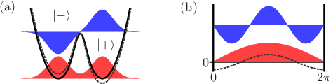
Recently, a third kind of Josephson effect in BECs, not classifiable as external or internal, has been identified. In the orbital Josephson effect (OJE) the single-particle modes have identical internal structure and center-of-mass wave functions with strongly overlapping densities (see Fig. 1). The OJE can be realized when a time-periodic driving potential induces a coupling among the unperturbed Floquet states of the system. Previous work on the OJE [16] has focused on the quantum ratchet on a ring potential because the OJE was originally identified in that context. This kind of system is realizable in current BEC setups. In fact an orbital Josephson junction can be obtained in a variety of static and driving potentials. The present work aims at presenting the OJE in a very general context. Starting with two very simple illustrative examples, a double well [5] and a box potential [17], we show that the OJE is a general concept that can be studied in a variety of existing experimental BEC systems. Then we explore different driving potentials in ring traps, inspired by recent experimental successes [18, 19, 20, 21, 22, 23, 24, 15].
For some selected cases, our theoretical model based on an effective few-mode Hamiltonian is compared to computationally demanding simulations from first principles performed with the Multi-Configurational Time-Dependent Hartree for Bosons (MCTDHB) algorithm [25, 26, 27]. For the present purposes, MCTDHB can be regarded as a method that enables a full many-body (FMB) study of the interacting boson problem. Thus we focus on the comparison between the truncated description of the orbital Josephson effect and a full many-body calculation that operates in a larger one-atom Hilbert space. Importantly, in both these pictures we work well-beyond the Gross-Pitaevskii (GP) approximation [28, 29], which is also considered in some cases. We find that the MCTDHB results agree well with the truncated BJJ description in a variety of dynamical regimes. This includes regimes that show instabilities in the semiclassical limit such as chaos and unstable fixed points which are poorly described within the GP approximation. Interestingly, we find that the regime of macroscopic quantum self-trapping preserves its character in a non-truncated, full many-body description. This contrasts with the case of an undriven double-well potential (external Josephson effect), where self-trapping seems to be fragile within a multi-mode picture [30].
A major contribution of this paper is the generalization of the so-called -formalism [31, 32] to an almost arbitrary type of equation of motion including the nonlinear Schrödinger equation. The -formalism has shown to be an efficient mathematical tool for the study of time-periodic [32, 33] and aperiodic [34] linear systems. Here we employ the extended -formalism to analyze the dynamics of field operators in interacting many-body systems.
This paper is arranged as follows. Section II presents general two-mode orbital Josephson junctions, without specification of the trap geometry or the driving potential. It also includes a rather general presentation of the -formalism for field operators. Section III introduces two illustrative examples of the orbital Josephson effect: a rocked double well and a box potential perturbed with a modulated lattice. In Section IV the previously introduced concepts are used to explore in greater depth the case of a BEC in a ring trap subject to a ratchet potential. Up to three different driving potentials are discussed, each yielding a three-mode orbital Josephson system. Finally in Section V, we compare the predictions from the effective description in terms of an orbital Josephson junction with full many-body simulations using MCTDHB, focusing on one of the driving potentials introduced in Section IV. In Appendix A the extended -formalism is derived in great generality. Appendix B addresses technical details of the numerical MCTDHB study.
II General concepts
In this section, we present a recipe for the realization of an orbital Josephson junction. We will keep our approach as general as possible. However, in Section IV, we will see that a variety of orbital Josephson junctions also exist which cannot be considered a specific realization of the type presented here.
We consider an initially static BEC, trapped in an arbitrary geometry, given by some static external potential . At time , a time-periodic driving potential with periodicity ,
| (1) |
is switched on. The dynamics of this many-body system is determined by the Heisenberg equation of motion for bosonic field operators,
| (2) |
where time and spatial coordinates are made dimensionless. This can be realized by the choice of an appropriate length scale and then expressing all lengths, energies, frequencies, and times in units of , , , and , respectively, where is the atom mass. Furthermore, we set , such that energies and frequencies have the same dimensions. The single-particle Hamiltonian is a sum of kinetic energy and external potential. The initial field operator annihilates a bosonic particle at point and satisfies the standard bosonic commutation relations and , which are preserved in time. The contact interaction strength is proportional to the s-wave scattering length of the gas atoms.
Our goal is to develop an effectively time-independent description that involves only two single-particle states. We do this by using an extended version of the -formalism to describe the dynamics of the field operators in second quantization [16]. The -formalism has proven to be a powerful tool for solving the Schrödinger equation with time-dependent Hamiltonians [31, 32]. The equation of motion for the field operators (2) reads in the extended -formalism
| (3) |
where acts as an additional parameter which the field operators depend on. The single-particle part is the sum of kinetic energy, trapping potential, and a driving potential. Equation (3), together with the initial conditions,
| (4) |
define a unique solution for , from which the physically relevant field operator can be obtained via
| (5) |
Note that, the periodicity in , which is trivially imposed by the initial condition, Eq. (4), holds for all times, since the equation of motion (3) does not break this symmetry. Furthermore, under these initial conditions the initial commutation relations are also preserved, which read
| (6) |
We assume the static single particle part to be the predominant term in the equation of motion (2). This condition is met for systems with weak particle interactions , and a weak overall amplitude of the driving potential . Furthermore, this assumptions implies, that the low energy eigenstates of the undriven () system are condensates, with a negligible amount of depletion [35] and with the condensate orbitals given by eigenstates of .
Within the -formalism, this means that the predominant part is given by the unperturbed single-particle Floquet operator
| (7) |
suggesting one ought to use a transformed representation of Eq. (3) that involves creation and annihilation operators with respect to the unperturbed Floquet states (eigenmodes of ).
II.1 Floquet representation in second-quantized form
Therefore, we introduce the representation given by
| (8) |
where denotes an eigenmode of . The corresponding unperturbed single-particle quasienergy is given by , where is the energy of . Quasienergies can be considered the time analog to quasi-momentum from Bloch theory. The inverse transformation to Eq. (8) reads
| (9) |
where the sum over runs over all integer numbers and indicates the eigenstates . In this representation, the commutation relations (6) become
| (10) | ||||
| (11) |
In order to obtain an equation of motion for we enter these transformations into Eq. (3). For the rest of this section, we focus on driving of the form
| (12) |
where the phase reflects the value of the modulation at the time point when the driving potential is switched on. Driving of this type is particularly relevant for experiments since it can be obtained naturally via inertial forces from shaking [36], or via intensity modulations [37]. To a first approximation, the latter possibility would cause an additional energy shift of the eigenmodes of .
We note that the switching conditions can be tuned to generate the effective gauge factor in Eq. (18). This generalizes a similar result derived in Ref. [38] within first quantization.
Note that, in principle, the concepts presented here can be generalized to driving potentials which include higher harmonics. This yields the equation of motion
| (13) |
where the last sum is meant to run over all values of the indices , and . It involves the matrix elements of the driving potential,
| (14) |
as well as the two-particle matrix elements for contact interaction
| (15) |
We assume the system to be initially condensed in an eigenmode of the undriven single-particle part of the Hamiltonian , which will be indicated by the index . This is consistent with the previous assumption of weak particle interactions. Precisely, the condition has to be met in order to obtain a sufficiently condensed system; where is the energy difference between the initial mode and the neighboring modes.
II.2 Two-level description in a many-body framework
In order to obtain a dynamics that is governed by exactly two modes, we impose the following additional conditions on the driving field: First, there exists a further orbital, indexed as , to which the driving potential couples, i.e. . Second, the driving frequency is near-resonant, i.e. close to the energy difference . This means that the driving frequency can be expressed as , where is a possible detuning from exact resonance. It should satisfy , where is the resonance closest to . Given these two conditions, we say that the driving potential induces a resonant coupling between the modes and . As a final assumption, the driving shall not induce any resonant couplings between or and a third state. In practice, this just means any such couplings should be vanishingly small on the time scale of our simulations or the time scales for applying the driving in the case of BEC experiments.
For the case of vanishing particle interactions (), it is known that these requirements justify a two-level description [39]. A typical approach to extract the long-time dynamics is given by the rotating wave approximation [39], which, within a single particle description, yields an equivalent, effectively time-independent, two-level Hamiltonian. In this section, we perform the derivations within the -formalism instead of using the rotating-wave approximation. The reason is that in sections IV and V these concepts will be extended to driving potentials that contain a second harmonic in the time-like part and induce a coupling among three single-particle modes. Such systems are beyond the standard use of rotating-wave approximation, while the -formalism can be conveniently applied to more general types of driving.
The truncation to a two-level system can also be justified within the -formalism. When the driving frequency is tuned to exact resonance (or sufficiently close to it), the two modes and become degenerate or nearly degenerate with respect to the predominant Hamiltonian . Based on the assumptions above, we truncate the system of equations (13), in such a way that only the operators , , and their Hermitian adjoint participate. This yields an effective two-level Hamiltonian describing the many-body dynamics of a resonantly driven Bose system, and gives rise to the orbital Josephson effect.
In general, particle interactions induce a coupling to further modes and could invalidate the two-level description. Nevertheless, the single-particle part imposes a quasienergy difference between both modes and and further modes, which prevent the system from accessing these further modes. Therefore, it is reasonable to assume that the two-level description remains valid for weakly interacting particles.
Within this truncated space of resonant levels we will omit the second subindex in the operators and , because its value can be deduced from the first subindex , i.e. and .
With a truncation of the set of modes to and , the commutation relations (10) become those of standard bosonic creation and annihilation operators:
| (16) | ||||
In this truncated picture, Eq. (13) becomes
| (17) |
where , and . Furthermore, we have used the abbreviations , , and . These are the key interaction terms, corresponding to interactions within mode , within mode , and between modes and . For a contact interaction, the indices in the two-particle matrix elements are symmetric under a swap of the first two or the last two indices. For that reason, has four equivalent permutations of indices, which gives rise to the prefactor . Terms like , , or other terms with permuted indices do not appear, because of the first Kronecker-delta in the interaction term in Eq. (13) makes these two-particle matrix elements vanish.
Since, within the truncated picture, standard commutation relations (16) are reobtained, the equations of motion (17) can be regarded as Heisenberg equations of motion coming from the truncated two-level-system Hamiltonian
| (18) |
with
| (19) |
and is the total particle number operator. For systems with conserved particle number, the last term in Hamiltonian (18) has no effect on the dynamics and can be omitted. The constant term is only needed for relative comparisons of total energy, e.g. for systems with varying number of particles. When it is omitted, Hamiltonian (18) is that of a BJJ, with the peculiarity of a mode-dependent interaction strength. Note that this few-mode picture does not take into account initial depletion of the condensate. Therefore, we expect this effective description to work well in the limit of high particle numbers and small interaction strength , i.e., the mean-field limit , , and .
If more than two modes are involved, it is still possible to incorporate the particle interactions in the same manner. However, in general, the particle interactions will include terms that induce a mixture among the modes. Furthermore, the mathematical expressions for the interaction term become lengthy when the participation of a third mode is incorporated in such a general manner. Under certain assumptions on the unperturbed Floquet states, it is still possible to obtain a similarly simple truncated description, cf. Section IV.
III Example systems
In this section, we present two examples of specific setups that meet the conditions listed in the previous section and hence represent a realization of an OJE. A schematic illustration of the systems discussed here is shown in Fig. 2.
III.1 Minimal example: driven two-mode system
Our first explicit example of an OJE, is set up by a conventional (external or internal) BJJ. For convenience, we label the modes of this conventional BJJ by and . Our starting point is a driven bosonic two-mode Hamiltonian
| (20) |
where () creates (annihilates) a particle in one of the modes and obey the usual bosonic commutation relations . The Hamiltonian (20) can be considered a time-dependent driven version of the Lipkin-Meshkov-Glick model [40].
As for the general case discussed above, the driving is switched on at time . The eigenmodes of the undriven single-particle part of Hamiltonian (20) are given by the states,
| (21) |
where the signs refer to positive () and negative () parity, if they are regarded as localized Wannier states. Their energy difference is . Note that . For weak driving strengths , and when the system is initially condensed in one of the eigenmodes , we can apply the recipe presented in Section II and obtain an effectively time-independent description of the system. In this minimal example, the two-particle matrix elements have the simple form
| (22) |
The remaining elements of either can either be obtained by permutation of the indices or are zero. In any case, the above displayed elements are all we need to apply the prescription (19). Hence, we obtain an effective inversion of the interaction strength: . The matrix element of the driving is , from which follows the coupling element . With , the effective two-level Hamiltonian (18) is fully specified.
In this minimal example, we already started with a two-mode system. However, the corresponding effective description as an orbital Josephson system, given by Hamiltonian (18), represents a truncated picture with respect to the unperturbed Floquet states. Figure 3 shows a comparison of the dynamics governed by the original many-body Hamiltonian (20) (dashed curve) and the time-independent effective Hamiltonian (18) (solid curve). The full dynamics features a fast wiggling onset whose frequency is similar to that of the external driving potential. However, the effective description does not reflect this wiggling. Rather, it refers to the long-term behavior of the system. Furthermore, there is also a discrepancy in the long-term behavior, which becomes more evident for stronger particle interactions. The precision of this effective description will be discussed in more detail in Section V.

III.2 Box potential
A second simple example is a BEC with a single spatial degree of freedom, trapped in a box potential with length :
| (23) |
Such a trap with a flat potential inside the confining walls has been realized in a recent experiment [17].
The eigenfunctions of the single-particle Hamiltonian are standing waves
| (24) |
where is a positive integer, and the related energy eigenvalue is . In this basis, the two-particle matrix elements for contact interaction are given by
| (25) | ||||
For the spatial part of the driving potential, we choose the lattice potential
| (26) |
where is an integer valued parameter. The matrix elements, with respect to the standing waves (24) read
| (27) |
This means that the potential induces a coupling among those modes that have momentum difference () of magnitude . A condensate that is initially prepared in a certain condensate state , will couple either to the mode or to , if any. A simultaneous coupling to both modes is ruled out, because the driving frequency cannot match both energy spacings.
At this point, it becomes clear why a harmonic trap is not suited for the realization of an OJE. For a harmonic trap, the spacing of neighboring energy levels is constant. Consequently, a resonant driving frequency would, in general, induce a subsequent coupling to all eigenmodes of the system. However, in actual experiments traps are only locally harmonic. Optical traps for example are built on Gaussians [41], and harmonic plus quartic traps have also been used [42]. So in general one does not require a box potential, and a series of other extant experimental systems are viable for the OJE. The example here can be adapted straightforwardly to those systems.
As in the previous example (Subsection III.1), for the box potential, the interaction strength is effectively attractive, with independent of the specific modes that form the orbital Josephson system.
IV Orbital Josephson systems with three modes
In the following sections, we focus on a BEC in a ring trap, and consider three driving potentials that yield a bosonic Josephson system consisting of three angular momentum modes. Three illustrative examples are considered, suggesting that a variety of possible driving potentials exists which yield an OJE with this type of trapping potential. The ring trap [18, 20, 19, 21, 22, 23, 24, 15] shall be such that the motion of the atoms is effectively frozen along the radial degree of freedom. Consequently, the dynamics can be modeled as a one-dimensional system of length with periodic boundary conditions. This means that we choose the radius of the ring as our natural length scale () and express all times, energies and frequencies accordingly – cf. Section II.
Initially, the potential energy along the single degree of freedom is flat. Therefore, the eigenstates of the single-particle part of the Hamiltonian are plane waves (angular momentum eigenstates),
| (28) |
characterized by a wave vector and corresponding energy eigenvalue . Initially, the Bose gas is assumed to be fully condensed in the mode. At time , a weak driving potential is switched on, inducing coupling to modes with . Optimally, the applied potential provides the possibility to control the coupling strength to each of these modes separately. We consider three driving potentials, denoted as cases (a), (b) and (c), that combine these qualities. These are
| (29a) | ||||
| (29b) | ||||
| and | (29c) | |||
Case (a) has been realized experimentally on an extended optical lattice [37]. The second case (b) is the minimal driving potential that leads to the same first- and second-order processes as those of case (a). Finally, for case (c) the contribution of second-order processes can be neglected, which makes this driving potential particularly suitable to study the interplay between particle interactions and the truncated picture. For this case, the underlying processes are analogous to Bragg reflection. In the adiabatic limit (), each of the contributing waves could be regarded as a conveyor belt, and in classical systems they yield a Brownian surfer [43] if dissipation is added. A further important motivation of the third potential is that it can be straightforwardly implemented in experiments, because it results from the force of inertia that arises from an orbiting motion of the center of the ring along an ellipse.
Common parameters of the potentials , , and are the wave vector of the first harmonic, which controls the angular momentum of the modes to which the driving couples. The driving frequency should be close to a resonant frequency according to the modes to which the driving couples. For and , the overall amplitude is controlled via the parameter , and for we can define an overall amplitude as . All three of the driving potentials in Eq. 29 represent a realization of a ratchet potential. That is, they all break parity and time inversion symmetry [44, 45]. For , both symmetries can be broken separately. The time-inversion symmetry is broken for and and parity is broken for and . This potential was studied in Ref. [46] for the case . For , both inversion symmetries hold for , while for , time-inversion is broken with and parity is broken for . Finally, simultaneously breaks both symmetries for . The phases have no control over the symmetry properties of .
All potentials have in common that they induce an OJE involving three modes that can be fully characterized via the angular momentum they carry. These modes are the initial center mode , and two further modes with equal kinetic energy and opposed momenta, denoted as , cf. Fig. 4d. The coupling strengths for each of the constituent junctions can be tuned separately. Note that the systems presented in the following cannot be considered a specific realization of the type of orbital Josephson junctions considered in Section II. They differ in the number of modes that participate in the Josephson system. Furthermore, the driving potential is, in general, not given by a product of a purely spatial and a purely time-like part; and in some cases (a,b), the contribution of a second harmonic in both parts become important. However, the driving potentials considered here are of course not the only possibilities to obtain an OJE with three modes.

As in previous sections, we perform our considerations in the -formalism. The matrix elements of the driving potentials (29) in the discrete representation (8) read
| (30a) | ||||
| (30b) | ||||
| (30c) | ||||
Figure 4 shows a graphical representation of these matrix elements.
For noninteracting particles induces a coupling between the initial mode , and the modes , where the effective coupling parameters can be derived with a perturbative calculation [46]. The second driving potential is equivalent to within a perturbational approximation that involves processes up to second order in . Both perturbations and feature those matrix elements that are involved in the perturbational calculus presented in Ref. [46]. The potential consists of two counter-propagating sinusoidal waves. Each of these waves induces a coupling between the initial mode , and . In contrast to the potentials and , these couplings can be directly obtained from a first order calculation.
Note that, since the calculations are performed within the -framework, each mode is characterized by two indices: the quantum number indicating the angular momentum and the index . As for the two-level system, within the truncated Hilbert space (, ) the second number is determined by the angular momentum and will be omitted.
The dynamics resulting from each of the three drivings in Eq. (29) is governed by the effective three-level-system Hamiltonian [16]
| (31) | ||||
given that the total particle number is conserved. The index in the last sum takes values and . Here, and are effective parameters that are determined via the parameters of the driving field. Their dependence for each driving potential is listed in Table 1. In the case that either or vanishes, a two-level system is obtained and the resulting Hamiltonian becomes equivalent to Hamiltonian (18), but with a mode-independent interaction term.
| a | ||
|---|---|---|
| b | ||
| c |
V Numerical study of dynamical regimes
An effective description in terms of a BJJ is not guaranteed to always withstand a comparison with a more exact numerical simulation of the full system. For example, in the case of a BEC in a one-dimensional double well the related two-mode description, referring to localized Wannier functions, has been shown to be invalid near and in the regime where the two-mode model predicts self-trapping [30]. The reasons for that discrepancy are not clear since nominal criteria for the validity of the two-mode description were met in that study. In the following, we present a numerical check, where some results obtained with the truncated picture of an OJE are compared to the full many-body dynamics.
Because of its rich variety of dynamical regimes, we choose the ratchet system, presented in Section IV, for the numerical study. We focus on the dynamics governed by the driving potential – see Eq. (29c). This choice rules out possible effects of the intermediate modes that are involved in the higher-order perturbative calculation of the transition amplitudes for the potentials and [46], and allows us to focus on the interplay between interaction and the truncated picture.
We have numerically solved the full many-body (FMB) dynamics involving a large number of modes, using MCTDHB [27] for various particle numbers and interaction strengths. The approximate three-level system (3LS), determined by Eq. (31), is solved numerically via exact diagonalization. We observe the occurrence of at least three qualitatively different dynamical regimes: (1) Rabi oscillations, between the initial mode and , are expected to occur when the interaction term is weak compared to the driving strength, i.e., , where is the mean-field interaction strength. The corresponding Rabi frequency is given by . Its inverse serves as a natural time scale in the truncated picture. (2) Chaotic dynamics are expected for intermediate interaction strength. (3) Self-trapping occurs when the particle interactions dominate over the driving strength . The critical interaction strength for the occurrence of self-trapping is [47, 16]
| (32) |
For our simulations, we choose , which allows the use of a small single-particle basis for our FMB simulations (based on MCTDHB). The single-particle basis, used for the simulation presented here, is given by angular momentum modes, ranging from to . Further details on the numerical method are presented in Appendix B. We choose a small overall driving amplitude , the regime for which the 3LS approximation should be a good one. The driving frequency is chosen to be exactly on resonance, i.e. for (). For the amplitudes of the constituent plane waves of the driving we choose , , and the phases . We consider four different values of , referring to qualitatively different dynamics. Those are (a) Rabi oscillations (), (b) chaos (), (c) dynamics near the critical point (), and (c) self-trapped dynamics (). The chaotic regime is identified by the calculation of the maximal Lyapunov exponent, which is zero for all other considered cases. The critical mean-field interaction strength for the self-trapping transition is, according to Eq. (32), . Particle numbers up to are considered in the following analysis.
For a realistic experimental setup of a ring trap, loaded with 23Na atoms (mass ), with major radius [21], the relevant time scale is . This means that the energy difference between the zero angular momentum mode and the first nonzero angular momentum mode corresponds to a frequency of about . A driving potential that couples between the initial state and the first excited state would have a resonance at this frequency.
As was mentioned in Section II, in our 3LS calculations we do not include initial depletion of the condensate. Within FMB, we can analyze possible effects that originate from the initial depletion. The FMB simulations, presented in the following, take the ground state of the initial static Hamiltonian as an initial state, including particle interactions. Consequently, the initial state of the full system is depleted to some extent. This is a realistic choice for an initial state, since it can be experimentally obtained by the cooling of an interacting Bose gas. For particles, the initial depletion for the considered interaction strengths stays below , which is reached for . We note that typical BECs in harmonic traps have depletion on this order or smaller [48].


Figures 5 and 6 show a comparison of FMB with 3LS over a time range of driving cycles, corresponding to more than seven Rabi periods (see upper horizontal scale in Figs. 5 and 6.). Figure 5 shows the instantaneous mean current per particle . Interestingly, for the unstable cases ( and ), the discrepancies become quite large at certain times, but both curves revert to a good agreement at . For example, for (Fig. 5b) the two descriptions deviate by about after . The largest discrepancies are observed in the self-trapped regime, where the relative difference
| (33) |
amounts to at the first maximum (). Nevertheless, 3LS correctly reflects the drop of by at least one order of magnitude as compared to the other cases.
Figure 6 shows the normalized occupation numbers of the natural orbitals, given by the eigenstates of the single-particle density matrix (SPDM). The highest occupied orbital is the condensate orbital. For a normalized condensate occupation close to , the system can be well described by the GP equation, because this approximation can be derived by making the ansatz of a fully condensed system [28, 29, 49].
As can be seen in Fig. 6, for and , the system remains condensed during the depicted time range. For the case of weak particle interactions, this is not surprising, since in the limit of zero particle interactions the system remains fully condensed for all times. For the values of in between these extreme cases (Fig. 6bc), the dynamics is more complex and many-body effects become important. To be specific, a second orbital becomes macroscopically occupied by an amount of up to 30%. This indicates that in these cases, a mean-field treatment would fail and many-body considerations become indispensable. This observation is consistent with previous works, in which the validity of the GP equation for the case of chaotic dynamics was studied [50, 51, 52, 16].
One quantification of the relative disagreement between two curves and is given by the time-averaged relative difference
| (34) |
The disagreement, , of the condensate occupations, cf. Fig. 6, are , , , and for , , , and respectively.
Figure 7 shows the normalized occupation number of the outer modes
| (35) |
i.e., the total occupation those modes that lie outside the three-level Hilbert space. Two different particle numbers ( and ) and the mean-field approximation are considered for the same values of as in Figs. 5 and 6. A general trend is that the participation of outer modes decreases for larger particle numbers. Furthermore, we see that the GP equation can also provide some information about the relative participation of outer modes. A clear trend of an increase of the participation of outer modes in time cannot be distinguished for the depicted cases. It seems to reach a saturated value after less than one Rabi period with a fluctuation onset, except for the Rabi regime, where the occupation of outer modes shows an oscillation. In the self-trapping regime, the GP equation clearly underestimates the contribution of outer modes to the dynamics. The participation remains below for all cases depicted in Fig. 7.
We have performed additional FMB simulations, with a fully condensed initial state in the mode, in order to see whether some of the discrepancies observed here between 3LS and the full dynamics can be assigned to the initial depletion, present in the initial state of the full system. For all interaction strengths considered, the discrepancies between the effective 3LS description and the full dynamics exceed the discrepancies observed here between the two versions of the FMB simulations (with and without initial depletion). Precisely, the relative disagreement between the condensate occupations of the initially depleted and the initially fully condensed system is for and is below for the other three considered interaction strengths. These results suggests that initial depletion of the condensate plays a minor role in the comparison presented here.
Figure 8 shows a comparison between 3LS and FMB with a weaker driving (halved values of or ). The ratchet current is given in Fig. 8a, and Fig. 8b compares the occupation of the natural orbitals. The interaction strength is , such that the dynamics is completely analogous to the chaotic case shown in Figs 6b, but with a larger effective time scale. Note that the time range in Fig. 8 has doubled, compared to Fig. 6. It shows that both descriptions approach each other for smaller values of the driving amplitude. For example, the difference in the ratchet current between 3LS and FMB after three Rabi-periods amounts for , while for it has decreased to . Similarly, the disagreement, , of the normalized condensate occupation has halved to . Thus the 3LS improves in accuracy for weaker driving amplitude.

VI Conclusions
We have shown that the orbital Josephson effect is a general concept that can be realized in a variety of driven condensate setups. The OJE manifests itself when single-particle states occupying the same region of space are coherently populated by a macroscopic number of resonantly driven bosons. It is distinct from the external or internal Josephson effect, which do not require external driving. We have listed the main characteristics that must be met by the trap and driving potentials to realize the OJE. We have discussed several trap geometries and for one of them we have considered three different driving potentials. Realistic experimental parameters and realizations were provided for these geometries and cases.
In two selected cases, the truncated Josephson description has been compared with the full many-body dynamics that encompasses a larger one-atom Hilbert space. In some cases, the effective, few-mode description is good approximation of the systems dynamics, and becomes increasingly better for weaker driving amplitudes. Even in cases where the discrepancies are large, the Josephson description still serves as an efficient way to capture the qualitatively different dynamical regimes and to predict in which parameter regimes they may be found. For some parameter regimes, many-body considerations (beyond mean-field) are necessary, even if depletion can be initially neglected. We have found that the effective (truncated) description can be correct in those cases as well. A few-mode description remains valid even near instabilities as long as the driving is sufficiently weak. Finally, we would like to remark that the regime of macroscopic quantum self-trapping is not an artifact of the effective description but is preserved within a full many-body calculation over simulation time scales.
We have extended the -formalism to a rather general case, which permits a convenient description of the coarse-grained, long-time dynamics of resonantly driven many-body systems. The extension can be applied, e.g., to the Heisenberg equation of motion of field operators in an arbitrary representation as well as to the time-dependent nonlinear Schrödinger equation.
Acknowledgements.
The authors acknowledge support from Spain’s MINECO through Grant No. FIS2010-21372 and the Ramón y Cajal program (CEC), the Comunidad de Madrid through Grant Microseres, the Heidelberg Center for Quantum Dynamics (LDC), the Alexander von Humboldt Foundation (LDC), and the U.S. National Science Foundation under grant PHY-1067973 (LDC).Appendix A Generalization of the (t,t’)-formalism to arbitrary equations of motion
In reference [16] it was shown, how the -formalism can be extended to the Heisenberg equation of motion for field operators. This extension was nontrivial in many regards, since for interacting many-body systems, the resulting equations of motion are nonlinear in the fields. In the following, we will show, how this extension can be considered a special case of a more general extension of the -formalism to any nonlinear system – Hamiltonian or not. In previous works, where the -formalism has been derived, the linearity of the underlying equation of motion was assumed and used. To be precise, the solution of a Schrödinger equation with a static Hamiltonian was expressed via a unitary time-evolution operator, given by the exponential of the Hamiltonian. Such an approach cannot be used for an extension to arbitrary equations of motion, which is why we will follow a different path here. We end the appendix by discussing the application of the formalism to the solution of the time-dependent GP equation.
A.1 General case
Our goal is to map systems with an underlying time-periodic equation of motion, with period , to systems without explicit time dependence. The dynamics of a physical system is given by a trajectory in the phase space of the system. For now, we do not need to make any further assumptions on . It can have finite or infinite dimensions, and does not have to be a Hilbert space, i.e. no scalar product or norm needs to be defined on . Further below, we will pay special attention to the case of square-integrable wave functions.
The state of the system is given by a vector . Its dynamics is fixed by the initial value problem:
| (36) |
As mentioned above, we restrict our considerations to time-periodic systems:
| (37) |
In any other sense, is arbitrary. It can be nonlinear, discontinuous in or in , and of course it is allowed to have no explicit time dependence at all, in which case the period can be chosen freely.
Now we consider an arbitrary generalized loop in , defined as
| (38) |
We allow to be contracted, e.g., to a point () or to a line. Hence, , strictly speaking, does not necessarily form a loop. This is why we assign the term generalized loop. This generalized loop may evolve in time, according to the initial value problem
| (39) |
Note that is a more general object than , since it contains a partial derivative of with respect to . The dynamics of this generalized loop describes a surface with the structure of a generalized tube in the phase space of the considered system. Having our goal in mind, We are looking for an equation of motion that determines a parametrized family of curves through this surface. This family, with parameter , is given by
| (40a) | ||||
| (40b) | ||||
Since and are periodic in , it is sufficient to restrict ourselves to . An equation of motion for can be obtained by deriving both sides of Eq. (40a) with respect to . The first argument of on the right hand side of the definition (40) is itself a function of . Therefore, we have to derive partially with respect to both arguments of and apply the chain rule for the case of the first argument. This yields
| (41) |
where, is always meant to be a function of , although it is not explicitly expressed. We have used Eq. (39) to express as well as the identity . The modulo operation within the argument of does not have any effect due to the periodicity of . Hence, we obtain the equation of motion for , given by
| (42) |
The initial conditions follow from Eq. (39): . This means that for each , is the solution to the initial value problem
| (43) |
In particular, the solution to the initial value problem, given in Eq. (36), is obtained by
| (44) |
Note that the -dependence of is originally restricted to the interval , but as we imposed periodic boundary conditions in Eq. (38), we can directly extend to be defined on the entire real axis.
The extended -formalism, derived here, is quite general. The underlying equation of motion could be a linear [31, 32] or a nonlinear differential equation; it could be the Heisenberg equation of motion for field operators [16], the nonlinear Schrödinger equation (see Section A.2), or any other equation of motion from a very different context, including systems with dissipation.
A.2 Nonlinear Schrödinger equation
As mentioned above, these concepts can be applied to the dynamics of square integrable wave functions. In the case that the underlying equation of motion is linear, the standard -formalism [32] is obtained. Here, we will focus on the nonlinear Schrödinger equation,
| (45) |
where is the operator associated with the linear part of this equation. We consider it to be time periodic, with period : . The wave function shall be normalized as , which can be shown to be conserved under equation of motion (45).
In this case the phase space is the Hilbert space of square integrable complex-valued wave-functions . Applying the recipe as outlined above in Eqs. 39-36, we obtain the nonlinear Schrödinger equation within the -formalism:
| (46) |
with the normalization . This normalization is a direct consequence of the fact that the physically relevant wave function is obtained as . Equation 46 has the form of a nonlinear Schrödinger equation, with the linear part being static and the related wave function lives in an extended space given by the tensorial product of conventional Hilbert space and time-periodic functions, which was introduced by Sambe [53]. This implies that Eq. (46) can formally be derived from the Hamilton functional
| (47) |
Note that, due to the integral over over time (), the functional has the unit of an action instead of energy. However, the equation of motion (46) can be obtained from by applying Hamilton’s equations. The minima of this Hamiltonian are stationary states of the equation of motion (46). These stationary solutions yield states, whose associated physically relevant solutions (obtained by ) are -periodic up to a global phase factor . They are the analog to Floquet states from the linear Schrödinger equation, and are named nonlinear Floquet states [3, 54]. Accordingly, is the corresponding quasienergy.
Here, the extended -formalism can be used to derive a determining equation for nonlinear Floquet states. By applying the variational principle to equation (47), one obtains
| (48) |
This equation has been previously introduced in Ref. [55], but was not brought into the context with the (extended) -formalism.
Appendix B Convergence study

Within MCTDHB the maximal number of natural orbitals that are taken into account is controlled via the parameter , which determines the maximal number of nonzero eigenvalues of the SPDM. For the GP approximation is obtained; allows the description of a Bose gas occupying two natural orbitals, and so on. Accordingly, the value of has to be chosen sufficiently high in order to obtain trustworthy results.
Fig. 9a shows the time-evolution of the ratchet current for various values of . We see that the curves undergo drastic changes when is increased from to , and also from to . However, when is increased further, these changes become minor. The difference in the value of the current for and stays below for the considered time range. For the results presented in Section V, we chose . However, the relative difference can approach values up to near those time points where the current vanishes. Note that the relative difference between two curves diverges whenever their roots do not coincide exactly.
The influence of the single-particle basis has also been checked. For this study we have considered approximations up to and used different numbers of modes. We observed that angular momentum modes beyond the mode are only weakly occupied, which is why we dropped them for the more accurate calculations, and used a basis of nine angular momentum eigenmodes ranging from to . Figure 9b shows the combined normalized occupation of those modes with the same magnitude of angular momentum, given by
| (49) |
Considered are those values of that lie outside the truncated three-level description (). As can be seen, the contribution of outside modes drops roughly by factors of for increasing value of . This implies that for the precision of the results presented here, the contribution of the modes is sufficiently small. The normalized occupation of the angular momentum modes () is below during the considered time range. This upper bound for during the first driving cycles holds for all values of .
The employed MCTDHB code uses adaptive step-size integrators which are adjusted to a high accuracy, such that the results are trustworthy. We have checked the influence of integration accuracy in the beginning of the calculations and adjusted step size tolerance to a sensible value, which was used throughout our study in the following.
References
- [1] F. Sols, in Bose-Einstein condensation in atomic gases, edited by M. Inguscio, S. Stringari, and C. E. Wieman (IOS Press, 1999).
- [2] P. A. Miller and S. Sarkar, Phys. Rev. E 60, 1542 (1999).
- [3] M. Holthaus, Phys. Rev. A 64, 011601 (2001).
- [4] M. P. Strzys, E. M. Graefe, and H. J. Korsch, New J. Phys. 10, 013024 (2008).
- [5] M. Albiez, R. Gati, J. Fölling, S. Hunsmann, M. Cristiani, and M. K. Oberthaler, Phys. Rev. Lett. 95, 010402 (2005).
- [6] D. S. Hall, M. R. Matthews, C. E. Wieman, and E. A. Cornell, Phys. Rev. Lett. 81, 1543 (1998).
- [7] T. Zibold, E. Nicklas, C. Gross, and M. K. Oberthaler, Phys. Rev. Lett. 105, 204101 (2010).
- [8] I. Zapata, F. Sols, and A. J. Leggett, Phys. Rev. A 57, R28 (1998).
- [9] R. Gati, B. Hemmerling, J. Fölling, M. Albiez, and M. K. Oberthaler, Phys. Rev. Lett. 96, 130404 (2006).
- [10] J. F. Corney, G. J. Milburn, and W. Zhang, Phys. Rev. A 59, 4630 (1999).
- [11] P. Bargueño and F. Sols, Phys. Rev. A 85, 021605 (2012).
- [12] S. Kohler and F. Sols, New J. Phys. 5, 94 (2003).
- [13] A. Micheli, D. Jaksch, J. I. Cirac, and P. Zoller, Phys. Rev. A 67, 013607 (2003).
- [14] B. Juliá-Díaz, T. Zibold, M. K. Oberthaler, M. Melé-Messeguer, J. Martorell, and A. Polls, Phys. Rev. A 86, 023615 (2012).
- [15] K. C. Wright, R. B. Blakestad, C. J. Lobb, W. D. Phillips, and G. K. Campbell, Phys. Rev. Lett. 110, 025302 (2013).
- [16] M. Heimsoth, C. E. Creffield, L. D. Carr, and F. Sols, New J. Phys. 14, 075023 (2012).
- [17] A. L. Gaunt, T. F. Schmidutz, I. Gotlibovych, R. P. Smith, and Z. Hadzibabic, Phys. Rev. Lett. 110, 200406 (2013).
- [18] A. S. Arnold, C. S. Garvie, and E. Riis, Phys. Rev. A 73, 041606 (2006).
- [19] S. R. Muniz, S. D. Jenkins, T. A. B. Kennedy, D. S. Naik, and C. Raman, Opt. Express 14, 8947 (2006).
- [20] O. Morizot, Y. Colombe, V. Lorent, H. Perrin, and B. M. Garraway, Phys. Rev. A 74, 023617 (2006).
- [21] C. Ryu, M. F. Andersen, P. Cladé, V. Natarajan, K. Helmerson, and W. D. Phillips, Phys. Rev. Lett. 99, 260401 (2007).
- [22] K. Henderson, C. Ryu, C. MacCormick, and M. G. Boshier, New J. Phys. 11, 043030 (2009).
- [23] A. Ramanathan, K. C. Wright, S. R. Muniz, M. Zelan, W. T. Hill, C. J. Lobb, K. Helmerson, W. D. Phillips, and G. K. Campbell, Phys. Rev. Lett. 106, 130401 (2011).
- [24] S. Moulder, S. Beattie, R. P. Smith, N. Tammuz, and Z. Hadzibabic, Phys. Rev. A 86, 013629 (2012).
- [25] D. Masiello, S. B. McKagan, and W. P. Reinhardt, Phys. Rev. A 72, 063624 (2005).
- [26] O. E. Alon, A. I. Streltsov, and L. S. Cederbaum, Phys. Rev. A 77, 033613 (2008).
- [27] D. Hochstuhl and M. Bonitz, J. Chem. Phys. 134, 084106 (2011).
- [28] A. J. Leggett, Rev. Mod. Phys. 73, 307 (2001).
- [29] L. Pitaevskii and S. Stringari, Bose-Einstein condensation, Vol. 116 (Oxford University Press, USA, 2003).
- [30] K. Sakmann, A. I. Streltsov, O. E. Alon, and L. S. Cederbaum, Phys. Rev. Lett. 103, 220601 (2009).
- [31] P. Pfeifer and R. D. Levine, J. Chem. Phys. 79, 5512 (1983).
- [32] U. Peskin and N. Moiseyev, J. Chem. Phys. 99, 4590 (1993).
- [33] N. Moiseyev and F. Weinhold, Phys. Rev. Lett. 78, 2100 (1997).
- [34] N. Moiseyev and T. Seideman, J. Phys. B-At. Mol. Opt. 39, L211 (2006).
- [35] C. J. Pethick and H. Smith, Bose-Einstein condensation in dilute gases (Cambridge University Press, Cambridge New York, 2008).
- [36] H. Lignier, C. Sias, D. Ciampini, Y. Singh, A. Zenesini, O. Morsch, and E. Arimondo, Phys. Rev. Lett. 99, 220403 (2007).
- [37] T. Salger, S. Kling, T. Hecking, C. Geckeler, L. Morales-Molina, and M. Weitz, Science 326, 1241 (2009).
- [38] C. E. Creffield and F. Sols, Phys. Rev. A 84, 023630 (2011).
- [39] M. Grifoni and P. Hänggi, Phys. Rep. 304, 229 (1998).
- [40] H. J. Lipkin, N. Meshkov, and A. Glick, Nuclear Physics 62, 188 (1965).
- [41] I. Bloch, J. Dalibard, and W. Zwerger, Rev. Mod. Phys. 80, 885 (2008).
- [42] V. Bretin, S. Stock, Y. Seurin, and J. Dalibard, Phys. Rev. Lett. 92, 050403 (2004).
- [43] M. Borromeo and F. Marchesoni, Physics Letters A 249, 199 (1998).
- [44] S. Denisov, L. Morales-Molina, S. Flach, and P. Hänggi, Phys. Rev. A 75, 063424 (2007).
- [45] C. E. Creffield and F. Sols, Phys. Rev. Lett. 103, 200601 (2009).
- [46] M. Heimsoth, C. E. Creffield, and F. Sols, Phys. Rev. A 82, 023607 (2010).
- [47] A. Smerzi, S. Fantoni, S. Giovanazzi, and S. R. Shenoy, Phys. Rev. Lett. 79, 4950 (1997).
- [48] F. Dalfovo, S. Giorgini, L. P. Pitaevskii, and S. Stringari, Rev. Mod. Phys. 71, 463 (1999).
- [49] O. E. Alon, A. I. Streltsov, and L. S. Cederbaum, Physics Letters A 362, 453 (2007).
- [50] Y. Castin and R. Dum, Phys. Rev. Lett. 79, 3553 (1997).
- [51] I. Březinová, L. A. Collins, K. Ludwig, B. I. Schneider, and J. Burgdörfer, Phys. Rev. A 83, 043611 (2011).
- [52] I. Březinová, A. U. J. Lode, A. I. Streltsov, O. E. Alon, L. S. Cederbaum, and J. Burgdörfer, Phys. Rev. A 86, 013630 (2012).
- [53] H. Sambe, Phys. Rev. A 7, 2203 (1973).
- [54] L. Morales-Molina and S. Flach, New J. Phys. 10, 013008 (2008).
- [55] S. Wüster, B. J. Dabrowska-Wüster, and M. J. Davis, Phys. Rev. Lett. 109, 080401 (2012).