跳到论文正文
W Papers独立论文阅读器 arXiv:1306.6615 论文正文 计算阅读时间 · 0%
引用这篇论文根据当前论文元数据生成,正式投稿前建议核对。


License: arXiv.org perpetual non-exclusive license
arXiv:1306.6615v3 [math.NA] 11 Aug 2015

Explicit error bound for modified numerical iterated integration by means of Sinc methods Note: This work was supported by Grant-in-Aid for Young Scientists (B) Number 24760060.

Journal: Elsevier
Tomoaki Okayama Address: Graduate School of Economics, Hitotsubashi University, 2-1 Naka, Kunitachi, Tokyo 186-8601, Japan Email: tokayama@econ.hit-u.ac.jp
Abstract

This paper reinforces numerical iterated integration developed by Muhammad–Mori in the following two points: 1) the approximation formula is modified so that it can achieve a better convergence rate in more general cases, and 2) explicit error bound is given in a computable form for the modified formula. The formula works quite efficiently, especially if the integrand is of a product type. Numerical examples that confirm it are also presented.

Keywords: 
Sinc quadrature , Sinc indefinite integration , repeated integral , verified numerical integration , double-exponential transformation
MSC
65D30 , 65D32 , 65G99

1 Introduction

The concern of this paper is efficient approximation of a two-dimensional iterated integral

I=∫ab(∫Aq⁡(x)f⁡(x,y)​𝑑y)​𝑑x,I=\int_{a}^{b}\left(\int_{A}^{q(x)}f(x,y)\,\mathrm{d}y\right)\,\mathrm{d}x, (1.1)

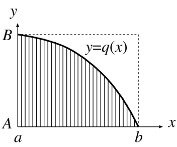
with giving its strict error bound. Here, q⁡(x)q(x) is a monotone function that may have derivative singularity at the endpoints of [a,b][a,\,b], and the integrand f⁡(x,y)f(x,y) also may have singularity on the boundary of the square region [a,b]×[A,B][a,\,b]\times[A,\,B] (see also Figs. 2 and 2). In this case, a Cartesian product rule of a well known one-dimensional quadrature formula (such as the Gaussian formula and the Clenshaw–Curtis formula) does not work properly, or at least its mathematically-rigorous error bound is quite difficult to obtain, because such formulas require the analyticity of the integrand in a neighbourhood of the boundary [1].

Refer to caption
Figure 1: The domain of integration (1.1) when q′​(x)≥0q^{\prime}(x)\geq 0.

Refer to caption
Figure 2: The domain of integration (1.1) when q′​(x)≤0q^{\prime}(x)\leq 0.

Promising quadrature formulas that does not require the analyticity at the endpoints may include the tanh formula [15], the IMT formula [3, 4], and the double-exponential formula [20], which enjoy exponential convergence whether the integrand has such singularity or not. Actually, based on the IMT formula, an automatic integration algorithm for (1.1) was developed [12]. Further improved version was developed as d2lri [2] and r2d2lri [13], where the lattice rule is employed with the IMT transformation [3, 4] or the Sidi transformation [16, 17]. As a related study, based on the double-exponential formula, an automatic integration algorithm over a sphere was developed [14], which also intended to deal with such integrand singularity. The efficiency of those algorithms are also suggested by their numerical experiments.

From a mathematical viewpoint, however, those algorithms do not guarantee the accuracy of the approximation in reality. In order to estimate the error (for giving a stop criterion), Robinson and de Doncker [12] considered the sequence of the number of function evaluation points {Nm}m\{N_{m}\}_{m} and that of approximation values {INm}\{I_{N_{m}}\}, and made the important assumption:

DNm:=|INm−INm−1|≃|I−INm−1|,D_{N_{m}}:=|I_{N_{m}}-I_{N_{m-1}}|\simeq|I-I_{N_{m-1}}|, (1.2)

which enables the error estimation |I−INm|≃DNm2/DNm−1|I-I_{N_{m}}|\simeq D_{N_{m}}^{2}/D_{N_{m-1}}. Similar approach was taken in the studies described above [2, 13, 14]. The problem here is that it is quite difficult to guarantee the validity of (1.2), although it had been widely accepted as a realistic practical assumption for constructing automatic quadrature routines in that period. The recent trend is that the approximation error is bounded by a strict inequality (instead of estimation ‘≃\simeq’) as

|I−IN|≤EN,|I-I_{N}|\leq E_{N},

where ENE_{N} is given in a computable form (see, for example, Petras [11]). Such an explicit error bound is desired for constructing a more reliable, verified numerical integration routine. In addition to the mathematical rigorousness, such a bound gives us another advantage: the sufficient number of NN for the required precision, say N0N_{0}, can be known without generating the sequence {IN}\{I_{N}\}. This means low computational cost, since we do not have to compute for any NN with N<N0N<N_{0} (and of course N>N0N>N_{0}).

The objective of this study is to give such an explicit error bound for the numerical integration method developed by Muhammad–Mori [7]. Their method is based on the Sinc methods [18, 19] combined with double-exponential transformation [5, 20], and it has the following two features:

  1. 1.

    it has beautiful exponential accuracy even if f⁡(x,y)f(x,y) or q⁡(x)q(x) has boundary singularity, and

  2. 2.

    it employs indefinite integration formula instead of quadrature formula for the inner integral.

The first point is the same feature as the studies above [12, 14], but the second point is a unique one. If a standard quadrature rule is employed to approximate the inner integral, the weight wjw_{j} and quadrature node yjy_{j} should be adjusted depending on xx as

∫Aq⁡(x)f⁡(x,y)​𝑑y≈∑jwj​(x)​f​(x,yj​(x)),\int_{A}^{q(x)}f(x,y)\,\mathrm{d}y\approx\sum_{j}w_{j}(x)f(x,y_{j}(x)),

whereas in the case of an indefinite integration formula, yjy_{j} is fixed (independent of xx) as

∫Aq⁡(x)f⁡(x,y)​𝑑y≈∑jwj​(x)​f​(x,yj).\int_{A}^{q(x)}f(x,y)\,\mathrm{d}y\approx\sum_{j}w_{j}(x)f(x,y_{j}).

This independency on xx is quite useful to check mathematical assumptions on the integrand f⁡(x,y)f(x,y) for the exponential accuracy. Furthermore, as a special case, when the integrand is of a product type: f⁡(x,y)=X⁡(x)​Y​(y)f(x,y)=X(x)Y(y), the number of function evaluation to approximate (1.1) is drastically dropped from O⁡(n×n)\Order(n\times n) to O⁡(n+n)\Order(n+n), where nn denotes the number of the terms of ∑\sum (it is also emphasized in the original paper [7]).

However, rigorous error analysis is not given for the formula, and there is room for improvement in the convergence rate. Moreover, it cannot handle the case q′​(x)≤0q^{\prime}(x)\leq 0 (only the case q′​(x)≥0q^{\prime}(x)\geq 0 is considered). In order to reinforce their formula, this study contributes in the following points:

  1. 3.

    their formula is modified so that it can achieve a better convergence rate in both cases (i.e., the case q′​(x)≥0q^{\prime}(x)\geq 0 and q′​(x)≤0q^{\prime}(x)\leq 0), and

  2. 4.

    a rigorous, explicit error bound is given for the modified formula.

From the error bound in the latter point, we can see that the convergence rate of the formula is generally O(exp(−cn/log(γn)))\Order(\exp(-c\sqrt{n}/\log(\gamma\sqrt{n}))), and if f⁡(x,y)=X⁡(x)​Y​(y)f(x,y)=X(x)Y(y), it becomes O(exp(−c′n/log(γ′n)))\Order(\exp(-c^{\prime}n/\log(\gamma^{\prime}n))).

The remainder of this paper is organized as follows. In Section 2, after the review of basic formulas of Sinc methods, Muhammad-Mori’s original formula [7] is described. Then, the formula is modified in Section 3, and its explicit error bound is also presented. Its proof is given in Section 5. Numerical examples are shown in Section 4. Section 6 is devoted to conclusion.

2 Review of Muhammad–Mori’s approximation formula

In this section, the approximation formula for (1.1) derived by Muhammad–Mori [7] is described. The idea is to use “Sinc quadrature” for the outer integral, and to use “Sinc indefinite integration” for the inner integral. Those two approximation formulas are explained first.

2.1 Sinc quadrature and Sinc indefinite integration combined with the DE transformation

The Sinc quadrature and Sinc indefinite integration are approximation formulas for definite integration and indefinite integration, respectively, expressed as

∫−∞∞G⁡(ξ)​𝑑ξ\displaystyle\int_{-\infty}^{\infty}G(\xi)\,\mathrm{d}\xi ≈h~​∑i=−M−M+G⁡(i​h~),\displaystyle\approx\tilde{h}\sum_{i=-M_{-}}^{M_{+}}G(i\tilde{h}), (2.1)
∫−∞ξG⁡(η)​𝑑η\displaystyle\int_{-\infty}^{\xi}G(\eta)\,\mathrm{d}\eta ≈∑j=−N−N+G⁡(j​h)​J​(j,h)​(ξ),ξ∈ℝ,\displaystyle\approx\sum_{j=-N_{-}}^{N_{+}}G(jh)J(j,h)(\xi),\quad\xi\in\mathbb{R}, (2.2)

where J​(j,h)​(ξ)J(j,h)(\xi) is defined by using the so-called sine integral Si⁡(x)=∫0x{(sin⁡σ)/σ}​𝑑σ\Si(x)=\int_{0}^{x}\{(\sin\sigma)/\sigma\}\,\mathrm{d}\sigma as

J⁡(j,h)​(ξ)=h⁡{12+1π​Si⁡[π⁡(ξ/h−j)]}.J(j,h)(\xi)=h\left\{\frac{1}{2}+\frac{1}{\piup}\Si[\piup(\xi/h-j)]\right\}.

Although the formulas (2.1) and (2.2) are approximations on the whole real line ℝ\mathbb{R}, those can be used on the finite interval (a,b)(a,\,b) as well, by using the Double-Exponential (DE) transformation

x=ψDE​(ξ)\displaystyle x=\psi_{\text{\tiny{\rm{DE}}}}(\xi) =b−a2​tanh⁡(π2​sinh⁡ξ)+b+a2.\displaystyle=\frac{b-a}{2}\tanh\left(\frac{\piup}{2}\sinh\xi\right)+\frac{b+a}{2}.

Since ψDE:ℝ→(a,b)\psi_{\text{\tiny{\rm{DE}}}}:\mathbb{R}\to(a,\,b), we can apply the formulas (2.1) and (2.2) in the case of finite intervals combining the DE transformation as

∫abg⁡(x)​𝑑x\displaystyle\int_{a}^{b}g(x)\,\mathrm{d}x =∫−∞∞g⁡(ψDE​(ξ))​ψDE′​(ξ)​𝑑ξ≈h~​∑i=−M−M+g⁡(ψDE​(i​h~))​ψDE′​(i​h~),\displaystyle=\int_{-\infty}^{\infty}g(\psi_{\text{\tiny{\rm{DE}}}}(\xi))\psi_{\text{\tiny{\rm{DE}}}}^{\prime}(\xi)\,\mathrm{d}\xi\approx\tilde{h}\sum_{i=-M_{-}}^{M_{+}}g(\psi_{\text{\tiny{\rm{DE}}}}(i\tilde{h}))\psi_{\text{\tiny{\rm{DE}}}}^{\prime}(i\tilde{h}), (2.3)
∫axg⁡(y)​𝑑y\displaystyle\int_{a}^{x}g(y)\,\mathrm{d}y =∫−∞ψDE−1​(x)g⁡(ψDE​(η))​ψDE′​(η)​𝑑η≈∑j=−N−N+g⁡(ψDE​(j​h))​ψDE′​(j​h)​J​(j,h)​(ψDE−1​(x)),x∈(a,b),\displaystyle=\int_{-\infty}^{\psi_{\text{\tiny{\rm{DE}}}}^{-1}(x)}g(\psi_{\text{\tiny{\rm{DE}}}}(\eta))\psi_{\text{\tiny{\rm{DE}}}}^{\prime}(\eta)\,\mathrm{d}\eta\approx\sum_{j=-N_{-}}^{N_{+}}g(\psi_{\text{\tiny{\rm{DE}}}}(jh))\psi_{\text{\tiny{\rm{DE}}}}^{\prime}(jh)J(j,h)(\psi_{\text{\tiny{\rm{DE}}}}^{-1}(x)),\quad x\in(a,\,b), (2.4)

which are called the “DE-Sinc quadrature” and the “DE-Sinc indefinite integration,” proposed by Takahasi–Mori [20] and Muhammad–Mori [6], respectively.

2.2 Muhammad–Mori’s approximation formula

Let the domain of integration (1.1) be as in Fig. 2, i.e., q⁡(a)=Aq(a)=A, q⁡(b)=Bq(b)=B, and q′​(x)≥0q^{\prime}(x)\geq 0. Using the monotonicity of q⁡(x)q(x), Muhammad–Mori [7] rewrote the given integral II by applying y=q⁡(s)y=q(s) as

I=∫ab(∫Aq⁡(x)f⁡(x,y)​𝑑y)​𝑑x=∫ab(∫axf⁡(x,q⁡(s))​q′​(s)​𝑑s)​𝑑x.I=\int_{a}^{b}\left(\int_{A}^{q(x)}f(x,y)\,\mathrm{d}y\right)\,\mathrm{d}x=\int_{a}^{b}\left(\int_{a}^{x}f(x,q(s))q^{\prime}(s)\,\mathrm{d}s\right)\,\mathrm{d}x. (2.5)

Note that s∈(a,b)s\in(a,\,b) (i.e., not (A,B)(A,\,B)). Then, they applied (2.3) and (2.4), with taking h~=h\tilde{h}=h, M−=M+=mM_{-}=M_{+}=m, and N−=N+=nN_{-}=N_{+}=n for simplicity, as follows:

I\displaystyle I ≈h​∑i=−mmψDE′​(i​h)​(∫aψDE​(i​h)f⁡(ψDE​(i​h),q⁡(s))​q′​(s)​𝑑s)\displaystyle\approx h\sum_{i=-m}^{m}\psi_{\text{\tiny{\rm{DE}}}}^{\prime}(ih)\left(\int_{a}^{\psi_{\text{\tiny{\rm{DE}}}}(ih)}f(\psi_{\text{\tiny{\rm{DE}}}}(ih),q(s))q^{\prime}(s)\,\mathrm{d}s\right)
≈h​∑i=−mmψDE′​(i​h)​{∑j=−nnf⁡(ψDE​(i​h),q⁡(ψDE​(j​h)))​q′​(ψDE​(j​h))​ψDE′​(j​h)​J​(j,h)​(i​h)}.\displaystyle\approx h\sum_{i=-m}^{m}\psi_{\text{\tiny{\rm{DE}}}}^{\prime}(ih)\left\{\sum_{j=-n}^{n}f(\psi_{\text{\tiny{\rm{DE}}}}(ih),q(\psi_{\text{\tiny{\rm{DE}}}}(jh)))q^{\prime}(\psi_{\text{\tiny{\rm{DE}}}}(jh))\psi_{\text{\tiny{\rm{DE}}}}^{\prime}(jh)J(j,h)(ih)\right\}.

If we introduce xi=ψDE​(i​h)x_{i}=\psi_{\text{\tiny{\rm{DE}}}}(ih), wj=π​cosh⁡(j​h)​sech2⁡(π​sinh⁡(j​h)/2)/4w_{j}=\piup\cosh(jh)\sech^{2}(\piup\sinh(jh)/2)/4, and σk=Si⁡[π​k]/π\sigma_{k}=\Si[\piup k]/\piup, which can be prepared in prior to computation (see also a value table for σk\sigma_{k} [18, Table 1.10.1]), the formula is rewritten as

I≈(b−a)2​h2​∑i=−mmwi​{∑j=−nnf⁡(xi,q⁡(xj))​q′​(xj)​wj​(12+σi−j)}.I\approx(b-a)^{2}h^{2}\sum_{i=-m}^{m}w_{i}\left\{\sum_{j=-n}^{n}f(x_{i},q(x_{j}))q^{\prime}(x_{j})w_{j}\left(\frac{1}{2}+\sigma_{i-j}\right)\right\}. (2.6)

The total number of function evaluations, say NtotalN_{\text{total}}, of this formula is Ntotal=(2​m+1)×(2​n+1)N_{\text{total}}=(2m+1)\times(2n+1). As a special case, if the integrand is of a product type: f⁡(x,y)=X⁡(x)​Y​(y)f(x,y)=X(x)Y(y), the formula is rewritten as

I≈(b−a)2​h2​∑i=−mmU⁡(i)​{∑j=−nnV⁡(j)​(12+σi−j)},\displaystyle I\approx(b-a)^{2}h^{2}\sum_{i=-m}^{m}U(i)\left\{\sum_{j=-n}^{n}V(j)\left(\frac{1}{2}+\sigma_{i-j}\right)\right\}, (2.7)

where U⁡(i)=X⁡(xi)​wiU(i)=X(x_{i})w_{i} and V⁡(j)=Y⁡(q⁡(xj))​q′​(xj)​wjV(j)=Y(q(x_{j}))q^{\prime}(x_{j})w_{j}. In this case, we can see that Ntotal=(2​m+1)+(2​n+1)N_{\text{total}}=(2m+1)+(2n+1), which is significantly smaller than (2​m+1)×(2​n+1)(2m+1)\times(2n+1).

They [7] also roughly discussed the error rate of the formula (2.6) as follows. Let 𝒟d\mathscr{D}_{d} be a strip domain defined by 𝒟d={ζ∈ℂ:|Imζ|<d}\mathscr{D}_{d}=\{\zeta\in\mathbb{C}:|\mathop{\mathrm{Im}}\nolimits\zeta|<d\} for d>0d>0. Assume that the integrand gg in (2.3) and (2.4) is analytic on ψDE​(𝒟d)\psi_{\text{\tiny{\rm{DE}}}}(\mathscr{D}_{d}) (which means g​(ψDE​(⋅))g(\psi_{\text{\tiny{\rm{DE}}}}(\cdot)) is analytic on 𝒟d\mathscr{D}_{d}), and further assume that g⁡(x)g(x) behaves O⁡(((x−a)​(b−x))ν−1)\Order(((x-a)(b-x))^{\nu-1}) (ν>0\nu>0) as x→ax\to a and x→bx\to b. Under the assumptions with some additional mild conditions, it is known that the approximation (2.3) converges with O(e−2πd/h)\Order(\rme^{-2\piup d/h}), and the approximation (2.4) converges with O(he−πd/h)\Order(h\rme^{-\piup d/h}), by taking h=h~h=\tilde{h} and

M+=M−=m=⌈1h​log⁡(4​d(ν−ϵ)​h)⌉,N+=N−=n=⌈1h​log⁡(2​d(ν−ϵ)​h)⌉,M_{+}=M_{-}=m=\left\lceil\frac{1}{h}\log\left(\frac{4d}{(\nu-\epsilon)h}\right)\right\rceil,\quad N_{+}=N_{-}=n=\left\lceil\frac{1}{h}\log\left(\frac{2d}{(\nu-\epsilon)h}\right)\right\rceil,

where ϵ\epsilon is an arbitrary small positive number. Therefore, if the same assumptions are satisfied for both approximations in (2.6), it enjoys exponential accuracy: O(he−πd/h)\Order(h\rme^{-\piup d/h}). Since m≃n≃Ntotal/4m\simeq n\simeq\sqrt{N_{\text{total}}/4} and h≃log⁡(c​n)/nh\simeq\log(cn)/n (where c=2​d/(ν−ϵ)c=2d/(\nu-\epsilon)), this can be interpreted in terms of NtotalN_{\text{total}} as

O⁡(log⁡(c​Ntotal/4)Ntotal/4​exp⁡[−π​d​Ntotal/4log⁡(c​Ntotal/4)]).\Order\left(\frac{\log(c\sqrt{N_{\text{total}}/4})}{\sqrt{N_{\text{total}}/4}}\exp\left[\frac{-\piup d\sqrt{N_{\text{total}}/4}}{\log(c\sqrt{N_{\text{total}}/4})}\right]\right). (2.8)

If the integrand is of a product type, since m≃n≃Ntotal/4m\simeq n\simeq N_{\text{total}}/4, it becomes

O⁡(log⁡(c​Ntotal/4)Ntotal/4​exp⁡[−π​d​(Ntotal/4)log⁡(c​Ntotal/4)]).\Order\left(\frac{\log(cN_{\text{total}}/4)}{N_{\text{total}}/4}\exp\left[\frac{-\piup d(N_{\text{total}}/4)}{\log(cN_{\text{total}}/4)}\right]\right). (2.9)

Although the convergence rate was roughly discussed as above, the quantity of the approximation error cannot be obtained because rigorous error bound was not given. Moreover, the case q′​(x)≤0q^{\prime}(x)\leq 0 (cf. Fig. 2) is not considered. This situation will be improved in the next section.

3 Main results: modified approximation formula and its explicit error bound

This section is devoted to a description of a new approximation formula and its error bound. The proof of the error bound is given in Section 5.

3.1 Modified approximation formula

In the approximations (2.3) and (2.4), Muhammad–Mori [7] set the mesh size as h~=h\tilde{h}=h for simplicity, but here, h~\tilde{h} is selected as h~=2​h\tilde{h}=2h. Furthermore, both M−=M+M_{-}=M_{+} and N−=N+N_{-}=N_{+} are not assumed. Then, after applying y=q⁡(s)y=q(s) as in (2.5), the modified formula is derived as

I\displaystyle I ≈2​h​∑i=−M−M+ψDE′​(2​i​h)​(∫aψDE​(2​i​h)f⁡(ψDE​(2​i​h),q⁡(s))​q′​(s)​𝑑s)\displaystyle\approx 2h\sum_{i=-M_{-}}^{M_{+}}\psi_{\text{\tiny{\rm{DE}}}}^{\prime}(2ih)\left(\int_{a}^{\psi_{\text{\tiny{\rm{DE}}}}(2ih)}f(\psi_{\text{\tiny{\rm{DE}}}}(2ih),q(s))q^{\prime}(s)\,\mathrm{d}s\right)
≈2​h​∑i=−M−M+ψDE′​(2​i​h)​{∑j=−N−N+f⁡(ψDE​(2​i​h),q⁡(ψDE​(j​h)))​q′​(ψDE​(j​h))​ψDE′​(j​h)​J​(j,h)​(2​i​h)},\displaystyle\approx 2h\sum_{i=-M_{-}}^{M_{+}}\psi_{\text{\tiny{\rm{DE}}}}^{\prime}(2ih)\left\{\sum_{j=-N_{-}}^{N_{+}}f(\psi_{\text{\tiny{\rm{DE}}}}(2ih),q(\psi_{\text{\tiny{\rm{DE}}}}(jh)))q^{\prime}(\psi_{\text{\tiny{\rm{DE}}}}(jh))\psi_{\text{\tiny{\rm{DE}}}}^{\prime}(jh)J(j,h)(2ih)\right\},

which can be rewritten as

I≈IDEinc​(h):=2​(b−a)2​h2​∑i=−M−M+w2​i​{∑i=−N−N+f⁡(x2​i,q⁡(xj))​q′​(xj)​wj​(12+σ2​i−j)}.I\approx I_{\text{\tiny{\rm{DE}}}}^{\text{\rm{inc}}}(h):=2(b-a)^{2}h^{2}\sum_{i=-M_{-}}^{M_{+}}w_{2i}\left\{\sum_{i=-N_{-}}^{N_{+}}f(x_{2i},q(x_{j}))q^{\prime}(x_{j})w_{j}\left(\frac{1}{2}+\sigma_{2i-j}\right)\right\}. (3.1)

The positive integers M±M_{\pm} and N±N_{\pm} are also selected depending on hh, which is explained in the subsequent theorem that states the error bound.

The formula (3.1) is derived in the case q′​(x)≥0q^{\prime}(x)\geq 0 (cf. Fig. 2), but in the case q′​(x)≤0q^{\prime}(x)\leq 0 (cf. Fig. 2) as well, we can derive the similar formula as follows. First, applying y=q⁡(s)y=q(s), we have

I=∫ab(∫Aq⁡(x)f⁡(x,y)​𝑑y)​𝑑x\displaystyle I=\int_{a}^{b}\left(\int_{A}^{q(x)}f(x,y)\,\mathrm{d}y\right)\,\mathrm{d}x =∫ab(∫xbf⁡(x,q⁡(s))​{−q′​(s)}​𝑑s)​𝑑x\displaystyle=\int_{a}^{b}\left(\int_{x}^{b}f(x,q(s))\{-q^{\prime}(s)\}\,\mathrm{d}s\right)\,\mathrm{d}x
=∫ab(∫abf⁡(x,q⁡(s))​{−q′​(s)}​𝑑s−∫axf⁡(x,q⁡(s))​{−q′​(s)}​𝑑s)​𝑑x.\displaystyle=\int_{a}^{b}\left(\int_{a}^{b}f(x,q(s))\{-q^{\prime}(s)\}\,\mathrm{d}s-\int_{a}^{x}f(x,q(s))\{-q^{\prime}(s)\}\,\mathrm{d}s\right)\,\mathrm{d}x.

Then, apply (2.3) and (2.4) to obtain

I≈2​h​∑i=−M−M+ψDE′​(2​i​h)​{∑j=−N−N+f⁡(ψDE​(2​i​h),q⁡(ψDE​(j​h)))​{−q′​(ψDE​(j​h))}​ψDE′​(j​h)​(h−J⁡(j,h)​(2​i​h))}.I\approx 2h\sum_{i=-M_{-}}^{M_{+}}\psi_{\text{\tiny{\rm{DE}}}}^{\prime}(2ih)\left\{\sum_{j=-N_{-}}^{N_{+}}f(\psi_{\text{\tiny{\rm{DE}}}}(2ih),q(\psi_{\text{\tiny{\rm{DE}}}}(jh)))\{-q^{\prime}(\psi_{\text{\tiny{\rm{DE}}}}(jh))\}\psi_{\text{\tiny{\rm{DE}}}}^{\prime}(jh)\left(h-J(j,h)(2ih)\right)\right\}.

Here, limξ→∞J⁡(j,h)​(ξ)=h\lim_{\xi\to\infty}J(j,h)(\xi)=h is used. This approximation can be rewritten as

I≈IDEdec​(h):=2​(b−a)2​h2​∑i=−M−M+w2​i​{∑i=−N−N+f⁡(x2​i,q⁡(xj))​{−q′​(xj)}​wj​(12−σ2​i−j)}.I\approx I_{\text{\tiny{\rm{DE}}}}^{\text{\rm{dec}}}(h):=2(b-a)^{2}h^{2}\sum_{i=-M_{-}}^{M_{+}}w_{2i}\left\{\sum_{i=-N_{-}}^{N_{+}}f(x_{2i},q(x_{j}))\{-q^{\prime}(x_{j})\}w_{j}\left(\frac{1}{2}-\sigma_{2i-j}\right)\right\}. (3.2)

The formulas (3.1) and (3.2) inherit the advantage of Muhammad–Mori’s one in the sense that Ntotal=(M−+M++1)×(N−+N++1)N_{\text{total}}=(M_{-}+M_{+}+1)\times(N_{-}+N_{+}+1) in general, but if the integrand is of a product type: f⁡(x,y)=X⁡(x)​Y​(y)f(x,y)=X(x)Y(y), it becomes Ntotal=(M−+M++1)+(N−+N++1)N_{\text{total}}=(M_{-}+M_{+}+1)+(N_{-}+N_{+}+1), which is easily confirmed by rewriting it in the same way as (2.7). Furthermore, it also inherits (or even enhances) the exponential accuracy, which is described next.

3.2 Explicit error bound of the modified formula

For positive constants κ\kappa, λ\lambda and dd with 0<d<π/20<d<\piup/2, let us define cκ,λ,dc_{\kappa,\lambda,d} as

cκ,λ,d=1cosκ+λ⁡(π2​sin⁡d)​cos⁡d,c_{\kappa,\lambda,d}=\frac{1}{\cos^{\kappa+\lambda}(\frac{\piup}{2}\sin d)\cos d},

and define ρκ\rho_{\kappa} as

ρκ={arcsinh⁡(1+1−(2​π​κ)22​π​κ)(0<κ<1/(2​π)),arcsinh⁡(1)(1/(2​π)≤κ).\rho_{\kappa}=\begin{cases}\arcsinh\left(\frac{\sqrt{1+\sqrt{1-(2\piup\kappa)^{2}}}}{2\piup\kappa}\right)&(0<\kappa<1/(2\piup)),\\ \arcsinh(1)&(1/(2\piup)\leq\kappa).\end{cases}

Then, the errors of IDEinc​(h)I_{\text{\tiny{\rm{DE}}}}^{\text{\rm{inc}}}(h) and IDEdec​(h)I_{\text{\tiny{\rm{DE}}}}^{\text{\rm{dec}}}(h) are estimated as stated below.

Theorem 3.1

Let α\alpha, β\beta, γ\gamma, δ\delta, and KK be positive constants, and dd be a constant with 0<d<π/20<d<\piup/2. Assume the following conditions:

  1. 1.

    qq is analytic and bounded in ψDE​(𝒟d)\psi_{\text{\tiny{\rm{DE}}}}(\mathscr{D}_{d}),

  2. 2.

    f⁡(⋅,q⁡(w))f(\cdot,q(w)) is analytic in ψDE​(𝒟d)\psi_{\text{\tiny{\rm{DE}}}}(\mathscr{D}_{d}) for all w∈ψDE​(𝒟d)w\in\psi_{\text{\tiny{\rm{DE}}}}(\mathscr{D}_{d}),

  3. 3.

    f⁡(z,q⁡(⋅))f(z,q(\cdot)) is analytic in ψDE​(𝒟d)\psi_{\text{\tiny{\rm{DE}}}}(\mathscr{D}_{d}) for all z∈ψDE​(𝒟d)z\in\psi_{\text{\tiny{\rm{DE}}}}(\mathscr{D}_{d}),

  4. 4.

    it holds for all z∈ψDE​(𝒟d)z\in\psi_{\text{\tiny{\rm{DE}}}}(\mathscr{D}_{d}) and w∈ψDE​(𝒟d)w\in\psi_{\text{\tiny{\rm{DE}}}}(\mathscr{D}_{d}) that

    |f⁡(z,q⁡(w))​q′​(w)|≤K​|z−a|α−1​|b−z|β−1​|w−a|γ−1​|b−w|δ−1.|f(z,q(w))q^{\prime}(w)|\leq K|z-a|^{\alpha-1}|b-z|^{\beta-1}|w-a|^{\gamma-1}|b-w|^{\delta-1}. (3.3)

Let μ=min⁡{α,β}{\mu}=\min\{\alpha,\beta\}, μ¯=max⁡{α,β}\overline{\mu}=\max\{\alpha,\beta\}, ν=min⁡{γ,δ}{\nu}=\min\{\gamma,\delta\}, ν¯=max⁡{γ,δ}\overline{\nu}=\max\{\gamma,\delta\}, let h~=2​h\tilde{h}=2h, let nn and mm be positive integers defined by

n=⌈1h​log⁡(2​dν​h)⌉,m=⌈12​{n+1h​log⁡(μν)}⌉,n=\left\lceil\frac{1}{h}\log\left(\frac{2d}{\nu h}\right)\right\rceil,\quad m=\left\lceil\frac{1}{2}\left\{n+\frac{1}{h}\log\left(\frac{\mu}{\nu}\right)\right\}\right\rceil, (3.4)

and let M−M_{-} and M+M_{+} be positive integers defined by

{M−=m,M+=m−⌊log⁡(β/α)/h~⌋(if​μ=α),M+=m,M−=m−⌊log⁡(α/β)/h~⌋(if​μ=β),\begin{cases}M_{-}=m,\quad M_{+}=m-\lfloor\log(\beta/\alpha)/\tilde{h}\rfloor&\quad(\text{if}\,\,\,\mu=\alpha),\\ M_{+}=m,\quad M_{-}=m-\lfloor\log(\alpha/\beta)/\tilde{h}\rfloor&\quad(\text{if}\,\,\,\mu=\beta),\end{cases} (3.5)

and let N−N_{-} and N+N_{+} be positive integers defined by

{N−=n,N+=n−⌊log⁡(δ/γ)/(h)⌋(if​ν=γ),N+=n,N−=n−⌊log⁡(γ/δ)/(h)⌋(if​ν=δ),\begin{cases}N_{-}=n,\quad N_{+}=n-\lfloor\log(\delta/\gamma)/(h)\rfloor&\quad(\text{if}\,\,\,\nu=\gamma),\\ N_{+}=n,\quad N_{-}=n-\lfloor\log(\gamma/\delta)/(h)\rfloor&\quad(\text{if}\,\,\,\nu=\delta),\end{cases} (3.6)

and let hh (>0)(>0) be taken sufficiently small so that

M−​h~≥ρα,M+​h~≥ρβ,N−​h≥ργ,N+​h≥ρδM_{-}\tilde{h}\geq\rho_{\alpha},\quad M_{+}\tilde{h}\geq\rho_{\beta},\quad N_{-}h\geq\rho_{\gamma},\quad N_{+}h\geq\rho_{\delta}

are all satisfied. Then, if q′​(x)≥0q^{\prime}(x)\geq 0, it holds that

|I−IDEinc​(h)|\displaystyle|I-I_{\text{\tiny{\rm{DE}}}}^{\text{\rm{inc}}}(h)|
≤[B⁡(γ,δ)​cγ,δ,dμ​{eπ2​μ¯+2​cα,β,d1−e−πd/h}+1ν​{B⁡(α,β)+4​cα,β,dμ​e−πd/h1−e−πd/h}​{1.1​eπ2​ν¯+h​cγ,δ,dd(1−e−2πd/h)}]\displaystyle\leq\left[\frac{\Bfunc(\gamma,\delta)c_{\gamma,\delta,d}}{\mu}\left\{\rme^{\frac{\piup}{2}\overline{\mu}}+\frac{2c_{\alpha,\beta,d}}{1-\rme^{-\piup d/h}}\right\}+\frac{1}{\nu}\left\{\Bfunc(\alpha,\beta)+\frac{4c_{\alpha,\beta,d}}{\mu}\frac{\rme^{-\piup d/h}}{1-\rme^{-\piup d/h}}\right\}\left\{1.1\rme^{\frac{\piup}{2}\overline{\nu}}+\frac{hc_{\gamma,\delta,d}}{d(1-\rme^{-2\piup d/h})}\right\}\right]
×2K(b−a)α+β+γ+δ−2e−πd/h,\displaystyle\quad\times 2K(b-a)^{\alpha+\beta+\gamma+\delta-2}\rme^{-\piup d/h}, (3.7)

where B⁡(κ,λ)\Bfunc(\kappa,\lambda) is the beta function. If q′​(x)≤0q^{\prime}(x)\leq 0, |I−IDEdec​(h)||I-I_{\text{\tiny{\rm{DE}}}}^{\text{\rm{dec}}}(h)| is bounded by the same term on the right hand side of (3.7).

The convergence rate of (3.7) is O(e−πd/h)\Order(\rme^{-\piup d/h}), which can be interpreted in terms of NtotalN_{\text{total}} as follows. Since n≃N−≃N+n\simeq N_{-}\simeq N_{+} and m≃M−≃M+≃(n/2)m\simeq M_{-}\simeq M_{+}\simeq(n/2), we can see Ntotal≃((n/2)+(n/2)+1)​(n+n+1)≃2​n2N_{\text{total}}\simeq((n/2)+(n/2)+1)(n+n+1)\simeq 2n^{2}. From this and h≃log⁡(c′​n)/nh\simeq\log(c^{\prime}n)/n (where c′=2​d/νc^{\prime}=2d/\nu), the convergence rate of the modified formula is

O⁡(exp⁡[−π​d​Ntotal/2log⁡(c′​Ntotal/2)]).\Order\left(\exp\left[\frac{-\piup d\sqrt{N_{\text{total}}/2}}{\log(c^{\prime}\sqrt{N_{\text{total}}/2})}\right]\right).

This rate is better than Muhammad–Mori’s one (2.8). If the integrand is of a product type: f⁡(x,y)=X⁡(x)​Y​(y)f(x,y)=X(x)Y(y), it becomes

O⁡(exp⁡[−π​d​(Ntotal/3)log⁡(c​Ntotal/3)]),\Order\left(\exp\left[\frac{-\piup d(N_{\text{total}}/3)}{\log(cN_{\text{total}}/3)}\right]\right),

since Ntotal≃((n/2)+(n/2)+1)+(n+n+1)≃3​nN_{\text{total}}\simeq((n/2)+(n/2)+1)+(n+n+1)\simeq 3n in this case. This rate is also better than Muhammad–Mori’s one (2.9).

Remark 1

The inequality (3.7) states the bound of the absolute error, say Eabs​(h)E^{\text{\rm{abs}}}(h). If necessary, the bound of the relative error Erel​(h)E^{\text{\rm{rel}}}(h) is also obtained as follows:

Erel​(h)=|I−IDEinc​(h)||I|≤|Eabs​(h)||I|≤|Eabs​(h)|||IDEinc​(h)|−Eabs​(h)|.E^{\text{\rm{rel}}}(h)=\frac{|I-I_{\text{\tiny{\rm{DE}}}}^{\text{\rm{inc}}}(h)|}{|I|}\leq\frac{|E^{\text{\rm{abs}}}(h)|}{|I|}\leq\frac{|E^{\text{\rm{abs}}}(h)|}{||I_{\text{\tiny{\rm{DE}}}}^{\text{\rm{inc}}}(h)|-E^{\text{\rm{abs}}}(h)|}.

4 Numerical examples

In this section, numerical results of Muhammad-Mori’s original formula [7] and modified formula are presented. The results of an existing library: r2d2lri [13], which can properly handle boundary singularity in q⁡(x)q(x) and f⁡(x,y)f(x,y), are also shown. The computation was done on Mac OS X 10.6, Mac Pro two 2.93 GHz 6-Core Intel Xeon with 32 GB DDR3 ECC SDRAM. The computation programs were implemented in C/C++ with double-precision floating-point arithmetic, and compiled by GCC 4.0.1 with no optimization. The following three examples were conducted.

Example 1 (The integrand and boundary function are smooth [7, Example 2])
∫02(∫0x2/2d​yx+y+(1/2))​𝑑x=−(2+12)​log⁡(1+2​2)+2​(1+2)​log⁡(1+2)−2.\int_{0}^{\sqrt{2}}\left(\int_{0}^{x^{2}/2}\frac{\mathrm{d}y}{x+y+(1/2)}\right)\,\mathrm{d}x=-\left(\sqrt{2}+\frac{1}{2}\right)\log\left(1+2\sqrt{2}\right)+2\left(1+\sqrt{2}\right)\log\left(1+\sqrt{2}\right)-\sqrt{2}.
Example 2 (Derivative singularity exists in the integrand and boundary function [7, Example 1])
∫01(∫01−(1−x)21−y2​𝑑y)​𝑑x=23.\int_{0}^{1}\left(\int_{0}^{\sqrt{1-(1-x)^{2}}}\sqrt{1-y^{2}}\,\mathrm{d}y\right)\,\mathrm{d}x=\frac{2}{3}.
Example 3 (The integrand is weakly singular at the origin [2, Example 27])
∫01(∫01−xd​yx​y)​𝑑x=π.\int_{0}^{1}\left(\int_{0}^{1-x}\frac{\mathrm{d}y}{\sqrt{xy}}\right)\,\mathrm{d}x=\piup.

In the case of Example 1, the assumptions in Theorem 3.1 are satisfied with α=β=δ=1\alpha=\beta=\delta=1, γ=2\gamma=2, d=log⁡(2)d=\log(2), and K=16.6K=16.6. The results are shown in Figs. 8 and 8. In both figures, error bound (say E~rel​(h)\tilde{E}^{\text{rel}}(h)) given by Theorem 3.1 surely includes the observed relative error Erel​(h)E^{\text{rel}}(h) in the form Erel​(h)≤E~rel​(h)E^{\text{rel}}(h)\leq\tilde{E}^{\text{rel}}(h), which is also true in all the subsequent examples (note that such error bound is not given for Muhammad–Mori’s original formula). In view of the performance, r2d2lri is better than original/modified formulas, but its error estimate just claims Erel​(h)≈E~rel​(h)E^{\text{rel}}(h)\approx\tilde{E}^{\text{rel}}(h), and does not guarantee Erel​(h)≤E~rel​(h)E^{\text{rel}}(h)\leq\tilde{E}^{\text{rel}}(h) mathematically.

In the case of Example 2, the assumptions in Theorem 3.1 are satisfied with α=β=1\alpha=\beta=1, γ=1/2\gamma=1/2, δ=3\delta=3, d=1d=1, and K=1.63K=1.63. The results are shown in Figs. 8 and 8. In this case, the convergence of the original/modified formulas is incredibly fast compared to r2d2lri. This is because the integrand is of a product type: f⁡(x,y)=X⁡(x)​Y​(y)f(x,y)=X(x)Y(y).

The integrand of Example 3 is also of a product type. In this example, the assumptions in Theorem 3.1 are satisfied with α=δ=1/2\alpha=\delta=1/2, β=γ=1\beta=\gamma=1, d=4/3d=4/3, and K=1K=1. The results are shown in Figs. 8 and 8. In this case, the performance of r2d2lri is much worse than that in Example 2, which seems to be due to the singularity of the integrand. In contrast, the modified formula attains the similar convergence rate to that in Example 2. Muhammad–Mori’s original formula cannot be used in this case since q⁡(x)=1−xq(x)=1-x does not satisfy q′​(x)≥0q^{\prime}(x)\geq 0.

Refer to caption
Figure 3: Relative error with respect to NtotalN_{\text{total}} in Example 1.

Refer to caption
Figure 4: Relative error with respect to computation time in Example 1.
Refer to caption
Figure 5: Relative error with respect to NtotalN_{\text{total}} in Example 2.

Refer to caption
Figure 6: Relative error with respect to computation time in Example 2.
Refer to caption
Figure 7: Relative error with respect to NtotalN_{\text{total}} in Example 3.

Refer to caption
Figure 8: Relative error with respect to computation time in Example 3.

5 Proofs

In this section, only the inequality (3.7) (for |I−IDEinc​(h)||I-I_{\text{\tiny{\rm{DE}}}}^{\text{\rm{inc}}}(h)|) is proved, since |I−IDEdec​(h)||I-I_{\text{\tiny{\rm{DE}}}}^{\text{\rm{dec}}}(h)| is bounded in exactly the same way. Let us have a look at the sketch of the proof first.

5.1 Sketch of the proof

The error |I−IDEinc​(h)||I-I_{\text{\tiny{\rm{DE}}}}^{\text{\rm{inc}}}(h)| can be bounded by a sum of two terms as follows:

|I−IDEinc​(h)|\displaystyle|I-I_{\text{\tiny{\rm{DE}}}}^{\text{\rm{inc}}}(h)| ≤|∫abF⁡(x)​𝑑x−h~​∑i=−M−M+F⁡(ψDE​(i​h~))​ψDE′​(i​h~)|\displaystyle\leq\left|\int_{a}^{b}F(x)\,\mathrm{d}x-\tilde{h}\sum_{i=-M_{-}}^{M_{+}}F(\psi_{\text{\tiny{\rm{DE}}}}(i\tilde{h}))\psi_{\text{\tiny{\rm{DE}}}}^{\prime}(i\tilde{h})\right|
+h~∑i=−M−M+ψDE′(ih~)|∫aψDE​(i​h~)fi(s)ds−∑j=−N−N+fi(ψDE(jh))ψDE′(jh)J(j,h)(ih~)|,\displaystyle\quad+\tilde{h}\sum_{i=-M_{-}}^{M_{+}}\psi_{\text{\tiny{\rm{DE}}}}^{\prime}(i\tilde{h})\left|\int_{a}^{\psi_{\text{\tiny{\rm{DE}}}}(i\tilde{h})}f_{i}(s)\,\mathrm{d}s-\sum_{j=-N_{-}}^{N_{+}}f_{i}(\psi_{\text{\tiny{\rm{DE}}}}(jh))\psi_{\text{\tiny{\rm{DE}}}}^{\prime}(jh)J(j,h)(i\tilde{h})\right|,

where F⁡(x)=∫axf⁡(x,q⁡(s))​q′​(s)​𝑑sF(x)=\int_{a}^{x}f(x,q(s))q^{\prime}(s)\,\mathrm{d}s, fi​(s)=f⁡(ψDE​(i​h~),q⁡(s))​q′​(s)f_{i}(s)=f(\psi_{\text{\tiny{\rm{DE}}}}(i\tilde{h}),q(s))q^{\prime}(s), and h~=2​h\tilde{h}=2h. The first term (say E1E_{1}) and the second term (say E2E_{2}) are bounded as follows:

E1\displaystyle E_{1} ≤B⁡(γ,δ)​cγ,δ,dμ{eπ2​μ¯+2​cα,β,d1−e−2πd/h~}2K(b−a)α+β+γ+δ−2e−2πd/h~,\displaystyle\leq\frac{\Bfunc(\gamma,\delta)c_{\gamma,\delta,d}}{\mu}\left\{\rme^{\frac{\piup}{2}\overline{\mu}}+\frac{2c_{\alpha,\beta,d}}{1-\rme^{-2\piup d/\tilde{h}}}\right\}2K(b-a)^{\alpha+\beta+\gamma+\delta-2}\rme^{-2\piup d/\tilde{h}}, (5.1)
E2\displaystyle E_{2} ≤1ν{B(α,β)+4​cα,β,dμe−2πd/h~1−e−2πd/h~}{1.1eπ2​ν¯+h​cγ,δ,dd(1−e−2πd/h)}2K(b−a)α+β+γ+δ−2e−πd/h.\displaystyle\leq\frac{1}{\nu}\left\{\Bfunc(\alpha,\beta)+\frac{4c_{\alpha,\beta,d}}{\mu}\frac{\rme^{-2\piup d/\tilde{h}}}{1-\rme^{-2\piup d/\tilde{h}}}\right\}\left\{1.1\rme^{\frac{\piup}{2}\overline{\nu}}+\frac{hc_{\gamma,\delta,d}}{d(1-\rme^{-2\piup d/h})}\right\}2K(b-a)^{\alpha+\beta+\gamma+\delta-2}\rme^{-\piup d/h}. (5.2)

Then, taking h~=2​h\tilde{h}=2h, we get the desired inequality (3.7). In what follows, the inequalities (5.1) and (5.2) are shown in Sections 5.2 and 5.3, respectively.

5.2 Bound of E1E_{1} (error of the DE-Sinc quadrature)

The following two lemmas are important results for this project.

Lemma 5.2 (Okayama et al. [10, Lemma 4.16])

Let L~\tilde{L}, α\alpha, and β\beta be positive constants, and let μ=min⁡{α,β}\mu=\min\{\alpha,\,\beta\}. Let FF be analytic on ψDE​(𝒟d)\psi_{\text{\tiny{\rm{DE}}}}(\mathscr{D}_{d}) for dd with 0<d<π/20<d<\piup/2, and satisfy

|F⁡(z)|≤L~​|z−a|α−1​|b−z|β−1|F(z)|\leq\tilde{L}|z-a|^{\alpha-1}|b-z|^{\beta-1}

for all z∈ψDE​(𝒟d)z\in\psi_{\text{\tiny{\rm{DE}}}}(\mathscr{D}_{d}). Then it holds that

|∫abF⁡(x)​𝑑x−h~​∑i=−∞∞F⁡(ψDE​(i​h~))​ψDE′​(i​h~)|≤C~1​C~2​e−2πd/h~1−e−2πd/h~,\left|\int_{a}^{b}F(x)\,\mathrm{d}x-\tilde{h}\sum_{i=-\infty}^{\infty}F(\psi_{\text{\tiny{\rm{DE}}}}(i\tilde{h}))\psi_{\text{\tiny{\rm{DE}}}}^{\prime}(i\tilde{h})\right|\leq\tilde{C}_{1}\tilde{C}_{2}\frac{\rme^{-2\piup d/\tilde{h}}}{1-\rme^{-2\piup d/\tilde{h}}},

where the constants C~1\tilde{C}_{1} and C~2\tilde{C}_{2} are defined by

C~1=2​L~​(b−a)α+β−1μ,C~2=2​cα,β,d.\displaystyle\tilde{C}_{1}=\frac{2\tilde{L}(b-a)^{\alpha+\beta-1}}{\mu},\quad\tilde{C}_{2}=2c_{\alpha,\beta,d}. (5.3)
Lemma 5.3 (Okayama et al. [10, Lemma 4.18])

Let the assumptions in Lemma 5.2 be fulfilled. Furthermore, let μ¯=max⁡{α,β}\overline{\mu}=\max\{\alpha,\,\beta\}, let mm be a positive integer, let M−M_{-} and M+M_{+} be positive integers defined by (3.5), and let mm be taken sufficiently large so that M−​h~≥ραM_{-}\tilde{h}\geq\rho_{\alpha} and M+​h~≥ρβM_{+}\tilde{h}\geq\rho_{\beta} hold. Then it holds that

|h~​∑i=−∞−(M−+1)F⁡(ψDE​(i​h~))​ψDE′​(i​h~)+h~​∑i=M++1∞F⁡(ψDE​(i​h~))​ψDE′​(i​h~)|≤eπ2​μ¯⁡C~1​e−π2​μ​exp⁡(m​h~),\left|\tilde{h}\sum_{i=-\infty}^{-(M_{-}+1)}F(\psi_{\text{\tiny{\rm{DE}}}}(i\tilde{h}))\psi_{\text{\tiny{\rm{DE}}}}^{\prime}(i\tilde{h})+\tilde{h}\sum_{i=M_{+}+1}^{\infty}F(\psi_{\text{\tiny{\rm{DE}}}}(i\tilde{h}))\psi_{\text{\tiny{\rm{DE}}}}^{\prime}(i\tilde{h})\right|\leq\rme^{\frac{\piup}{2}\overline{\mu}}\tilde{C}_{1}\rme^{-\frac{\piup}{2}\mu\exp(m\tilde{h})},

where C~1\tilde{C}_{1} is a constant defined in (5.3).

What should be checked here is whether the conditions of those two lemmas are satisfied under the assumptions in Theorem 3.1. The next lemma answers to this question.

Lemma 5.4

Let the assumptions in Theorem 3.1 be fulfilled, and let FF be defined as F⁡(z)=∫azf⁡(z,q⁡(w))​q′​(w)​𝑑wF(z)=\int_{a}^{z}f(z,q(w))q^{\prime}(w)\,\mathrm{d}w. Then, the assumptions of Lemmas 5.2 and 5.3 are satisfied with L~=K​(b−a)γ+δ−1​B⁡(γ,δ)​cγ,δ,d\tilde{L}=K(b-a)^{\gamma+\delta-1}\Bfunc(\gamma,\delta)c_{\gamma,\delta,d}.

If this lemma is proved, combining Lemmas 5.2 and 5.3, and using the relations (3.4)–(3.6), we get the desired inequality (5.1). For the proof of Lemma 5.4, we need the following inequalities.

Lemma 5.5 (Okayama et al. [10, Lemma 4.22])

Let xx and yy be real numbers with |y|<π/2|y|<\piup/2. Then we have

|11+eπ​sinh⁡(x+i​y)|\displaystyle\left|\frac{1}{1+\rme^{\piup\sinh(x+\mathrm{i}\,y)}}\right| ≤1(1+eπ​sinh⁡(x)​cos⁡y)​cos⁡(π2​sin⁡y),\displaystyle\leq\frac{1}{(1+\rme^{\piup\sinh(x)\cos y})\cos(\frac{\piup}{2}\sin y)},
|11+e−π​sinh⁡(x+i​y)|\displaystyle\left|\frac{1}{1+\rme^{-\piup\sinh(x+\mathrm{i}\,y)}}\right| ≤1(1+e−π​sinh⁡(x)​cos⁡y)​cos⁡(π2​sin⁡y).\displaystyle\leq\frac{1}{(1+\rme^{-\piup\sinh(x)\cos y})\cos(\frac{\piup}{2}\sin y)}.
Lemma 5.6

Let x,ξ,y∈ℝx,\,\xi,\,y\in\mathbb{R} with |y|<π/2|y|<\piup/2, let γ\gamma and δ\delta be positive constants, and let us define a function ψDE(0,1)​(x,y)\psi^{\text{\tiny{\rm{(0,1)}}}}_{\text{\tiny{\rm{DE}}}}(x,y) as

ψDE(0,1)​(x,y)=12​tanh⁡(π​cos⁡y2​sinh⁡x)+12.\psi^{\text{\tiny{\rm{(0,1)}}}}_{\text{\tiny{\rm{DE}}}}(x,y)=\frac{1}{2}\tanh\left(\frac{\piup\cos y}{2}\sinh x\right)+\frac{1}{2}.

Then it holds that

∫−∞ξπ​|cosh⁡(x+i​y)|​d​x|1+e−π​sinh⁡(x+i​y)|γ​|1+eπ​sinh⁡(x+i​y)|δ≤B⁡(ψDE(0,1)​(ξ,y),γ,δ)cosγ+δ⁡(π2​sin⁡y)​cos⁡y,\int_{-\infty}^{\xi}\frac{\piup|\cosh(x+\mathrm{i}\,y)|\,\mathrm{d}x}{|1+\rme^{-\piup\sinh(x+\mathrm{i}\,y)}|^{\gamma}|1+\rme^{\piup\sinh(x+\mathrm{i}\,y)}|^{\delta}}\leq\frac{\Bfunc(\psi^{\text{\tiny{\rm{(0,1)}}}}_{\text{\tiny{\rm{DE}}}}(\xi,y);\gamma,\delta)}{\cos^{\gamma+\delta}(\frac{\piup}{2}\sin y)\cos y},

where B⁡(t,κ,λ)\Bfunc(t;\kappa,\lambda) is the incomplete beta function.

Proof 1

From Lemma 5.5 and |cosh⁡(x+i​y)|≤cosh⁡(x)|\cosh(x+\mathrm{i}\,y)|\leq\cosh(x), we obtain

∫−∞ξπ​|cosh⁡(x+i​y)|​d​x|1+e−π​sinh⁡(x+i​y)|γ​|1+eπ​sinh⁡(x+i​y)|δ\displaystyle\int_{-\infty}^{\xi}\frac{\piup|\cosh(x+\mathrm{i}\,y)|\,\mathrm{d}x}{|1+\rme^{-\piup\sinh(x+\mathrm{i}\,y)}|^{\gamma}|1+\rme^{\piup\sinh(x+\mathrm{i}\,y)}|^{\delta}}
≤1cosγ+δ⁡(π2​sin⁡y)​cos⁡y​∫−∞ξπ​cosh⁡(x)​cos⁡(y)​d​x(1+e−π​sinh⁡(x)​cos⁡y)γ​(1+eπ​sinh⁡(x)​cos⁡y)δ=B⁡(ψDE(0,1)​(ξ,y),γ,δ)cosγ+δ⁡(π2​sin⁡y)​cos⁡y.\displaystyle\leq\frac{1}{\cos^{\gamma+\delta}(\frac{\piup}{2}\sin y)\cos y}\int_{-\infty}^{\xi}\frac{\piup\cosh(x)\cos(y)\,\mathrm{d}x}{(1+\rme^{-\piup\sinh(x)\cos y})^{\gamma}(1+\rme^{\piup\sinh(x)\cos y})^{\delta}}=\frac{\Bfunc(\psi^{\text{\tiny{\rm{(0,1)}}}}_{\text{\tiny{\rm{DE}}}}(\xi,y);\gamma,\delta)}{\cos^{\gamma+\delta}(\frac{\piup}{2}\sin y)\cos y}.

∎

By using the estimates, Lemma 5.4 is proved as follows.

Proof 2

The estimate of the constant L~\tilde{L} is essential. Let ξ=Re[ψDE−1​(z)]\xi=\mathop{\mathrm{Re}}\nolimits[\psi_{\text{\tiny{\rm{DE}}}}^{-1}(z)] and y=Im[ψDE−1​(z)]y=\mathop{\mathrm{Im}}\nolimits[\psi_{\text{\tiny{\rm{DE}}}}^{-1}(z)], i.e., z=ψDE​(ξ+i​y)z=\psi_{\text{\tiny{\rm{DE}}}}(\xi+\mathrm{i}\,y). By applying w=ψDE​(x+i​y)w=\psi_{\text{\tiny{\rm{DE}}}}(x+\mathrm{i}\,y), we have

|F⁡(z)|\displaystyle|F(z)| =|∫−∞ξf⁡(z,q⁡(ψDE​(x+i​y)))​q′​(ψDE​(x+i​y))​ψDE′​(x+i​y)​𝑑x|\displaystyle=\left|\int_{-\infty}^{\xi}f(z,q(\psi_{\text{\tiny{\rm{DE}}}}(x+\mathrm{i}\,y)))q^{\prime}(\psi_{\text{\tiny{\rm{DE}}}}(x+\mathrm{i}\,y))\psi_{\text{\tiny{\rm{DE}}}}^{\prime}(x+\mathrm{i}\,y)\,\mathrm{d}x\right|
≤K​|z−a|α−1​|b−z|β−1​∫−∞ξ|ψDE​(x+i​y)−a|γ−1​|b−ψDE​(x+i​y)|δ−1​|ψDE′​(x+i​y)|​𝑑x\displaystyle\leq K|z-a|^{\alpha-1}|b-z|^{\beta-1}\int_{-\infty}^{\xi}|\psi_{\text{\tiny{\rm{DE}}}}(x+\mathrm{i}\,y)-a|^{\gamma-1}|b-\psi_{\text{\tiny{\rm{DE}}}}(x+\mathrm{i}\,y)|^{\delta-1}|\psi_{\text{\tiny{\rm{DE}}}}^{\prime}(x+\mathrm{i}\,y)|\,\mathrm{d}x
=K​|z−a|α−1​|b−z|β−1​(b−a)γ+δ−1​∫−∞ξπ​|cosh⁡(x+i​y)|​d​x|1+e−π​sinh⁡(x+i​y)|γ​|1+eπ​sinh⁡(x+i​y)|δ.\displaystyle=K|z-a|^{\alpha-1}|b-z|^{\beta-1}(b-a)^{\gamma+\delta-1}\int_{-\infty}^{\xi}\frac{\piup|\cosh(x+\mathrm{i}\,y)|\,\mathrm{d}x}{|1+\rme^{-\piup\sinh(x+\mathrm{i}\,y)}|^{\gamma}|1+\rme^{\piup\sinh(x+\mathrm{i}\,y)}|^{\delta}}.

Then, the desired bound of L~\tilde{L} is obtained by using Lemma 5.6 and B⁡(ψDE(0,1)​(ξ,y),γ,δ)≤B⁡(γ,δ)\Bfunc(\psi^{\text{\tiny{\rm{(0,1)}}}}_{\text{\tiny{\rm{DE}}}}(\xi,y);\gamma,\delta)\leq\Bfunc(\gamma,\delta). ∎

5.3 Bound of E2E_{2} (error of the DE-Sinc indefinite integration)

The following two lemmas are important results for this project.

Lemma 5.7 (Okayama et al. [10, Lemma 4.19])

Let LL, γ\gamma, and δ\delta be positive constants, and let ν=min⁡{γ,δ}\nu=\min\{\gamma,\,\delta\}. Let ff be analytic on ψDE​(𝒟d)\psi_{\text{\tiny{\rm{DE}}}}(\mathscr{D}_{d}) for dd with 0<d<π/20<d<\piup/2, and satisfy

|f⁡(w)|≤L​|w−a|γ−1​|b−w|δ−1|f(w)|\leq L|w-a|^{\gamma-1}|b-w|^{\delta-1}

for all w∈ψDE​(𝒟d)w\in\psi_{\text{\tiny{\rm{DE}}}}(\mathscr{D}_{d}). Then it holds that

supx∈(a,b)|∫axf⁡(s)​𝑑s−∑j=−∞∞f⁡(ψDE​(j​h))​ψDE′​(j​h)​J​(j,h)​(ψDE−1​(x))|≤C1​C22​d​he−πd/h1−e−2πd/h,\sup_{x\in(a,\,b)}\left|\int_{a}^{x}f(s)\,\mathrm{d}s-\sum_{j=-\infty}^{\infty}f(\psi_{\text{\tiny{\rm{DE}}}}(jh))\psi_{\text{\tiny{\rm{DE}}}}^{\prime}(jh)J(j,h)(\psi_{\text{\tiny{\rm{DE}}}}^{-1}(x))\right|\leq\frac{C_{1}C_{2}}{2d}\frac{h\rme^{-\piup d/h}}{1-\rme^{-2\piup d/h}},

where the constants C1C_{1} and C2C_{2} are defined by

C1=2​L​(b−a)γ+δ−1ν,C2=2​cγ,δ,d.\displaystyle C_{1}=\frac{2L(b-a)^{\gamma+\delta-1}}{\nu},\quad C_{2}=2c_{\gamma,\delta,d}. (5.4)
Lemma 5.8 (Okayama et al. [10, Lemma 4.20])

Let the assumptions in Lemma 5.7 be fulfilled. Furthermore, let ν¯=max⁡{γ,δ}\overline{\nu}=\max\{\gamma,\,\delta\}, let nn be a positive integer, let N−N_{-} and N+N_{+} be positive integers defined by (3.6), and let nn be taken sufficiently large so that N−​h≥ργN_{-}h\geq\rho_{\gamma} and N+​h≥ρβN_{+}h\geq\rho_{\beta} hold. Then it holds that

supx∈(a,b)|∑j=−∞−(N−+1)f⁡(ψDE​(j​h))​ψDE′​(j​h)​J​(j,h)​(ψDE−1​(x))+∑j=N++1∞f⁡(ψDE​(j​h))​ψDE′​(j​h)​J​(j,h)​(ψDE−1​(x))|\displaystyle\sup_{x\in(a,\,b)}\left|\sum_{j=-\infty}^{-(N_{-}+1)}f(\psi_{\text{\tiny{\rm{DE}}}}(jh))\psi_{\text{\tiny{\rm{DE}}}}^{\prime}(jh)J(j,h)(\psi_{\text{\tiny{\rm{DE}}}}^{-1}(x))+\sum_{j=N_{+}+1}^{\infty}f(\psi_{\text{\tiny{\rm{DE}}}}(jh))\psi_{\text{\tiny{\rm{DE}}}}^{\prime}(jh)J(j,h)(\psi_{\text{\tiny{\rm{DE}}}}^{-1}(x))\right|
≤1.1​eπ2​ν¯​C1​e−π2​ν​exp⁡(n​h),\displaystyle\leq 1.1\rme^{\frac{\piup}{2}\overline{\nu}}C_{1}\rme^{-\frac{\piup}{2}\nu\exp(nh)},

where C1C_{1} is a constant defined in (5.4).

What should be checked here is whether the conditions of those two lemmas are satisfied under the assumptions in Theorem 3.1. The next lemma answers this question.

Lemma 5.9

Let the assumptions in Theorem 3.1 be fulfilled, and let fi​(z)f_{i}(z) be defined as fi​(z)=f⁡(ψDE​(i​h~),q⁡(z))​q′​(z)f_{i}(z)=f(\psi_{\text{\tiny{\rm{DE}}}}(i\tilde{h}),q(z))q^{\prime}(z). Then, the assumptions of Lemmas 5.7 and 5.8 are satisfied with f=fif=f_{i} and L=K​(ψDE​(i​h~)−a)α−1​(b−ψDE​(i​h~))β−1L=K(\psi_{\text{\tiny{\rm{DE}}}}(i\tilde{h})-a)^{\alpha-1}(b-\psi_{\text{\tiny{\rm{DE}}}}(i\tilde{h}))^{\beta-1}.

The proof is omitted since it is obvious from (3.3). Combining Lemmas 5.7 and 5.8, and using the relations (3.4)–(3.6), we have

E2\displaystyle E_{2} ≤[h~​∑i=−M−M+ψDE′​(i​h~)​(ψDE​(i​h~)−a)α−1​(b−ψDE​(i​h~))β−1]\displaystyle\leq\left[\tilde{h}\sum_{i=-M_{-}}^{M_{+}}\psi_{\text{\tiny{\rm{DE}}}}^{\prime}(i\tilde{h})(\psi_{\text{\tiny{\rm{DE}}}}(i\tilde{h})-a)^{\alpha-1}(b-\psi_{\text{\tiny{\rm{DE}}}}(i\tilde{h}))^{\beta-1}\right]
×2​K​(b−a)γ+δ−1ν{1.1eπ2​ν¯+h​cγ,δ,dd(1−e−2πd/h)}e−πd/h.\displaystyle\quad\times\frac{2K(b-a)^{\gamma+\delta-1}}{\nu}\left\{1.1\rme^{\frac{\piup}{2}\overline{\nu}}+\frac{hc_{\gamma,\delta,d}}{d(1-\rme^{-2\piup d/h})}\right\}\rme^{-\piup d/h}.

What is left is to bound the term in [⋅][\,\cdot\,], which is done by the next lemma.

Lemma 5.10

Let α\alpha and β\beta be positive constants, and let μ=min⁡{α,β}\mu=\min\{\alpha,\,\beta\}. Then it holds that

h~​∑i=−M−M+(ψDE​(i​h~)−a)α−1​(b−ψDE​(i​h~))β−1​ψDE′​(i​h~)≤(b−a)α+β−1​{B⁡(α,β)+4​cα,β,dμ​e−2πd/h~1−e−2πd/h~}.\tilde{h}\sum_{i=-M_{-}}^{M_{+}}(\psi_{\text{\tiny{\rm{DE}}}}(i\tilde{h})-a)^{\alpha-1}(b-\psi_{\text{\tiny{\rm{DE}}}}(i\tilde{h}))^{\beta-1}\psi_{\text{\tiny{\rm{DE}}}}^{\prime}(i\tilde{h})\leq(b-a)^{\alpha+\beta-1}\left\{\Bfunc(\alpha,\beta)+\frac{4c_{\alpha,\beta,d}}{\mu}\frac{\rme^{-2\piup d/\tilde{h}}}{1-\rme^{-2\piup d/\tilde{h}}}\right\}.
Proof 3

Let us define FF as F⁡(x)=(x−a)α−1​(b−x)β−1F(x)=(x-a)^{\alpha-1}(b-x)^{\beta-1}. We readily see

h~​∑i=−M−M+F⁡(ψDE​(i​h~))​ψDE′​(i​h~)\displaystyle\tilde{h}\sum_{i=-M_{-}}^{M_{+}}F(\psi_{\text{\tiny{\rm{DE}}}}(i\tilde{h}))\psi_{\text{\tiny{\rm{DE}}}}^{\prime}(i\tilde{h}) ≤h~​∑i=−∞∞F⁡(ψDE​(i​h~))​ψDE′​(i​h~)\displaystyle\leq\tilde{h}\sum_{i=-\infty}^{\infty}F(\psi_{\text{\tiny{\rm{DE}}}}(i\tilde{h}))\psi_{\text{\tiny{\rm{DE}}}}^{\prime}(i\tilde{h})
≤∫abF⁡(x)​𝑑x+|∫abF⁡(x)​𝑑x−h~​∑i=−∞∞F⁡(ψDE​(i​h~))​ψDE′​(i​h~)|,\displaystyle\leq\int_{a}^{b}F(x)\,\mathrm{d}x+\left|\int_{a}^{b}F(x)\,\mathrm{d}x-\tilde{h}\sum_{i=-\infty}^{\infty}F(\psi_{\text{\tiny{\rm{DE}}}}(i\tilde{h}))\psi_{\text{\tiny{\rm{DE}}}}^{\prime}(i\tilde{h})\right|,

and we further see ∫abF⁡(x)​𝑑x=(b−a)α+β−1​B⁡(α,β)\int_{a}^{b}F(x)\,\mathrm{d}x=(b-a)^{\alpha+\beta-1}\Bfunc(\alpha,\beta). For the second term, use Lemma 5.2 to obtain

|∫abF⁡(x)​𝑑x−h~​∑i=−∞∞F⁡(ψDE​(i​h~))​ψDE′​(i​h~)|≤4​(b−a)α+β−1​cα,β,dμ​e−2πd/h~1−e−2πd/h~,\displaystyle\left|\int_{a}^{b}F(x)\,\mathrm{d}x-\tilde{h}\sum_{i=-\infty}^{\infty}F(\psi_{\text{\tiny{\rm{DE}}}}(i\tilde{h}))\psi_{\text{\tiny{\rm{DE}}}}^{\prime}(i\tilde{h})\right|\leq\frac{4(b-a)^{\alpha+\beta-1}c_{\alpha,\beta,d}}{\mu}\frac{\rme^{-2\piup d/\tilde{h}}}{1-\rme^{-2\piup d/\tilde{h}}},

which completes the proof.∎

6 Concluding remarks

Muhammad–Mori [7] proposed an approximation formula for (1.1), which can converge exponentially with respect to NtotalN_{\text{total}} even if f⁡(x,y)f(x,y) or q⁡(x)q(x) has boundary singularity. It is particularly worth noting that their formula is quite efficient if ff is of a product type: f⁡(x,y)=X⁡(x)​Y​(y)f(x,y)=X(x)Y(y). However, its convergence was not proved in a precise sense, and it cannot be used in the case q′​(x)≤0q^{\prime}(x)\leq 0 (only the case q′​(x)≥0q^{\prime}(x)\geq 0 was considered). This paper improved the formula in the sense that both cases (q′​(x)≥0q^{\prime}(x)\geq 0 and q′​(x)≤0q^{\prime}(x)\leq 0) are taken into account, and it can achieve a better convergence rate. Furthermore, its rigorous error bound that is computable is given, which enables us to guarantee the accuracy of the approximation mathematically. Numerical results in Section 4 confirm the error bound and the exponential rate of convergence, and also suggest that the modified formula works incredibly accurate if ff is of a product type, similar to the original formula. This is because, instead of a definite integration formula (quadrature rule), an indefinite integration formula is employed for the approximation of the inner integral.

However, as said in the original paper [7], the use of the indefinite integration formula has a drawback: it cannot be used when f⁡(x,y)f(x,y) have singularity along y=q⁡(x)y=q(x), e.g.,

∫ab(∫Aq⁡(x)d​yq⁡(x)−y),∫ab(∫Aq⁡(x)(q​(x)−y)​(q​(x)+y)​𝑑y),\int_{a}^{b}\left(\int_{A}^{q(x)}\frac{\,\mathrm{d}y}{\sqrt{q(x)-y}}\right),\quad\int_{a}^{b}\left(\int_{A}^{q(x)}\sqrt{(q(x)-y)(q(x)+y)}\,\mathrm{d}y\right),

and so on (ff can have singularity at the endpoints y=Ay=A and y=By=B, though). This is because the assumption of Theorem 3.1 (more precisely, Lemmas 5.7 and 5.8) is not satisfied in this case. In such a case, a definite integration formula should be employed for the approximation of the inner integral. Actually, such an approach was already successfully taken in some one-dimensional cases [8, 9]. It also may work for (1.1), which will be considered in a future report.

References

  • [1] M.C. Eiermann, Automatic, guaranteed integration of analytic functions, BIT 29 (1989) 270–282.
  • [2] M. Hill, I. Robinson, d2lri: a nonadaptive algorithm for two-dimensional cubature, Journal of Computational and Applied Mathematics 112 (1999) 121–145.
  • [3] M. Iri, S. Moriguti, Y. Takasawa, On a certain quadrature formula, RIMS Kōkyūroku, Kyoto University 91 (1970) 82–118. (in Japanese).
  • [4] M. Iri, S. Moriguti, Y. Takasawa, On a certain quadrature formula, Journal of Computational and Applied Mathematics 17 (1987) 3–20.
  • [5] M. Mori, M. Sugihara, The double-exponential transformation in numerical analysis, Journal of Computational and Applied Mathematics 127 (2001) 287–296.
  • [6] M. Muhammad, M. Mori, Double exponential formulas for numerical indefinite integration, Journal of Computational and Applied Mathematics 161 (2003) 431–448.
  • [7] M. Muhammad, M. Mori, Numerical iterated integration based on the double exponential transformation, Japan Journal of Industrial and Applied Mathematics 22 (2005) 77–86.
  • [8] T. Okayama, T. Matsuo, M. Sugihara, Approximate formulae for fractional derivatives by means of Sinc methods, Journal of Concrete and Applicable Mathematics 8 (2010a) 470–488.
  • [9] T. Okayama, T. Matsuo, M. Sugihara, Sinc-collocation methods for weakly singular Fredholm integral equations of the second kind, Journal of Computational and Applied Mathematics 234 (2010b) 1211–1227.
  • [10] T. Okayama, T. Matsuo, M. Sugihara, Error estimates with explicit constants for Sinc approximation, Sinc quadrature and Sinc indefinite integration, Numerische Mathematik 124 (2013) 361–394.
  • [11] K. Petras, Principles of verified numerical integration, Journal of Computational and Applied Mathematics 199 (2007) 317–328.
  • [12] I. Robinson, E. de Doncker, Algorithm 45. Automatic computation of improper integrals over a bounded or unbounded planar region, Computing 27 (1981) 253–284.
  • [13] I. Robinson, M. Hill, Algorithm 816: r2d2lri: an algorithm for automatic two-dimensional cubature, ACM Transactions on Mathematical Software 28 (2002) 75–100.
  • [14] D. Roose, E. de Doncker, Automatic integration over a sphere, Journal of Computational and Applied Mathematics 7 (1981) 203–224.
  • [15] C. Schwartz, Numerical integration of analytic functions, Journal of Computational Physics 4 (1969) 19–29.
  • [16] A. Sidi, A new variable transformation for numerical integration, in: H. Brass, G. Hämmerlin (Eds.), Numerical Integration IV, volume 112 of International Series of Numerical Mathematics, Birkhäuser Verlag, Basel, 1993, pp. 359–373.
  • [17] A. Sidi, Extension of a class of periodizing variable transformations for numerical integration, Mathematics of Computation 75 (2006) 327–343.
  • [18] F. Stenger, Numerical Methods Based on Sinc and Analytic Functions, Springer-Verlag, New York, 1993.
  • [19] F. Stenger, Summary of Sinc numerical methods, Journal of Computational and Applied Mathematics 121 (2000) 379–420.
  • [20] H. Takahasi, M. Mori, Double exponential formulas for numerical integration, Publications of the Research Institute for Mathematical Sciences, Kyoto University 9 (1974) 721–741.