Nonzero solutions of perturbed Hammerstein integral equations with deviated arguments and applicationsThanks: ^∗Partially supported by FEDER and Ministerio de Educación y Ciencia, Spain, project MTM2010-15314.Thanks: ^†Supported by FPU scholarship, Ministerio de Educación, Cultura y Deporte, Spain.

Alberto Cabada^∗ Address: Alberto Cabada, Departamento de Análise Matemática, Facultade de Matemáticas, Universidade de Santiago de Compostela, 15782 Santiago de Compostela, Spain Email address: alberto.cabada@usc.es , Gennaro Infante Address: Gennaro Infante, Dipartimento di Matematica ed Informatica, Università della Calabria, 87036 Arcavacata di Rende, Cosenza, Italy Email address: gennaro.infante@unical.it and F. Adrián F. Tojo^† Address: F. Adrián F. Tojo, Departamento de Análise Matemática, Facultade de Matemáticas, Universidade de Santiago de Compostela, 15782 Santiago de Compostela, Spain Email address: fernandoadrian.fernandez@usc.es

Abstract.

We provide a theory to establish the existence of nonzero solutions of perturbed Hammerstein integral equations with deviated arguments, being our main ingredient the theory of fixed point index. Our approach is fairly general and covers a variety of cases. We apply our results to a periodic boundary value problem with reflections and to a thermostat problem. In the case of reflections we also discuss the optimality of some constants that occur in our theory. Some examples are presented to illustrate the theory.

Key words and phrases:

Nontrivial solutions, nonlocal boundary conditions, reflections, deviated argument, fixed point index, cone.

2010 Mathematics Subject Classification

Primary 34K10, secondary 34B10, 34B18.

1. Introduction

The existence of solutions of boundary value problems (BVPs) with deviated arguments has been investigated recently by a number of authors using the upper and lower solutions method [15], monotone iterative methods [34, 39, 59, 60]¹¹ 1 The tight relationship between the monotone iterative method and the upper and lower solutions method has been highlighted in [5]. Therefore, to make a difference between them is mostly a convention., the classic Avery-Peterson Theorem [35, 36, 37, 38] or, in the special case of reflections, the classical fixed point index [9]. One motivation for studying these problems is that they often arise when dealing with real world problems, for example when modelling the stationary distribution of the temperature of a wire of length one which is bended, see the recent paper by Figueroa and Pouso [15] for details. Most of the works above mentioned are devoted to the study of positive solutions, while in this paper we focus our attention on the existence of non-trivial solutions. In particular we show how the fixed point index theory can be utilized to develop a theory for the existence of multiple non-zero solutions for a class of perturbed Hammerstein integral equations with deviated arguments of the form

u(t)=\gamma(t)\alpha[u]+\int_{a}^{b}k(t,s)g(s)f(s,u(s),u(\sigma(s)))\,ds,\quad t\in[a,b],

where $\alpha[u]$ is a linear functional on $C[a,b]$ given by

\alpha[u]=\int_{a}^{b}u(s)\,dA(s),

involving a Stieltjes integral with a signed measure, that is, $A$ has bounded variation.

Here $\sigma$ is a continuous function such that $\sigma([a,b])\subseteq[a,b].$ We point out that when $\sigma(t)=a+b-t$ this type of perturbed Hammerstein integral equation is well-suited to treat problems with reflections. Differential equations with reflection of the argument have been subject to a growing interest along the years, see for example the papers [1, 3, 6, 7, 8, 9, 22, 23, 45, 52, 53, 55, 56, 57, 71] and references therein. We apply our theory to prove the existence of nontrivial solutions of the first order functional periodic boundary value problem

(1.1)

u^{\prime}(t)=h(t,u(t),u(-t)),\,t\in[-T,T];\ u(-T)-u(T)=\alpha[u],

which generalises the boundary conditions in [6, 9] by adding a nonlocal term. The formulation of the nonlocal boundary conditions in terms of linear functionals is fairly general and includes, as special cases, multi-point and integral conditions, namely

\alpha[u]=\sum_{j=1}^{m}\alpha_{j}u(\eta_{j})\quad\text{or}\quad\alpha[u]=\int_{0}^{1}\varphi(s)u(s)ds.

The study of multi-point problems has been initiated by 1908 by Picone [51] and continued by a number of authors. For an introduction to nonlocal problems we refer to the reviews of Whyburn [70], Conti [13], Ma [46], Ntouyas [49] and Štikonas [58] and to the papers [40, 41, 66].

We also prove for the BVP (1.1) the optimality of some constants that occur in our theory, improving the results even for the local case, studied in [9].

We study as well the existence of non-trivial solutions of the BVP

(1.2)

u^{\prime\prime}(t)+g(t)f(t,u(t),u(\sigma(t)))=0,\ t\in(0,1),

(1.3)

u^{\prime}(0)+{\alpha}[u]=0,\;\beta u^{\prime}(1)+u(\eta)=0,\;{\eta}\in[0,1].

This type of problems arises when modelling the problem of a cooling or heating system controlled by a thermostat, something that has been studied in several papers, for instance [4, 11, 16]. Nonlocal heat flow problems of the type (1.2)-(1.3) were studied, without the presence of deviated arguments, by Infante and Webb in [32], who were motivated by the previous work of Guidotti and Merino [20]. This study continued in a series of papers, see [14, 25, 26, 33, 42, 54, 63, 64, 65] and references therein. The case of deviating arguments has been the subject of a recent paper by Figueroa and Pouso, see [15]. In Section 4 we describe with more details the physical interpretation of the BVP (1.2)-(1.3).

We stress that the existence of nontrivial solutions of perturbed Hammerstein integral equations, without the presence of deviated arguments, namely

(1.4)

u(t)=\gamma(t)\hat{\alpha}[u]+\int_{a}^{b}k(t,s)f(s,u(s))\,ds,

where $\hat{\alpha}[\cdot]$ is an affine functional given by a positive measure, have been investigated in [33], also by means of fixed point index. We make use of ideas from [33] paper, but our results are somewhat different and complementary in the case of undeviated arguments.

We work in the space $C[a,b]$ of continuous functions endowed with the usual supremum norm, and use the well-known classical fixed point index for compact maps, we refer to the review of Amann [2] and to the book of Guo and Lakshmikantham [21] for further information.

2. On a class of perturbed Hammerstein integral equations

We impose the following conditions on $k$ , $f$ , $g$ , $\gamma$ , $\alpha$ , $\sigma$ that occur in the integral equation

(2.1)

u(t)=\gamma(t)\alpha[u]+\int_{a}^{b}k(t,s)g(s)f(s,u(s),u(\sigma(s)))\,ds=:Fu(t).

$(C_{1})$

The kernel $k$ is measurable, and for every $\tau\in[a,b]$ we have

$\lim_{t\to\tau}|k(t,s)-k(\tau,s)|=0\;\text{ for almost every (a.\,e.) }s\in[a,b].$

(C_{2})

There exist a subinterval $[\hat{a},\hat{b}]\subseteq[a,b]$ , a measurable function $\Phi$ with $\Phi\geq 0$ a. e. in $[a,b]$ and a constant $c_{1}=c_{1}(\hat{a},\hat{b})\in(0,1]$ such that

	$\displaystyle\|k(t,s)\|\leq\Phi(s)\text{ for all }$	$\displaystyle t\in[a,b]\text{ and a.\,e. }\,s\in[a,b],$
	$\displaystyle k(t,s)\geq c_{1}\,\Phi(s)\text{ for all }$	$\displaystyle t\in[\hat{a},\hat{b}]\text{ and a.\,e. }\,s\in[a,b].$

$(C_{3})$

$A$ is of bounded variation and $\mathcal{K}_{A}(s):=\int_{{a}}^{{b}}k(t,s)dA(t)\geq 0\;\text{for a.\,e.}\;s\;\in[a,b]$ .
$(C_{4})$

The function $g$ satisfies that $g\,\Phi\in L^{1}[a,b]$ , $g(t)\geq 0$ a. e. $t\in[a,b]$ and $\int_{\hat{a}}^{\hat{b}}\Phi(s)g(s)\,ds>0$ .
$(C_{5})$

$0\not\equiv\gamma\in C[a,b],\;0\leq\alpha[\gamma]<1\;\text{and there exists}\;c_{2}\in(0,1]\;\text{such that}\;\gamma(t)\geq c_{2}\|\gamma\|\;\text{for all }\;t\in[\hat{a},\hat{b}]$ .

(C_{6})

The nonlinearity $f:[a,b]\times(-\infty,\infty)\times(-\infty,\infty)\to[0,\infty)$ satisfies Carathéodory conditions, that is, $f(\cdot,u,v)$ is measurable for each fixed $u$ and $v$ in ${\mathbb{R}}$ , $f(t,\cdot,\cdot)$ is continuous for a. e. $t\in[a,b]$ , and for each $r>0$ , there exists $\varphi_{r}\in L^{\infty}[a,b]$ such that

f(t,u,v)\leq\varphi_{r}(t)\;\text{ for all }\;(u,v)\in[-r,r]\times[-r,r],\;\text{ and a.\,e. }\;t\in[a,b].

$(C_{7})$

The function $\sigma:[a,b]\to[a,b]$ is continuous.

We recall that a cone $K$ in a Banach space $X$ is a closed convex set such that $\lambda\,x\in K$ for $x\in K$ and $\lambda\geq 0$ and $K\cap(-K)=\{0\}$ . Here we work in the cone

K=\{u\in C[a,b]:\min_{t\in[\hat{a},\hat{b}]}u(t)\geq c\|u\|,\;\alpha[u]\geq 0\},

where $c=\min\{c_{1},c_{2}\}$ and $c_{1}$ and $c_{2}$ are given in (C2) and (C5) respectively. Note that, from (C5), $K\neq\{0\}$ since $0\neq\gamma\in K$ and

K=K_{0}\cap\{u\in C[a,b]:\alpha[u]\geq 0\},\;\text{where}\;K_{0}=\{u\in C[a,b]:\min_{t\in[\hat{a},\hat{b}]}u(t)\geq c\|u\|\}.

The cone $K_{0}$ has been essentially introduced by Infante and Webb in [30] and later used in [9, 17, 18, 14, 24, 27, 28, 31, 32, 33, 48]. $K_{0}$ is similar to a type of cone of non-negative functions first used by Krasnosel’skiĭ, see e.g. [43], and D. Guo, see e.g. [21]. Note that functions in $K_{0}$ are positive on the subset $[\hat{a},\hat{b}]$ but are allowed to change sign in $[a,b]$ . The cone $K$ is a modification of a cone of positive functions introduced in [67], that allows the use of signed measures.

We require some knowledge of the classical fixed point index for compact maps, see for example [2] or [21] for further information. If $\Omega$ is a bounded open subset of $K$ (in the relative topology) we denote by $\overline{\Omega}$ and $\partial\Omega$ the closure and the boundary relative to $K$ . When $D$ is an open bounded subset of $X$ we write $D_{K}=D\cap K$ , an open subset of $K$ .

Next Lemma summarises some classical results regarding the fixed point index (cf. [21]).

Lemma 2.1.

Let $D$ be an open bounded set with $0\in D_{K}$ and $\overline{D}_{K}\neq K$ . Assume that $F:\overline{D}_{K}\to K$ is a compact map such that $x\neq Fx$ for all $x\in\partial D_{K}$ . Then the fixed point index $i_{K}(F,D_{K})$ has the following properties.

(1)

If there exists $e\in K\setminus\{0\}$ such that $x\neq Fx+\lambda e$ for all $x\in\partial D_{K}$ and all $\lambda>0$ , then $i_{K}(F,D_{K})=0$ .
(2)

If $\mu x\neq Fx$ for all $x\in\partial D_{K}$ and for every $\mu\geq 1$ , then $i_{K}(F,D_{K})=1$ .
(3)

If $i_{K}(F,D_{K})\neq 0$ , then $F$ has a fixed point in $D_{K}$ .
(4)

Let $D^{1}$ be open in $X$ with $\overline{D^{1}}\subset D_{K}$ . If $i_{K}(F,D_{K})=1$ and $i_{K}(F,D_{K}^{1})=0$ , then $F$ has a fixed point in $D_{K}\setminus\overline{D_{K}^{1}}$ . The same result holds if $i_{K}(F,D_{K})=0$ and $i_{K}(F,D_{K}^{1})=1$ .

Definition 2.2.

Let us define the following sets for every $\rho>0$ :

K_{\rho}=\{u\in K:\|u\|<\rho\},\ V_{\rho}=\{u\in K:\displaystyle{\min_{t\in[\hat{a},\hat{b}]}}u(t)<\rho\}.

The set $V_{\rho}$ was introduced in [33] and is equal to the set called $\Omega_{\rho/c}$ in [31]. The notation $V_{\rho}$ makes it clear that choosing $c$ as large as possible yields a weaker condition to be satisfied by $f$ in the forthcoming Lemma 2.6. A key feature of these sets is that they can be nested, that is

K_{\rho}\subset V_{\rho}\subset K_{\rho/c}.

Theorem 2.3.

Assume that hypotheses $(C_{1})$ - $(C_{7})$ hold. Then, for every $r$ , $F$ maps $K_{r}$ into $K$ and is compact. Moreover $F:K\to K$ and is compact.

Proof.

For $u\in\overline{K}_{r}\text{ and }t\in[a,b]$ we have,

	$\displaystyle\|Fu(t)\|$	$\displaystyle\leq\|\gamma(t)\|\alpha[u]+\int_{a}^{b}\|k(t,s)\|g(s)f(s,u(s),u(\sigma(s)))\,ds$
		$\displaystyle\leq\alpha[u]\\|\gamma\\|+\int_{a}^{b}\Phi(s)g(s)f(s,u(s),u(\sigma(s)))\,ds.$

Taking the supremum on $t\in[a,b]$ we get

\|Fu\|\leq\alpha[u]\|\gamma\|+\int_{a}^{b}\Phi(s)g(s)f(s,u(s),u(\sigma(s)))\,ds

and, combining this fact with (C2) and (C5),

\min_{t\in[\hat{a},\hat{b}]}Fu(t)\geq c_{2}\alpha[u]\|\gamma\|+c_{1}\int_{a}^{b}\Phi(s)g(s)f(s,u(s),u(\sigma(s)))\,ds\geq c\|Fu\|.

Furthermore, by (C3) and (C5),

\alpha[Fu]=\alpha[\gamma]\alpha[u]+\int_{a}^{b}\mathcal{K}_{A}(s)g(s)f(s,u(s),u(\sigma(s)))\,ds\geq 0.

Therefore we have that $Fu\in K$ for every $u\in\overline{K}_{r}$ .

The compactness of $F$ follows from the fact that the perturbation $\gamma(t)\alpha[u]$ is compact (since it maps a bounded set into a bounded subset of a one dimensional space) and the fact that the Hammerstein integral operator that occurs in (2.1) is compact (this a consequence of Proposition 3.1 of Chapter 5 of [47]). ∎

In the sequel, we give a condition that ensures that, for a suitable $\rho>0$ , the index is 1 on $K_{\rho}$ .

Lemma 2.4.

Assume that

(\mathrm{I}_{\rho}^{1})

there exists $\rho>0$ such that

f^{-\rho,\rho}\cdot\sup_{t\in[a,b]}\left\{\frac{|\gamma(t)|}{1-\alpha[\gamma]}\int_{a}^{b}\mathcal{K}_{A}(s)g(s)\,ds+\int_{a}^{b}|k(t,s)|g(s)\,ds\right\}<1

where

f^{{-\rho},{\rho}}:=\sup\left\{\frac{f(t,u,v)}{\rho}:\;(t,u,v)\in[a,b]\times[-\rho,\rho]\times[-\rho,\rho]\right\}.

Then the fixed point index, $i_{K}(F,K_{\rho})$ , is equal to 1.

Proof.

We show that $\mu u\neq Fu$ for every $u\in\partial K_{\rho}$ and for every $\mu\geq 1$ . In fact, if this does not happen, there exist $\mu\geq 1$ and $u\in\partial K_{\rho}$ such that $\mu u=Fu$ , that is

\mu u(t)=\gamma(t)\alpha[u]+\int_{a}^{b}k(t,s)g(s)f(s,u(s),u(\sigma(s)))\,ds,

furthermore, applying $\alpha$ to both sides of the equation,

\mu\alpha[u]=\alpha[\gamma]\alpha[u]+\int_{a}^{b}\mathcal{K}_{A}(s)g(s)f(s,u(s),u(\sigma(s)))\,ds,

thus, from $(C_{5})$ , $\mu-\alpha[\gamma]\geq 1-\alpha[\gamma]>0$ , and we deduce that

\alpha[u]=\frac{1}{\mu-\alpha[\gamma]}\int_{a}^{b}\mathcal{K}_{A}(s)g(s)f(s,u(s),u(\sigma(s)))\,ds

and we get, substituting,

\mu u(t)=\frac{\gamma(t)}{\mu-\alpha[\gamma]}\int_{a}^{b}\mathcal{K}_{A}(s)g(s)f(s,u(s),u(\sigma(s)))\,ds+\int_{a}^{b}k(t,s)g(s)f(s,u(s),u(\sigma(s)))\,ds.

Taking the absolute value, and then the supremum for $t\in[a,b]$ , gives

	$\displaystyle\mu\rho$	$\displaystyle\leq\sup_{t\in[a,b]}\left\{\frac{\|\gamma(t)\|}{1-\alpha[\gamma]}\int_{a}^{b}\mathcal{K}_{A}(s)g(s)f(s,u(s),u(\sigma(s)))\,ds+\int_{a}^{b}\|k(t,s)\|g(s)f(s,u(s),u(\sigma(s)))\,ds\right\}$
		$\displaystyle\leq\rho f^{-\rho,\rho}\cdot\sup_{t\in[a,b]}\left\{\frac{\|\gamma(t)\|}{1-\alpha[\gamma]}\int_{a}^{b}\mathcal{K}_{A}(s)g(s)\,ds+\int_{a}^{b}\|k(t,s)\|g(s)\,ds\right\}<\rho.$

This contradicts the fact that $\mu\geq 1$ and proves the result. ∎

Remark 2.5.

We point out, in similar way as in [67], that a stronger (but easier to check) condition than $(\mathrm{I}_{\rho}^{1})$ is given by the following.

(2.2)

f^{{-\rho},{\rho}}\;\left(\dfrac{\|\gamma\|}{1-\alpha[\gamma]}\int_{a}^{b}\mathcal{K}_{A}(s)g(s)\,ds+\dfrac{1}{m}\right)<1,

where

(2.3)

\frac{1}{m}:=\sup_{t\in[a,b]}\int_{a}^{b}|k(t,s)|g(s)\,ds.

Let’s see now a condition that warrants that the index is equal to zero on $V_{\rho}$ for some appropriate $\rho>0$ .

Lemma 2.6.

Assume that

(\mathrm{I}_{\rho}^{0})

there exists $\rho>0$ such that

f_{\rho,{\rho/c}}\cdot\inf_{t\in[\hat{a},\hat{b}]}\left\{\frac{\gamma(t)}{1-\alpha[\gamma]}\int_{\hat{a}}^{\hat{b}}\mathcal{K}_{A}(s)g(s)\,ds+\int_{\hat{a}}^{\hat{b}}k(t,s)g(s)\,ds\right\}>1,

where

f_{\rho,{\rho/c}}:=\inf\left\{\frac{f(t,u,v)}{\rho}:\;(t,u,v)\in[\hat{a},\hat{b}]\times[\rho,\rho/c]\times[\theta,\rho/c]\right\},

and

\theta:=\begin{cases}\rho,&\text{if}\quad\sigma([\hat{a},\hat{b}])\subseteq[\hat{a},\hat{b}],\\ -\rho/c,&\text{otherwise}.\end{cases}

Then $i_{K}(F,V_{\rho})=0$ .

Proof.

Since $0\not\equiv\gamma\in K$ we can choose $e=\gamma$ in Lemma 2.1, so we now prove that

u\neq Fu+\mu\gamma\quad\text{for all }u\in\partial V_{\rho}\quad\text{and every }\mu>0.

In fact, if not, there exist $u\in\partial V_{\rho}$ and $\mu>0$ such that $u=Fu+\mu\gamma$ . Then we have

u(t)=\gamma(t)\alpha[u]+\int_{a}^{b}k(t,s)g(s)f(s,u(s),u(\sigma(s)))\,ds+\mu\gamma(t)

and

\alpha[u]=\alpha[\gamma]\alpha[u]+\int_{a}^{b}\mathcal{K}_{A}(s)g(s)f(s,u(s),u(\sigma(s)))\,ds+\mu\alpha[\gamma],

and therefore

\alpha[u]=\frac{1}{1-\alpha[\gamma]}\int_{a}^{b}\mathcal{K}_{A}(s)g(s)f(s,u(s),u(\sigma(s)))\,ds+\frac{\mu\alpha[\gamma]}{1-\alpha[\gamma]}.

Thus we get, for $t\in[\hat{a},\hat{b}]$ ,

	$\displaystyle u(t)=$	$\displaystyle\frac{\gamma(t)}{1-\alpha[\gamma]}\left(\int_{a}^{b}\mathcal{K}_{A}(s)g(s)f(s,u(s),u(\sigma(s)))\,ds+\mu\alpha[\gamma]\right)$
		$\displaystyle+\int_{a}^{b}k(t,s)g(s)f(s,u(s),u(\sigma(s)))\,ds+\mu\gamma(t)$
	$\displaystyle\geq$	$\displaystyle\frac{\gamma(t)}{1-\alpha[\gamma]}\int_{\hat{a}}^{\hat{b}}\mathcal{K}_{A}(s)g(s)f(s,u(s),u(\sigma(s)))\,ds+\int_{\hat{a}}^{\hat{b}}k(t,s)g(s)f(s,u(s),u(\sigma(s)))\,ds$
	$\displaystyle\geq$	$\displaystyle\rho f_{\rho,{\rho/c}}\;\left(\frac{\gamma(t)}{1-\alpha[\gamma]}\int_{\hat{a}}^{\hat{b}}\mathcal{K}_{A}(s)g(s)\,ds+\int_{\hat{a}}^{\hat{b}}k(t,s)g(s)\,ds\right).$

Taking the minimum over $[\hat{a},\hat{b}]$ gives $\rho>\rho$ a contradiction. ∎

Remark 2.7.

We point out, in similar way as in [67], that a stronger (but easier to check) condition than $(\mathrm{I}_{\rho}^{0})$ is given by the following.

(2.4)

f_{\rho,{\rho/c}}\;\left(\dfrac{c_{2}\|\gamma\|}{1-\alpha[\gamma]}\int_{\hat{a}}^{\hat{b}}\mathcal{K}_{A}(s)g(s)\,ds+\dfrac{1}{M(\hat{a},\hat{b})}\right)>1,

where

(2.5)

\frac{1}{M(\hat{a},\hat{b})}:=\inf_{t\in[\hat{a},\hat{b}]}\int_{\hat{a}}^{\hat{b}}k(t,s)g(s)\,ds.

Remark 2.8.

Depending on the nature of the nonlinearity $f$ and due to the way $\theta$ is defined, sometimes it could be useful to take a smaller $[\hat{a},\hat{b}]$ such that $\sigma([\hat{a},\hat{b}])\subseteq[\hat{a},\hat{b}]$ . This fact is illustrated in Section 4.

The above Lemmas can be combined to prove the following Theorem. Here we deal with the existence of at least one, two or three solutions. We stress that, by expanding the lists in conditions $(S_{5}),(S_{6})$ below, it is possible to state results for four or more positive solutions, see for example the paper by Lan [44] for the type of results that might be stated. We omit the proof which follows directly from the properties of the fixed point index stated in Lemma 2.1, (3) and (4).

Theorem 2.9.

The integral equation (2.1) has at least one non-zero solution in $K$ if any of the following conditions hold.

$(S_{1})$

There exist $\rho_{1},\rho_{2}\in(0,\infty)$ with $\rho_{1}/c<\rho_{2}$ such that $(\mathrm{I}_{\rho_{1}}^{0})$ and $(\mathrm{I}_{\rho_{2}}^{1})$ hold.
$(S_{2})$

There exist $\rho_{1},\rho_{2}\in(0,\infty)$ with $\rho_{1}<\rho_{2}$ such that $(\mathrm{I}_{\rho_{1}}^{1})$ and $(\mathrm{I}_{\rho_{2}}^{0})$ hold.

The integral equation (2.1) has at least two non-zero solutions in $K$ if one of the following conditions hold.

$(S_{3})$

There exist $\rho_{1},\rho_{2},\rho_{3}\in(0,\infty)$ with $\rho_{1}/c<\rho_{2}<\rho_{3}$ such that $(\mathrm{I}_{\rho_{1}}^{0}),$ $(\mathrm{I}_{\rho_{2}}^{1})$ $\text{and}\;\;(\mathrm{I}_{\rho_{3}}^{0})$ hold.
$(S_{4})$

There exist $\rho_{1},\rho_{2},\rho_{3}\in(0,\infty)$ with $\rho_{1}<\rho_{2}$ and $\rho_{2}/c<\rho_{3}$ such that $(\mathrm{I}_{\rho_{1}}^{1}),\;\;(\mathrm{I}_{\rho_{2}}^{0})$ $\text{and}\;\;(\mathrm{I}_{\rho_{3}}^{1})$ hold.

The integral equation (2.1) has at least three non-zero solutions in $K$ if one of the following conditions hold.

$(S_{5})$

There exist $\rho_{1},\rho_{2},\rho_{3},\rho_{4}\in(0,\infty)$ with $\rho_{1}/c<\rho_{2}<\rho_{3}$ and $\rho_{3}/c<\rho_{4}$ such that $(\mathrm{I}_{\rho_{1}}^{0}),$ $(\mathrm{I}_{\rho_{2}}^{1}),\;\;(\mathrm{I}_{\rho_{3}}^{0})\;\;\text{and}\;\;(\mathrm{I}_{\rho_{4}}^{1})$ hold.
$(S_{6})$

There exist $\rho_{1},\rho_{2},\rho_{3},\rho_{4}\in(0,\infty)$ with $\rho_{1}<\rho_{2}$ and $\rho_{2}/c<\rho_{3}<\rho_{4}$ such that $(\mathrm{I}_{\rho_{1}}^{1}),\;\;(\mathrm{I}_{\rho_{2}}^{0}),\;\;(\mathrm{I}_{\rho_{3}}^{1})$ $\text{and}\;\;(\mathrm{I}_{\rho_{4}}^{0})$ hold.

Remark 2.10.

A similar approach can be used, depending on the signs of $k$ and $\gamma$ , to prove the existence of solutions that are negative on sub-interval, non-positive, strictly negative, non-negative and strictly positive. See for example Remark 3.4 of [33] and also Sections 2, 3 and 4 and Remark 4.5 of [9].

3. An application to a problem with reflection

We now turn our attention to the first order functional periodic boundary value problem

(3.1)

u^{\prime}(t)=h(t,u(t),u(-t)),\,t\in I:=[-T,T],

(3.2)

u(-T)-u(T)=\alpha[u],

where $\alpha$ is a linear functional on $C(I)$ given by

\alpha[u]=\int_{-T}^{T}u(s)\,dA(s),

involving a Stieltjes integral with a signed measure.

We utilize the shift argument of [6] (a similar idea has been used in [61, 69]), by fixing $\omega\in\mathbb{R}\setminus\{0\}$ and considering the equivalent expression

(3.3)

u^{\prime}(t)+\omega u(-t)=h(t,u(t),u(-t))+\omega u(-t)=:f(t,u(t),u(-t)),\,t\in I,

with the BCs

(3.4)

u(-T)-u(T)=\alpha[u].

The Green’s function $k$ of the periodic problem

u^{\prime}(t)+\omega u(-t)=f(t,u(t),u(-t)),\ t\in I,\quad u(T)=u(-T)

is given by (see [6, 9])

2\sin(\omega T)k(t,s)=\begin{cases}\cos\omega(T-s-t)+\sin\omega(T+s-t)&\text{if}\quad t>|s|,\\ \cos\omega(T-s-t)-\sin\omega(T-s+t)&\text{if}\quad|t|<s,\\ \cos\omega(T+s+t)+\sin\omega(T+s-t)&\text{if}\quad|t|<-s,\\ \cos\omega(T+s+t)-\sin\omega(T-s+t)&\text{if}\quad t<-|s|.\end{cases}

Note that $k$ only exists when $\omega T\neq l\pi$ for every $l\in\mathbb{Z}$ . Hence, [6, Corollary 3.4] guarantees that problem (3.3) – (3.4) is equivalent to the perturbed Hammerstein integral equation

u(t)=k(t,-T)\alpha[u]+\int_{-T}^{T}k(t,s)f(t,u(t),u(-t))dt.

Thus, we are working with an equation of the type (1.4) where

\gamma(t)=k(t,-T)=\cos\omega t-\sin\omega t=\sqrt{2}\sin\left(\frac{\pi}{4}-\omega t\right).

Let $\zeta:=\omega T$ . Then we have

\|\gamma\|=\begin{cases}\sqrt{2}\sin\left(\frac{\pi}{4}+\zeta\right)&\text{if}\quad\zeta\in\left(0,\frac{\pi}{4}\right),\\ \sqrt{2}&\text{if}\quad\zeta\in\left[\frac{\pi}{4},\frac{\pi}{2}\right).\end{cases}

Also, using Lemma 5.5 in [9], the constant $c_{2}$ is given by

\|\gamma\|c_{2}=\inf_{t\in[\hat{a},\hat{b}]}\gamma(t)=\begin{cases}\gamma(\hat{b})&\text{if}\quad\zeta\in\left(0,\frac{\pi}{4}\right]\quad\text{or}\quad\left|\hat{a}+\frac{\pi}{4\zeta}\right|<\left|\hat{b}+\frac{\pi}{4\zeta}\right|,\\ \gamma(\hat{a})&\text{if}\quad\zeta\in\left(\frac{\pi}{4},\frac{\pi}{2}\right]\ \text{and}\ \left|\hat{a}+\frac{\pi}{4\zeta}\right|\geq\left|\hat{b}+\frac{\pi}{4\zeta}\right|.\end{cases}

The constant $c_{1}$ was given in [9] for the case $\hat{a}+\hat{b}=1$ and has the following expression

(3.5)

c_{1}=\frac{(1-\tan\zeta\hat{a})(1-\tan\zeta\hat{b})}{(1+\tan\zeta\hat{a})(1+\tan\zeta\hat{b})}.

Observe that in the case $[\hat{a},\hat{b}]=I$ , using the fact that $k(t,s)=k(t+1,s+1)$ , $k(t+1,s)=k(t,s+1)$ for $t,s\in[-T,0]$ (cf. [9]) and formula (3.5) for $[\hat{a},\hat{b}]=[0,T]$ we get that

c_{1}=\frac{1-\tan\zeta}{1+\tan\zeta}=\cot\left(\frac{\pi}{4}+\zeta\right).

Consider now the set $\hat{S}:=\{(\hat{a},\hat{b})\in{\mathbb{R}}^{2}\ :\ \hat{a}<\hat{b},\ \text{(C2) is satisfied for}\ [\hat{a},\hat{b}]\}$ and $M(\hat{a},\hat{b})$ defined as in (2.5) (with $g\equiv 1$ ). Since a smaller constant $M(\hat{a},\hat{b})$ relaxes the growth conditions imposed on the nonlinearity $f$ by the inequality (2.4), we turn our attention to the quantity

\frac{1}{M_{opt}}:=\sup_{(\hat{a},\hat{b})\in\hat{S}}\frac{1}{M(\hat{a},\hat{b})}.

A similar study has been done, in the case of second-order BVPs in [28, 63, 64] and for fourth order BVPs in [29, 50, 68].

Before computing this value, we need some relevant information about the kernel $k$ .

First, observe that with the change of variables $t=\overline{x}\,T$ , $s=\overline{y}\,T$ , $\overline{k}(x,y)=k(t,s)$ , $a=\overline{a}\,T$ , $b=\overline{b}\,T$ we have that

\frac{1}{M_{opt}}=T\sup_{(\overline{a},\overline{b})\in\tilde{S}}\min_{x\in[\overline{a},\overline{b}]}\int_{\overline{a}}^{\overline{b}}\overline{k}(x,y)dy,

where $\tilde{S}:=\{(\overline{a},\overline{b})\in{\mathbb{R}}^{2}\ :\ (\overline{a}\,T,\overline{a}\,T)\in\hat{S}\}.$

There is a symmetry (see [6]) between the cases $\omega$ and $-\omega$ given by the fact that $\overline{k}_{\omega}(x,y)=-\overline{k}_{-\omega}(-x,-y)$ , so we can restrict our problem to the case $\omega>0$ .

Information on the sign of $\overline{k}$ is given in the following Lemma which summarizes the findings in [9, 6].

Lemma 3.1.

Let $\zeta=\omega T$ . The following hold:

(1)

If $\zeta\in(0,\frac{\pi}{4})$ , then $\overline{k}$ is strictly positive in $I^{2}$ .
(2)

If $\zeta\in(-\frac{\pi}{4},0)$ , then $\overline{k}$ is strictly negative in $I^{2}$ .

(3)

If $\zeta\in[\frac{\pi}{4},\frac{\pi}{2})$ , then $\overline{k}$ is strictly positive in

S:=\left[\left(-\frac{\pi}{4|\zeta|},\frac{\pi}{4|\zeta|}-1\right)\cup\left(1-\frac{\pi}{4|\zeta|},\frac{\pi}{4|\zeta|}\right)\right]\times[-1,1].

(4)

If $\zeta\in(-\frac{\pi}{2},-\frac{\pi}{4}]$ , $\overline{k}$ is strictly negative in $S$ .

First, in [6], it was proven that $\overline{k}$ satisfies the equation $\frac{\partial\overline{k}}{\partial x}(x,y)+\omega\overline{k}(-x,y)=0$ . Also, the strip $S$ satisfies that, if $(x,y)\in S$ , then $(-x,y)\in S$ , so, wherever $\overline{k}\geq 0$ , $\frac{\partial\overline{k}}{\partial t}\leq 0$ . Hence, we have

(3.6)

\frac{1}{M(\omega)}=T\sup_{(\overline{a},\overline{b})\in\tilde{S}}\int_{\overline{a}}^{\overline{b}}\overline{k}(\overline{b},y)dy.

Notice that, fixed $\overline{b}$ , it is of our interest to take $\overline{a}$ as small as possible (as long as (C2) is satisfied) for we are integrating a positive function on the interval $[\overline{a},\overline{b}]$ .

With these considerations in mind, we will prove that

M_{opt}=\begin{cases}\omega,&\text{if}\quad\zeta\in(0,\frac{\pi}{4}),\\ \frac{\omega}{\cos\zeta},&\text{if}\quad\zeta\in[\frac{\pi}{4},\frac{\pi}{2}),\end{cases}

by studying two cases: (A) and (B).

(A) If $\zeta\in(0,\frac{\pi}{4})$ , $\overline{k}$ is positive and

\frac{1}{M_{opt}}=T\sup_{\overline{b}\in[-1,1]}\int_{-1}^{\overline{b}}\overline{k}(\overline{b},y)dy.

(A1) If $\overline{b}\leq 0$ , let

	$\displaystyle g_{1}(\overline{b}):=$	$\displaystyle 2\sin\zeta\int_{-1}^{\overline{b}}\overline{k}(\overline{b},y)dy$
	$\displaystyle=$	$\displaystyle\int_{-1}^{\overline{b}}[\cos\zeta(1+y+\overline{b})+\sin\zeta(1+y-\overline{b})]ds=\frac{1}{\zeta}\left[\sin\zeta(1+2\overline{b})-\sin\zeta\overline{b}+\cos\zeta\overline{b}-\cos\zeta\right].$

Then, taking into account that $\overline{b}\in[-1,0]$ and $\zeta\in\left(0,\frac{\pi}{4}\right)$ and studying the range of the arguments of the sines and cosines involved, we get

g_{1}^{\prime}(\overline{b})=2\cos\zeta(1+2\overline{b})-\sqrt{2}\sin\left(\zeta\overline{b}+\frac{\pi}{4}\right)\geq 2\frac{\sqrt{2}}{2}-\sqrt{2}\frac{\sqrt{2}}{2}=\sqrt{2}-1>0.

Therefore, the maximum of $g_{1}$ in $[0,1]$ is reached at $0$ .

(A2) If $\overline{b}\geq 0$ ,

	$\displaystyle g_{1}(\overline{b})$	$\displaystyle=\int_{-1}^{-\overline{b}}[\cos\zeta(1+y+\overline{b})+\sin\zeta(1+y-\overline{b})]ds+\int_{-\overline{b}}^{\overline{b}}[\cos\zeta(1-y-\overline{b})+\sin\zeta(1+y-\overline{b})]ds$
		$\displaystyle=-\frac{1}{\zeta}\left[\cos\zeta-\cos\zeta b-2\sin\zeta+\sin\zeta b+\sin\zeta(1-2b)\right].$

Now, we have

g_{1}^{\prime\prime\prime}(\overline{b})=-\zeta^{2}\left[8\cos\zeta(1-2\overline{b})-\sqrt{2}\sin\left(\zeta\overline{b}+\frac{\pi}{4}\right)\right]<0.

Therefore, $g_{1}^{\prime}$ reaches its minimum in $[0,1]$ at $0$ or $1$ .

g_{1}^{\prime}(0)=2\cos\zeta-1,\ g_{1}^{\prime}(1)=\cos\zeta-\sin\zeta>0.

Thus, $g_{1}^{\prime}>0$ in $[0,1]$ , this is, the maximum of $g_{1}$ in $[0,1]$ is reached at $1$ . In conclusion, by the continuity of $g_{1}$ , the maximum of $g_{1}$ in $[-1,1]$ is reached at $1$ and so

\frac{1}{M_{opt}}=T\int_{-1}^{1}\overline{k}(1,y)dy=T\frac{g_{1}(1)}{2\sin\zeta}=\frac{T}{\zeta}=\frac{1}{\omega}.

Observe now that, since $[\overline{a},\overline{b}]=[-1,1]$ , $c=c_{1}=c_{2}=\cot\left(\frac{\pi}{4}+\zeta\right)$ .

(B) Now assume $\zeta\in[\frac{\pi}{4},\frac{\pi}{2})$ . $\overline{k}$ is positive on $S$ .

Assume $\overline{b}>0$ . Also, since $\overline{k}(x,y)=\overline{k}(-y,-x)$ (see [6]), fixed $b\in S$ , the smallest $\overline{a}$ that can be taken is $\overline{a}=1-\frac{\pi}{4\zeta}$ , so

g_{2}(\overline{b}):=2\sin\zeta\int_{1-\frac{\pi}{4\zeta}}^{\overline{b}}\overline{k}(\overline{b},y)dy=\frac{1}{\zeta}\left[\cos\left(\frac{\pi}{4}+(\overline{b}-2)\zeta\right)+\cos\left(\frac{\pi}{4}+\overline{b}\zeta\right)-\cos\zeta+\sin\left((2\overline{b}-1)\zeta\right)\right].

Thus, we have

g_{2}^{\prime\prime\prime}(\overline{b})=\zeta^{2}\left[\sin\left(\frac{\pi}{4}+(b-2)\zeta\right)+\sin\left(\frac{\pi}{4}+b\zeta\right)-8\cos\left(\left(1-2b\right)\zeta\right)\right]>\zeta^{2}\left(2-8\frac{\sqrt{2}}{2}\right)<0.

Therefore, $g_{2}^{\prime}$ reaches its minimum in $Y:=\left[1-\frac{\pi}{4\zeta},\frac{\pi}{4\zeta}\right]$ at $1-\frac{\pi}{4\zeta}$ or $\frac{\pi}{4\zeta}$ .

g_{2}^{\prime}\left(1-\frac{\pi}{4\zeta}\right)=2\sin\zeta,\ g_{2}^{\prime}\left(\frac{\pi}{4\zeta}\right)=2(\sin\zeta-\cos^{2}\zeta)>0.

Thus, $g_{2}^{\prime}>0$ in $Y$ , this is, the maximum of $g_{2}$ in $Y$ is reached at $\frac{\pi}{4\zeta}$ and so

T\int_{{1-\frac{\pi}{4\zeta}}}^{\frac{\pi}{4\zeta}}\overline{k}\left(\frac{\pi}{4\zeta},y\right)dy=T\frac{g_{2}\left(\frac{\pi}{4\zeta}\right)}{2\sin\zeta}=\frac{T\cos\zeta}{\zeta}=\frac{\cos\zeta}{\omega}.

Now, the case $\overline{b}\leq 0$ can be reduced to the case $\overline{b}\geq 0$ just taking into account that $\overline{k}(z,y)=\overline{k}(z+1,y+1)$ for $z,y\in[-1,0]$ (cf. [9]) and making the change of variables $\overline{y}=y-1$ , so

\int_{{1-\frac{\pi}{4\zeta}}}^{\frac{\pi}{4\zeta}}\overline{k}\left(\frac{\pi}{4\zeta},y\right)dy=\int_{{-\frac{\pi}{4\zeta}}}^{\frac{\pi}{4\zeta}-1}k\left(\frac{\pi}{4\zeta},\overline{y}+1\right)d\overline{y}=\int_{{-\frac{\pi}{4\zeta}}}^{\frac{\pi}{4\zeta}-1}k\left(\frac{\pi}{4\zeta}-1,\overline{y}\right)d\overline{y}.

Hence we have

\frac{1}{M_{opt}}=\frac{\cos\zeta}{\omega},

Consider again the case $\zeta\in\left(0,\frac{\pi}{4}\right)$ and $\hat{a}_{opt}$ , $\hat{b}_{opt}$ , $c(\hat{a}_{opt},\hat{b}_{opt})$ , the values for which $M_{opt}$ is reached. In the following table we summarize these findings.

$\zeta$	$\hat{a}_{opt}$	$\hat{b}_{opt}$	$M_{opt}$	$c(\hat{a}_{opt},\hat{b}_{opt})$	$\\|\gamma\\|$
$\left(0,\frac{\pi}{4}\right)$	$-1$	$1$	$\omega$	$\cot\left(\frac{\pi}{4}+\zeta\right)$	$\sqrt{2}\sin\left(\frac{\pi}{4}+\zeta\right)$

When $\zeta\in\left[\frac{\pi}{4},\frac{\pi}{2}\right)$ we have the following.

$\zeta$	$\hat{a}_{opt}$	$\hat{b}_{opt}$	$M_{opt}$	$\\|\gamma\\|$
$\left[\frac{\pi}{4},\frac{\pi}{2}\right)$	$1-\frac{\pi}{4\zeta}$	$\frac{\pi}{4\zeta}$	$\frac{\omega}{\cos\zeta}$	$\sqrt{2}$
	$-\frac{\pi}{4\zeta}$	$\frac{\pi}{4\zeta}-1$

We point out that in this second case we cannot take an interval $[\hat{a},\hat{b}]$ at which $M_{opt}$ is reached because $c_{1}$ and $c_{2}$ tend to zero as we approach that interval, but we may take $[\hat{a},\hat{b}]$ as close as possible to these values, in order to approximate $M_{opt}$ .

With all these ingredients we can apply Theorem 2.9 in order to solve (3.1)-(3.2) for some given $f$ and $\alpha$ .

4. An application to a thermostat problem

4.1. The model

We work here with the model of a light bulb with a temperature regulating system (thermostat). The model includes a bulb in which a metal filament, bended on itself, is inserted with only its two extremes outside of the bulb. There is a sensor that allows to measure the temperature of the filament at a point $\eta$ (see Figure 1). The bulb is sealed with some gas in its interior.

Refer to caption — Figure 1. Sketch of the light bulb model with a sensor at the point $\eta$ .

As variables, we take $u$ for the temperature, $t\in[0,1]$ for a point in the filament and $x$ for the time²² 2 We use this unusual notation in order to be consistent with the rest of the paper. Since we are looking for stationary solutions of the model, the temporal variable will no longer appear after the model is set..

We control the light bulb via two thermopairs connected to the extremes of the filament. This allows us to measure (and hence modify via a resistance or with some other heating or cooling system) the variation of the temperature with respect to $x$ . Also, we will be able to measure the total light ouput of the light bulb.

The problem can then be stated as

(4.1)		$\displaystyle\frac{du}{dx}(t,x)=$	$\displaystyle d_{1}\frac{d^{2}u}{dt^{2}}(t,x)+\int_{0}^{1}u^{4}(y,x)\upsilon(s,t,u(t,x))ds-d_{2}u^{4}(t,x)$
(4.1)			$\displaystyle+j(t,u(t,x))+(d_{3}+d_{4}u(t,x))\hat{I}^{2}+d_{5}(u_{0}-u(t,x)),$

(4.2)

\frac{du}{dt}(0,x)+d_{6}\int_{0}^{1}u^{4}(s,x)ds=0,\quad\beta\frac{du}{dt}(1,x)+u(\eta,x)=0

where $d_{1},\dots,d_{5}$ and $u_{0}$ are physical (real) constants that can be determined either theoretically or experimentally; $d_{6}$ , $\hat{I}$ and $\beta$ are real constants to be chosen; $\eta\in[0,1]$ is the position of the sensor at the filament and $\upsilon$ is some real continuous function. We explain now each component of the equation.

The term $d_{1}\frac{d^{2}u}{dt^{2}}(t,x)$ comes from the traditional heat equation, $\frac{du}{dx}=d_{1}\frac{d^{2}u}{dt^{2}}$ . The integral in the equation stands for the irradiance (that is, power per space unit squared), in form of blackbody radiation, absorbed by the point $t$ and emitted from every other point $s$ of the filament. The function $\upsilon$ gives the rate of this absorption depending on $t$ , $s$ and also on $u$ , since the reflectivity of metals changes with temperature (see [62]). The equation behind the fourth power in the integral comes from the Stefan-Boltzmann equation for blackbody power emission, $j^{\star}=\tilde{k}u^{4}(t,x)$ , where $j^{\star}$ is the irradiance and $\tilde{k}$ a constant. Observe that considering the power emission from the rest of the filament is important, since, as early as 1914 (see [12]), it has been observed that an interior and much brighter (90 to 100 percent) helix appears in helical filaments of tungsten. Although a $200\,^{\circ}$ C difference would be necessary to account for the extra brightness, experiments show that most of it is due to reflection, being the difference in the temperature less than $5\,^{\circ}$ C.

The term $-d_{2}u^{4}(t,x)$ accounts again for the Stefan-Boltzmann equation, this time for the irradiance of the point, $j(t,u(t,x))$ for the energy absorbed from the bulb (via reflection and/or blackbody emission) and $(d_{3}+d_{4}u(t,x))\hat{I}^{2}$ is the heat produced by the intensity of the electrical current, $\hat{I}$ , going through the filament via Ohm’s law taking into account a first order approximation of the variation of the resistivity of the metal with temperature. Finally, $d_{5}(u_{0}-u(t,x))$ is the heat transfer from the filament to the gas due to Newton’s law of cooling, where $u_{0}$ is the temperature at the interior of the bulb which we may assume constant.

The first boundary condition controls the variation of the temperature at the left extreme depending on the total irradiance of the bulb, while the second boundary condition controls the variation of the temperature at the right end of the filament depending on the temperature at $\eta$ .

Consider now the term

\Gamma[u](t,x):=\int_{0}^{1}u^{4}(s,x)\upsilon(s,t,u(t,x))ds.

For a fixed $x$ , $\Gamma$ is a linear operator on $C[0,1]$ . If we consider the wire to be bended on itself, in such a way that every point of the filament touches one and only one other point of the filament, by the continuity of the temperature on the filament, we may take the approximation $\Gamma[u](t,x)=d_{7}u^{4}(\sigma(t,x))$ for some constant $d_{7}$ and a function $\sigma$ which maps every point in the filament to the other point it is affected by. Clearly, $\sigma$ is an involution.

With these ingredients, and looking for stationary solutions of problem (4.1)-(4.2), we arrive to a BVP of the form

(4.3)

u^{\prime\prime}(t)+g(t)f(t,u(t),u(\sigma(t)))=0,\ t\in(0,1),

(4.4)

u^{\prime}(0)+{\alpha}[u]=0,\;\beta u^{\prime}(1)+u(\eta)=0,\;{\eta}\in[0,1].

Remark 4.1.

In some other light bulb model it could happen that every point of the filament is ‘within reach’ of more than one other point, which would mean we could have a multivalued function $\sigma\textperiodcentered$ or just two functions $\sigma_{1}$ and $\sigma_{2}$ in the equation (4.3). Our theory can be extended to the case of having more than one function $\sigma$ . A possible approach to the multivalued case would require to extend the theory in [28], which is beyond the scope of this paper.

4.2. The associated perturbed integral equation

We now turn our attention to the second order BVP (4.3)-(4.4).

In a similar way as in [33], the solution of the BVP (4.3)-(4.4) can be expressed as

u(t)=\gamma(t){\alpha}[u]+\int_{0}^{1}k(t,s)g(s)f(s,u(s),u(\sigma(s)))ds,

where $\gamma(t)=\beta+\eta-t$ , and

k(t,s)=\beta+\begin{cases}\eta-s,\ &s\leq\eta\\ 0,\ &s>\eta\end{cases}-\begin{cases}t-s,\ &s\leq t\\ 0,\ &s>t.\end{cases}

Here we focus on the case $\beta\geq 0$ and $0<\beta+\eta<1$ , that leads (in similar way to [33]) to the existence of solutions that are positive on a sub-interval. The constant $c$ for this problem (see for example [28]) is

c=\begin{cases}\beta/(\beta+\eta),&\text{ for }\hat{b}\leq\eta,\ \beta+\eta\geq\frac{1}{2},\\ \beta/(1-(\beta+\eta)),&\text{ for }\hat{b}\leq\eta,\ \beta+\eta<\frac{1}{2},\\ (\beta+\eta-\hat{b})/(\beta+\eta),&\text{ for }\hat{b}>\eta,\ \beta+\eta\geq\frac{1}{2},\\ (\beta+\eta-\hat{b})/(1-(\beta+\eta)),&\text{ for }\hat{b}>\eta,\ \beta+\eta<\frac{1}{2}.\end{cases}

Also, we have

\Phi(s)=\|\gamma\|=\begin{cases}\beta+\eta,&\text{ for }\beta+\eta\geq\frac{1}{2},\\ 1-(\beta+\eta),&\text{ for }\beta+\eta<\frac{1}{2},\end{cases}

and clearly

c_{2}\|\gamma\|=\beta+\eta-\hat{b}.

Theorem 2.9 can be applied to this problem for given $f$ , $\alpha$ and $g$ . We now set $g\equiv 1$ and recall (see [33]) that

\sup_{t\in[0,1]}\int^{1}_{0}|k(t,s)|\,ds=\max\Bigl\{\beta+\frac{1}{2}\eta^{2},\beta^{2}-\beta+\frac{1}{2}(1-\eta^{2})\Bigr\}.

Furthermore, note that the solution of the problem

w^{\prime\prime}(t)=-1,\quad w^{\prime}(0)=0,\quad\beta w^{\prime}(1)+w(\eta)=0,

is given by $w(t)=\beta+\frac{1}{2}(\eta^{2}-t^{2})$ , which implies that

w(t)=\int_{0}^{1}k(t,s)ds=\beta+\frac{1}{2}(\eta^{2}-t^{2}).

Using this fact and Fubini’s Theorem we have that

\int_{0}^{1}\mathcal{K}_{A}(s)ds=\int_{0}^{1}\int_{{0}}^{{1}}k(t,s)\,dA(t)\,ds=\int_{0}^{1}\int_{{0}}^{{1}}k(t,s)\,ds\,dA(t)=\alpha\left[\beta+\frac{1}{2}(\eta^{2}-t^{2})\right].

With all these facts, the conditions (2.2) and (2.4) can be rewritten, respectively, for problem (1.2)–(1.3) as

(

\tilde{\mathrm{I}}_{\rho}^{1}

)

f^{{-\rho},{\rho}}\;<m_{\alpha},

where

	$\displaystyle\frac{1}{m_{\alpha}}:=$	$\displaystyle\dfrac{(\beta+\eta)\chi_{\left[\frac{1}{2},+\infty\right)}(\beta+\eta)+(1-\beta-\eta)\chi_{\left(-\infty,\frac{1}{2}\right)}(\beta+\eta)}{1-\alpha[\beta+\eta-t]}\cdot\alpha\left[\beta+\frac{1}{2}(\eta^{2}-t^{2})\right]$
		$\displaystyle+\max\left\{\beta+\frac{1}{2}\eta^{2},\beta^{2}-\beta+\frac{1}{2}(1-\eta^{2})\right\},$

$\chi_{B}$ is the characteristic function of the set $B$ ; and

(

\tilde{\mathrm{I}}_{\rho}^{0}

)

f_{\rho,{\rho/c}}>M_{\alpha},

where

\frac{1}{M_{\alpha}}:=\dfrac{\beta+\eta-\hat{b}}{1-\alpha[\beta+\eta-t]}\cdot\alpha\left[\int_{\hat{a}}^{\hat{b}}k(t,s)\,ds\right]+\dfrac{1}{M(\hat{a},\hat{b})}.

Therefore, we can restate Theorem 2.9 as follows.

Theorem 4.2.

Theorem 2.9 is satisfied if we change the conditions $(\mathrm{I}_{\rho}^{0})$ and $(\mathrm{I}_{\rho}^{1})$ by $(\tilde{\mathrm{I}}_{\rho}^{0})$ and $(\tilde{\mathrm{I}}_{\rho}^{1})$ respectively.

We now illustrate how the behaviour of the deviated argument affects the allowed growth of the nonlinearity $f$ .

Example 4.3.

Take $\eta=1/5$ , $\beta=3/5$ . It was proven in [28] that the optimal interval for such a choice is $[\hat{a},\hat{b}]=[0,3/5]$ , for which $M_{opt}=5$ , $m=50/31$ , $c_{1}=1/4$ . Consider $\sigma(t)=11t-101t^{2}+318t^{3}-394t^{4}+167t^{5}$ . $\sigma$ satisfies $\sigma([0,1])=[0,1]$ and $\sigma([0,2/5])\subseteq[0,2/5]$ as it is shown in Figure 2.

Remember that the condition ( ~ I ρ 0 ) is of the form

f_{\rho,{\rho/c}}(\hat{a},\hat{b})\;\left(p(\alpha)q(\hat{a},\hat{b})+r(\hat{a},\hat{b})\right)>1

where

p(\alpha)=\dfrac{\|\gamma\|}{1-\alpha[\gamma]},\quad q(\hat{a},\hat{b})=c_{2}(\hat{a},\hat{b})\int_{\hat{a}}^{\hat{b}}\mathcal{K}_{A}(s)g(s)\,ds\quad\text{and}\quad r(\hat{a},\hat{b})=\dfrac{1}{M(\hat{a},\hat{b})}.

Now, picking up Remark 2.8, the questions is: Is it worth it to take $[\hat{a},\hat{b}]=[0,3/5]$ or it is preferable to take $[\hat{a},\hat{b}]=[0,2/5]$ ? Observe that, as mentioned, $\sigma([0,2/5])\subseteq[0,2/5]$ but $\sigma([0,3/5])\not\subseteq[0,3/5]$ , which means that the value of $f_{\rho,{\rho/c}}(\hat{a},\hat{b})$ can vary considerably from one case to the other. It will be preferable to take $[\hat{a},\hat{b}]=[0,2/5]$ if and only if

\frac{f_{\rho,{\rho/c}}(0,2/5)}{f_{\rho,{\rho/c}}(0,3/5)}>\frac{p(\gamma,\alpha)q(0,3/5)+r(0,3/5)}{p(\gamma,\alpha)q(0,2/5)+r(0,2/5)}.

We can compute, a priori, $q(0,3/5)$ , $q(0,2/5)$ , $r(0,2/5)$ and $r(0,3/5)$ , but $f_{\rho,{\rho/c}}(0,2/5)$ and $f_{\rho,{\rho/c}}(0,3/5)$ will depend on $f$ and $p(\gamma,\alpha)$ on $\alpha$ . As a simple example, if $f$ is zero at a subset of $(2/3,5/3]$ of positive measure, it is clear that the choice to make is $[\hat{a},\hat{b}]=[0,2/5]$ .

Example 4.4.

Continuing with last example, assume now $\alpha[u]=\lambda\,u(2/5)$ for some $\lambda\in(0,5/2)$ . $(C_{1})$ and $(C_{2})$ are satisfied by the properties of the kernel and by the choice of $c_{1}$ . We assume $(C_{6})$ is satisfied for the nonlinearity chosen. $(C_{4})$ and $(C_{7})$ are obviously satisfied. $\mathcal{K}_{a}(s)=k((2\lambda)/5,s)>0$ for every $s\in[0,1]$ by the properties of the kernel, so $(C_{3})$ is also satisfied. Last, $0\leq\alpha[4/5-t]=(2\lambda)/5<1$ and, by the choice of $c_{2}$ , $(C_{7})$ is satisfied as well. In this case we have $m_{\alpha}=25/26$ , and it is independent of the choice of $[\hat{a},\hat{b}]$ . Let us compare the intervals $[0,2/5]$ and $[0,3/5]$ .

\frac{1}{M_{\alpha}(0,\hat{b})}=\frac{4-5\hat{b}}{1-2\lambda}\int_{0}^{\hat{b}}k((2\lambda)/5,s)\,ds+\inf_{t\in(0,\hat{b}]}\int_{0}^{\hat{b}}k(t,s)\,ds.

It was proven in [28] that, for $0\leq\hat{a}<\hat{b}<\beta+\eta$ ,

\inf_{t\in(0,\hat{b}]}\int_{0}^{\hat{b}}k(t,s)\,ds=\int_{0}^{\hat{b}}k(\hat{b},s)\,ds.

Hence,

M_{\alpha}(0,2/5)=\begin{cases}\frac{50(1-2\lambda)}{43+2\lambda}&\text{if}\quad\lambda\in[1,5/2),\\ \frac{50(1-2\lambda)}{(7-2\lambda)(5+4\lambda)}&\text{if}\quad\lambda\in(0,1),\end{cases}

M_{\alpha}(0,3/5)=\begin{cases}\frac{25+50\lambda}{19+4\lambda}&\text{if}\quad\lambda\in[1,5/2),\\ \frac{50(1+2\lambda)}{29+20\lambda-4\lambda^{2}}&\text{if}\quad\lambda\in(0,1).\end{cases}

Figure 3 shows how these two values vary depending on $\lambda$ .

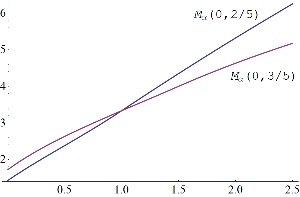
If we take an specific value for $\lambda$ , say $\lambda=1$ , we get $M_{\alpha}(0,2/5)=M_{\alpha}(0,3/5)=10/3$ , and so it is more convenient to take $[\hat{a},\hat{b}]=[0,2/5]$ . The reason for this is that $f_{\rho,\rho/c}(0,2/5)\geq f_{\rho,\rho/c}(0,3/5)$ independently of $f$ , and so $\mathrm{I}_{\rho}^{0}$ is more easily satisfied.

Observe in Figure 3 that the graphs of $M_{\alpha}(0,2/5)(\lambda)$ and $M_{\alpha}(0,3/5)(\lambda)$ cross at $\lambda=1$ . If $f$ is continuous and $f_{\rho,\rho/c}(0,2/5)>f_{\rho,\rho/c}(0,3/5)$ , since $M_{\alpha}(0,2/5)(1)$ is a better choice than $M_{\alpha}(0,3/5)(1)$ , by the continuity of $f$ , so it will be in a neighborhood of $1$ . That shows that the condition $M_{\alpha}(0,2/5)(\lambda)<M_{\alpha}(0,3/5)(\lambda)$ may help but is not deciding when choosing the interval.

Acknowledgements

The authors want to express their gratitude towards the physicist Santiago Codesido, whose ideas helped develop the model in Section 4.1. This paper was partially written during a visit of G. Infante to the Departamento de Análise Matemática of the Universidade de Santiago de Compostela. G. Infante is grateful to the people of the aforementioned Departamento for their kind and warm hospitality.

References

[1] A. R. Aftabizadeh, Y. K. Huang and J. Wiener, Bounded solutions for differential equations with reflection of the argument, J. Math. Anal. Appl., 135 (1988), 31–37.
[2] H. Amann, Fixed point equations and nonlinear eigenvalue problems in ordered Banach spaces, SIAM. Rev., 18 (1976), 620–709.
[3] D. Andrade and T. F. Ma, Numerical solutions for a nonlocal equation with reflection of the argument, Neural Parallel Sci. Comput., 10 (2002), 227–233.
[4] M. Brokate and A. Friedman, Optimal design for heat conduction problems with hysteresis, Siam J. Control and Optimization, 27-4 (1989), 697–717.
[5] A. Cabada, The method of lower and upper solutions for third – order periodic boundary value problems. J. Math. Anal. Appl., 195 (1995), 568–589 .
[6] A. Cabada and F. A. F. Tojo, Comparison results for first order linear operators with reflection and periodic boundary value conditions, Nonlinear Anal., 78 (2013), 32–46.
[7] A. Cabada and F. A. F. Tojo, Solutions of the first order linear equation with reflection and general linear conditions, Global Journal of Mathematical Sciences (GJMS), 2:1 (2013).
[8] A. Cabada and F. A. F. Tojo, Existence results for a linear equation with reflection, non-constant coefficient and periodic boundary conditions, J. Math. Anal. Appl., 412 (2013), 529–546.
[9] A. Cabada, G. Infante and F. A. F. Tojo, Nontrivial solutions of perturbed Hammerstein integral equations with reflections, Bound. Value Probl., 2013:86 (2013).
[10] A. Cabada, R. L. Pouso and F.L. Minhós, Extremal solutions to fourth-order functional boundary value problems including multipoint conditions, Nonlinear Anal. Real World Appl., 10 (2009), 2157–2170.
[11] S. Campbell and J. W. Macki, Control of the temperature at one end of a rod, Math. Comput. Modelling, 32 (2000), 825–842.
[12] W. W. Coblentz, Emissivity of straight and helical filaments of tungsten, Bulletin of the Bureau of Standards, 14 (1918), 115–131.
[13] R. Conti, Recent trends in the theory of boundary value problems for ordinary differential equations. Boll. Un. Mat. Ital., 22 (1967), 135–178.
[14] H. Fan and R. Ma, Loss of positivity in a nonlinear second order ordinary differential equations, Nonlinear Anal., 71 (2009), 437–444.
[15] R. Figueroa and R. L. Pouso, Minimal and maximal solutions to second-order boundary value problems with state-dependent deviating arguments, Bull. Lond. Math. Soc., 43 (2011), 164–174.
[16] A. Friedman and L. S. Jiang, Periodic solutions for a thermostat control problem, Comm. in Partial Differential Equations, 13 (1988), 515–550.
[17] D. Franco, G. Infante and D. O’Regan, Positive and nontrivial solutions for the Urysohn integral equation, Acta Math. Sin., 22 (2006), 1745–1750.
[18] D. Franco, G. Infante and D. O’Regan, Nontrivial solutions in abstract cones for Hammerstein integral systems, Dyn. Contin. Discrete Impuls. Syst. Ser. A Math. Anal., 14 (2007), 837–850.
[19] C. S. Goodrich, On nonlinear boundary conditions satisfying certain asymptotic behavior, Nonlinear Anal., 76 (2013), 58–67.
[20] P. Guidotti and S. Merino, Gradual loss of positivity and hidden invariant cones in a scalar heat equation, Differential Integral Equations, 13 (2000), 1551–1568.
[21] D. Guo and V. Lakshmikantham, Nonlinear Problems in Abstract Cones, Academic Press, 1988.
[22] Ch. P. Gupta, Existence and uniqueness theorems for boundary value problems involving reflection of the argument, Nonlinear Anal., 11 (1987), 1075–1083.
[23] Ch. P. Gupta, Two-point boundary value problems involving reflection of the argument, Internat. J. Math. Math. Sci., 10 (1987), 361–371.
[24] G. Infante, Eigenvalues of some non-local boundary-value problems, Proc. Edinb. Math. Soc., 46 (2003), 75–86.
[25] G. Infante, Positive solutions of some nonlinear BVPs involving singularities and integral BCs, Discrete Contin. Dyn. Syst. Series S, 1 (2008), 99–106.
[26] G. Infante, Nonlocal boundary value problems with two nonlinear boundary conditions, Commun. Appl. Anal., 12 (2008), 279–288.
[27] G. Infante and P. Pietramala, Nonlocal impulsive boundary value problems with solutions that change sign, CP1124, Mathematical Models in Engineering, Biology, and Medicine, Proceedings of the International Conference on Boundary Value Problems, edited by A. Cabada, E. Liz, and J.J. Nieto, (2009), 205–213.
[28] G. Infante and P. Pietramala, Perturbed Hammerstein integral inclusions with solutions that change sign, Comment. Math. Univ. Carolin., 50 (2009), 591–605.
[29] G. Infante and P. Pietramala, A cantilever equation with nonlinear boundary conditions Electron. J. Qual. Theory Differ. Equ., Spec. Ed. I, No. 15 (2009), 1–14.
[30] G. Infante and J. R. L. Webb, Three point boundary value problems with solutions that change sign, J. Integral Equations Appl., 15, (2003), 37–57.
[31] G. Infante and J. R. L. Webb, Nonzero solutions of Hammerstein integral equations with discontinuous kernels, J. Math. Anal. Appl., 272 (2002), 30–42.
[32] G. Infante and J. R. L. Webb, Loss of positivity in a nonlinear scalar heat equation, NoDEA Nonlinear Differential Equations Appl., 13 (2006), 249–261.
[33] G. Infante and J. R. L. Webb, Nonlinear nonlocal boundary value problems and perturbed Hammerstein integral equations, Proc. Edinb. Math. Soc., 49 (2006), 637–656.
[34] T. Jankowski, Solvability of three point boundary value problems for second order differential equations with deviating arguments, J. Math. Anal. Appl., 312 (2005), 620–636.
[35] T. Jankowski, Multiple solutions for a class of boundary-value problems with deviating arguments and integral boundary conditions, Dynam. Systems Appl., 19 (2010), 179–188.
[36] T. Jankowski, Nonnegative solutions to nonlocal boundary value problems for systems of second-order differential equations dependent on the first-order derivatives, Nonlinear Anal., 87 (2013), 83–101.
[37] T. Jankowski, Positive solutions to second-order differential equations with dependence on the first-order derivative and nonlocal boundary conditions, Bound. Value Probl., 2013:8 (2013).
[38] T. Jankowski, Positive solutions to Sturm-Liouville problems with nonlocal boundary conditions, Proc. Roy. Soc. Edinburgh Sect. A, 144A (2014), 119–138.
[39] T. Jankowski and W. Szatanik, Second-order differential equations with deviating arguments, Bound. Value Probl. 2006, Art. ID 23092, 15 pp.
[40] G. L. Karakostas and P. Ch. Tsamatos, Existence of multiple positive solutions for a nonlocal boundary value problem, Topol. Methods Nonlinear Anal., 19 (2002), 109–121.
[41] G. L. Karakostas and P. Ch. Tsamatos, Multiple positive solutions of some Fredholm integral equations arisen from nonlocal boundary-value problems, Electron. J. Differential Equations, 2002, No. 30, 17 pp.
[42] I. Karatsompanis and P. K. Palamides, Polynomial approximation to a non-local boundary value problem, Comput. Math. Appl., 60 (2010), 3058–3071.
[43] M. A. Krasnosel’skiĭ and P. P. Zabreĭko, Geometrical methods of nonlinear analysis, Springer-Verlag, Berlin, (1984).
[44] K. Q. Lan, Multiple positive solutions of Hammerstein integral equations with singularities, Differential Equations and Dynamical Systems, 8 (2000), 175–195.
[45] T. F. Ma, E. S. Miranda and M. B. de Souza Cortes, A nonlinear differential equation involving reflection of the argument, Arch. Math. (Brno), 40 (2004), 63–68.
[46] R. Ma, A survey on nonlocal boundary value problems, Appl. Math. E-Notes, 7 (2001), 257–279.
[47] R. H. Martin, Nonlinear operators and differential equations in Banach spaces, Wiley, New York, (1976).
[48] J. J. Nieto and J. Pimentel, Positive solutions of a fractional thermostat model, Bound. Value Probl., 2013:5 (2013).
[49] S. K. Ntouyas, Nonlocal initial and boundary value problems: a survey, Handbook of differential equations: ordinary differential equations. Vol. II, 461–557, Elsevier B. V., Amsterdam, 2005.
[50] P. Pietramala, A note on a beam equation with nonlinear boundary conditions, Bound. Value Probl., (2011), Art. ID 376782, 14 pp.
[51] M. Picone, Su un problema al contorno nelle equazioni differenziali lineari ordinarie del secondo ordine, Ann. Scuola Norm. Sup. Pisa Cl. Sci., 10 (1908), 1–95.
[52] D. O’Regan, Existence results for differential equations with reflection of the argument, J. Austral. Math. Soc. Ser. A, 57 (1994), 237–260.
[53] D. O’Regan and M. Zima, Leggett-Williams norm-type fixed point theorems for multivalued mappings, Appl. Math. Comput., 187 (2007), 1238–1249.
[54] P. K. Palamides, G. Infante and P. Pietramala, Nontrivial solutions of a nonlinear heat flow problem via Sperner’s lemma, Appl. Math. Lett., 22 (2009), 1444–1450.
[55] D. Piao, Pseudo almost periodic solutions for differential equations involving reflection of the argument, J. Korean Math. Soc., 41 (2004), 747–754.
[56] D. Piao, Periodic and almost periodic solutions for differential equations with reflection of the argument, Nonlinear Anal., 57 (2004), 633–637.
[57] D. Piao, Bounded and almost periodic solutions for second order differential equation involving reflection of the argument, arXiv:1302.0616.
[58] A. Štikonas, A survey on stationary problems, Green’s functions and spectrum of Sturm-Liouville problem with nonlocal boundary conditions, Nonlinear Anal. Model. Control, 19 (2014), 301–334.
[59] W. Szatanik, Quasi-solutions for generalized second order differential equations with deviating arguments, J. Comput. Appl. Math., 216 (2008), 425–434.
[60] W. Szatanik, Minimal and maximal solutions for integral boundary value problems for the second order differential equations with deviating arguments, Dynam. Systems Appl., 19 (2010), 87–96.
[61] P. J. Torres, Existence of one-signed periodic solutions of some second-order differential equations via a Krasnoselskii fixed point theorem, J. Differential Equations, 190 (2003), 643–662.
[62] K. Ujihara, Reflectivity of metals at high temperatures, J. Appl. Phys., 43 (1972), 2376–2383.
[63] J. R. L. Webb, Multiple positive solutions of some nonlinear heat flow problems, Discrete Contin. Dyn. Syst., suppl. (2005), 895–903.
[64] J. R. L. Webb, Optimal constants in a nonlocal boundary value problem, Nonlinear Anal., 63 (2005), 672–685.
[65] J. R. L. Webb, Existence of positive solutions for a thermostat model, Nonlinear Anal. Real World Appl., 13 (2012), 923–938
[66] J. R. L. Webb and G. Infante, Positive solutions of nonlocal boundary value problems: a unified approach, J. London Math. Soc., 74 (2006), 673–693.
[67] J. R. L. Webb and G. Infante, Positive solutions of nonlocal boundary value problems involving integral conditions, NoDEA Nonlinear Differential Equations Appl., 15 (2008), 45–67.
[68] J. R. L. Webb and G. Infante, Nonlocal boundary value problems of arbitrary order, J. London Math. Soc., 79 (2009), 238–258.
[69] J. R. L. Webb and M. Zima, Multiple positive solutions of resonant and non-resonant nonlocal boundary value problems, Nonlinear Anal., 71 (2009), 1369–1378.
[70] W. M. Whyburn, Differential equations with general boundary conditions, Bull. Amer. Math. Soc., 48 (1942), 692–704.
[71] J. Wiener and A. R. Aftabizadeh, Boundary value problems for differential equations with reflection of the argument, Internat. J. Math. Math. Sci., 8 (1985), 151–163.