Solving Relational MDPs with Exogenous Events and Additive Rewards
Abstract
We formalize a simple but natural subclass of service domains for relational planning problems with object-centered, independent exogenous events and additive rewards capturing, for example, problems in inventory control. Focusing on this subclass, we present a new symbolic planning algorithm which is the first algorithm that has explicit performance guarantees for relational MDPs with exogenous events. In particular, under some technical conditions, our planning algorithm provides a monotonic lower bound on the optimal value function. To support this algorithm we present novel evaluation and reduction techniques for generalized first order decision diagrams, a knowledge representation for real-valued functions over relational world states. Our planning algorithm uses a set of focus states, which serves as a training set, to simplify and approximate the symbolic solution, and can thus be seen to perform learning for planning. A preliminary experimental evaluation demonstrates the validity of our approach.
1 Introduction
Relational Markov Decision Processes (RMDPs) offer an attractive formalism to study both reinforcement learning and probabilistic planning in relational domains. However, most work on RMDPs has focused on planning and learning when the only transitions in the world are a result of the agent’s actions. We are interested in a class of problems modeled as service domains, where the world is affected by exogenous service requests in addition to the agent’s actions. In this paper we use the inventory control (IC) domain as a motivating running example and for experimental validation. The domain models a retail company faced with the task of maintaining the inventory in its shops to meet consumer demand. Exogenous events (service requests) correspond to arrival of customers at shops and, at any point in time, any number of service requests can occur independently of each other and independently of the agent’s action. Although we focus on IC, independent exogenous service requests are common in many other problems, for example, in fire and emergency response, air traffic control, and service centers such as taxicab companies, hospitals, and restaurants. Exogenous events present a challenge for planning and reinforcement learning algorithms because the number of possible next states, the “stochastic branching factor”, grows exponentially in the number of possible simultaneous service requests.
In this paper we consider symbolic dynamic programming (SDP) to solve RMDPs, as it allows to reason more abstractly than what is typical in forward planning and reinforcement learning. The SDP solutions for propositional MDPs can be adapted to RMDPs by grounding the RMDP for each size to get a propositional encoding, and then using a “factored approach” to solve the resulting planning problem, e.g., using algebraic decision diagrams (ADDs) [5] or linear function approximation [4]. This approach can easily model exogenous events [2] but it plans for a fixed domain size and requires increased time and space due to the grounding. The relational (first order logic) SDP approach [3] provides a solution which is independent of the domain size, i.e., it holds for any problem instance. On the other hand, exogenous events make the first order formulation much more complex. To our knowledge, the only work to have approached this is [17, 15]. While Sanner’s work is very ambitious in that it attempted to solve a very general class of problems, the solution used linear function approximation, approximate policy iteration, and some heuristic logical simplification steps to demonstrate that some problems can be solved and it is not clear when the combination of ideas in that work is applicable, both in terms of the algorithmic approximations and in terms of the symbolic simplification algorithms.
In this paper we make a different compromise by constraining the class of problems and aiming for a complete symbolic solution. In particular, we introduce the class of service domains, that have a simple form of independent object-focused exogenous events, so that the transition in each step can be modeled as first taking the agent’s action, and then following a sequence of “exogenous actions” in any order. We then investigate a relational SDP approach to solve such problems. The main contribution of this paper is a new symbolic algorithm that is proved to provide a lower bound approximation on the true value function for service domains under certain technical assumptions. While the assumptions are somewhat strong, they allow us to provide the first complete analysis of relational SDP with exogenous events which is important for understanding such problems. In addition, while the assumptions are needed for the analysis, they are not needed for the algorithm that can be applied in more general settings. Our second main contribution provides algorithmic support to implement this algorithm using the GFODD representation of [8]. GFODDs provide a scheme for capturing and manipulating functions over relational structures. Previous work has analyzed some theoretical properties of this representation but did not provide practical algorithms. In this paper we develop a model evaluation algorithm for GFODDs inspired by variable elimination (VE), and a model checking reduction for GFODDs. These are crucial for efficient realization of the new approximate SDP algorithm. We illustrate the new algorithm in two variants of the IC domain, where one satisfies our assumptions and the other does not. Our results demonstrate that the new algorithm can be implemented efficiently, that its size-independent solution scales much better than propositional approaches [5, 19], and that it produces high quality policies.
2 Preliminaries: Relational Symbolic Dynamic Programming
We assume familiarity with basic notions of Markov Decision Processes (MDPs) and First Order Logic [14, 13]. Briefly, a MDP is given by a set of states , actions , transition function , immediate reward function and discount factor . The solution of a MDP is a policy that maximizes the expected discounted total reward obtained by following that policy starting from any state. The Value Iteration algorithm (VI), calculates the optimal value function by iteratively performing Bellman backups defined for each state as,
| (1) |
Relational MDPs: Relational MDPs are simply MDPs where the states and actions are described in a function-free first order logical language. In particular, the language allows a set of logical constants, a set of logical variables, a set of predicates (each with its associated arity), but no functions of arity greater than 0. A state corresponds to an interpretation in first order logic (we focus on finite interpretations) which specifies (1) a finite set of domain elements also known as objects, (2) a mapping of constants to domain elements, and (3) the truth values of all the predicates over tuples of domain elements of appropriate size (to match the arity of the predicate). Atoms are predicates applied to appropriate tuples of arguments. An atom is said to be ground when all its arguments are constants or domain elements. For example, using this notation is an atom and is a ground atom involving the predicate and object (expressing that the shop is empty in the IC domain). Our notation does not distinguish constants and variables as this will be clear from the context. One of the advantages of relational SDP algorithms, including the one in this paper, is that the number of objects is not known or used at planning time and the resulting policies generalize across domain sizes.
The state transitions induced by agent actions are modeled exactly as in previous SDP work [3]. The agent has a set of action types each parametrized with a tuple of objects to yield an action template and a concrete ground action (e.g. template and concrete action ). To simplify notation, we use to refer to a single variable or a tuple of variables of the appropriate arity. Each agent action has a finite number of action variants (e.g., action success vs. action failure), and when the user performs in state one of the variants is chosen randomly using the state-dependent action choice distribution .
Similar to previous work we model the reward as some additive function over the domain. To avoid some technical complications, we use average instead of sum in the reward function; this yields the same result up to a multiplicative factor.
Relational Expressions and GFODDs: To implement planning algorithms for relational MDPs we require a symbolic representation of functions to compactly describe the rewards, transitions, and eventually value functions. In this paper we use the GFODD representation of [8] but the same ideas work for any representation that can express open-expressions and closed expressions over interpretations (states). An expression represents a function mapping interpretations to real values. An open expression , similar to an open formula in first order logic, can be evaluated in interpretation once we substitute the variables with concrete objects in . A closed expression , much like a closed first order logic formula, aggregates the value of over all possible substitutions of to objects in . First order logic limits to have values in (i.e., evaluate to false or true) and provides the aggregation (corresponding to existential quantification) and (corresponding to universal quantification) that can be used individually on each variable in . Expressions are more general allowing for additional aggregation functions (for example, average) so that aggregation generalizes quantification in logic, and allowing to take numerical values. On the other hand, our expressions require aggregation operators to be at the front of the formulas and thus correspond to logical expressions in prenex normal form. This enables us to treat the aggregation portion and formula portion separately in our algorithms. In this paper we focus on average and max aggregation. For example, in the IC domain we might use the expression: “ (if then 1, else if then 0.1, else 0)”. Intuitively, this awards a 1 for any non-empty shop and at most one shop is awarded a 0.1 if there is a truck at that shop. The value of this expression is given by picking one which maximizes the average over .
GFODDs provide a graphical representation and associated algorithms to represent open and closed expressions. A GFODD is given by an aggregation function, exactly as in the expressions, and a labeled directed acyclic graph that represents the open formula portion of the expression. Each leaf in the GFODD is labeled with a non-negative numerical value, and each internal node is labeled with a first-order atom (allowing for equality atoms) where we allow atoms to use constants or variables as arguments. As in propositional diagrams [1], for efficiency reasons, the order over nodes in the diagram must conform to a fixed ordering over node labels, which are first order atoms in our case. Figure 1(a) shows an example GFODD capturing the expression given in the previous paragraph.
Given a diagram , an interpretation , and a substitution of variables in to objects in , one can traverse a path to a leaf which gives the value for that substitution. The values of all substitutions are aggregated exactly as in expressions. In particular, let the variables as ordered in the aggregation function be . To calculate the final value, , the semantics prescribes that we enumerate all substitutions of variables to objects in and then perform the aggregation over the variables, going from to . We can therefore think of the aggregation as if it organizes the substitutions into blocks (with fixed value to the first variables and all values for the ’th variable), and then aggregates the value of each block separately, repeating this from to . We call the algorithm that follows this definition directly brute force evaluation. A detailed example is shown in Figure 3(a). To evaluate the diagram in Figure 3(a) on the interpretation shown there we enumerate all substitutions of 3 objects to 3 variables, obtain a value for each, and then aggregate the values. In the block where , , and varies over we get the values and an aggregated value of . This can be done for every block, and then we can aggregate over substitutions of and . The final value in this case is .
Any binary operation over real values can be generalized to open and closed expressions in a natural way. If and are two closed expressions, represents the function which maps each interpretation to . We follow the general convention of using and to denote and respectively when they are applied to expressions. This provides a definition but not an implementation of binary operations over expressions. The work in [8] showed that if the binary operation is safe, i.e., it distributes with respect to all aggregation operators, then there is a simple algorithm (the Apply procedure) implementing the binary operation over expressions. For example is safe w.r.t. aggregation, and it is easy to see that = , and the open formula portion (diagram portion) of the result can be calculated directly from the open expressions and . The Apply procedure [20, 8] calculates a diagram representing using operations over the graphs representing and . Note that we need to standardize apart, as in the renaming of to for such operations.

SDP for Relational MDPs: SDP provides a symbolic implementation of the value iteration update of Eq (1) that avoids state enumeration implicit in that equation. The SDP algorithm of [8] generalizing [3] calculates one iteration of value iteration as follows. As input we get (as GFODDs) closed expressions , (we use Figure 1(a) as the reward in the example below), and open expressions for the probabilistic choice of actions and for the dynamics of deterministic action variants.
The action dynamics are specified by providing a diagram (called truth value diagram or TVD) for each variant and predicate template . The corresponding TVD, , is an open expression that specifies the truth value of in the next state when has been executed in the current state. Figure 1(b) shows the TVD of for predicates . Note that in contrast to other representations of planning operators (but similar to the successor state axioms of [3]) TVDs specify the truth value after the action and not the change in truth value. Since unload is deterministic we have only one variant and . We illustrate probabilistic actions in the next section. Following [20, 8] we require that and have no aggregations and cannot introduce new variables, that is, the first refers to only and the second to and but no other variables. This implies that the regression and product terms in the algorithm below do not change the aggregation function and therefore enables the analysis of the algorithm.
The SDP algorithm of [8] implements Eq (1) using the following 4 steps. We denote this as .
- 1.
Regression: The step-to-go value function is regressed over every deterministic variant of every action to produce . Regression is conceptually similar to goal regression in deterministic planning but it needs to be done for all (potentially exponential number of) paths in the diagram, each of which can be thought of as a goal in the planning context. This can be done efficiently by replacing every atom in the open formula portion of (a node in the GFODD representation) by its corresponding TVD without changing the aggregation function.
Figure 1(c) illustrates the process of block replacement for the diagram of part (a). Note that is not affected by the action. Therefore its TVDs simply repeats the predicate value, and the corresponding node is unchanged by block replacement. Therefore, in this example, we are effectively replacing only one node with its TVD. The TVD leaf valued 1 is connected to the left child (true branch) of the node and the 0 leaf is connected to the right child (false branch). To maintain the diagrams sorted we must in fact use a different implementation than block replacement; the implementation does not affect the constructions or proofs in the paper and we therefore refer the reader to [20] for the details.
- 2.
Add Action Variants: The Q-function for each action is generated by combining regressed diagrams using the binary operations and over expressions.
Recall that probability diagrams do not refer to additional variables. The multiplication can therefore be done directly on the open formulas without changing the aggregation function. As argued by [20], to guarantee correctness, both summation steps ( and steps) must standardize apart the functions before adding them.
- 3.
Object Maximization: Maximize over the action parameters to produce for each action , thus obtaining the value achievable by the best ground instantiation of in each state. This step is implemented by converting action parameters in to variables, each associated with the aggregation operator, and appending these operators to the head of the aggregation function.
For example, if object maximization were applied to the diagram of Figure 1(c) (we skipped some intermediate steps) then would be replaced with variables and given max aggregation so that the aggregation is as shown in part (d) of the figure. Therefore, in step 2, are constants (temporarily added to the logical language) referring to concrete objects in the world, and in step 3 we turn them into variables and specify the aggregation function for them.
- 4.
Maximize over Actions: The step-to-go value function , is generated by combining the diagrams using the binary operation over expressions.
The main advantage of this approach is that the regression operation, and the binary operations over expressions , , can be performed symbolically and therefore the final value function output by the algorithm is a closed expression in the same language. We therefore get a completely symbolic form of value iteration. Several instantiations of this idea have been implemented [11, 6, 18, 20]. Except for the work of [8, 18] previous work has handled only max aggregation. Previous work [8] relies on the fact that the binary operations , , and are safe with respect to aggregation to provide a GFODD based SDP algorithm for problems where the reward function has and aggregations . In this paper we use reward functions with and avg aggregation. The binary operations and are safe with respect to avg but the binary operation is not. For example but . To address this issue we introduce a new implementation for this case in the next section.
3 Model and Algorithms for Service Domains
We now proceed to describe our extensions to SDP to handle exogenous events. Exogenous events refer to spontaneous changes to the state without agent action. Our main modeling assumption, denoted A1, is that we have object-centered exogenous actions that are automatically taken in every time step. In particular, for every object in the domain we have action that acts on object and the conditions and effects of are such that they are mutually non-interfering: given any state , all the actions are applied simultaneously, and this is equivalent to their sequential application in any order. We use the same GFODD action representation described in the previous section to capture the dynamics of .
Example: IC Domain. We use a simple version of the inventory control domain (IC) as a running example, and for some of the experimental results. In IC the objects are a depot, a truck and a number of shops. A shop can be empty or full, i.e., the inventory has only two levels and the truck can either be at the depot or at a shop. The reward is the fraction (average) of non-empty shops. Agent actions are deterministic and they capture stock replacement. In particular, a shop can be filled by unloading inventory from the truck in one step. The truck can be loaded in a depot and driven from any location (shop or depot) to any location in one step. The exogenous action has two variants; the success variant (customer arrives at shop , and if non-empty the inventory becomes empty) occurs with probability 0.4 and the fail variant (no customer, no changes to state) occurs with probability 0.6. Figure 2 parts (a)-(d) illustrate the model for IC and its GFODD representation. In order to facilitate the presentation of algorithmic steps, Figure 2(e) shows a slightly different reward function (continuing previous examples) that is used as the reward in our running example.
For our analysis we make two further modeling assumptions. A2: we assume that exogenous action can only affect unary properties of the object . To simplify the presentation we consider a single such predicate that may be affected, but any number of such predicates can be handled. In IC, the special predicate is specifying whether the shop is empty. A3: we assume that does not appear in the precondition of any agent action. It follows that only affects and that can appear in the precondition of but cannot appear in the precondition of any other action.
3.1 The Template Method

Extending SDP to handle exogenous events is complicated because the events depend on the objects in the domain and on their number and exact solutions can result in complex expressions that require counting formulas over the domain [17, 15]. A possible simple approach would explicitly calculate the composition of the agent’s actions with all the exogenous events. But this assumes that we know the number of objects (and thus does not generalize) and results in an exponential number of action variants, which makes it infeasible. A second simple approach would be to directly modify the SDP algorithm so that it sequentially regresses the value function over each of the ground exogenous actions before performing the regression over the agent actions, which is correct by our assumptions. However, this approach, too, requires us to know and because it effectively grounds the solution it suffers in terms of generality.
We next describe the template method, one of our main contributions, which provides a completely abstract approximate SDP solution for the exogenous event model. We make our final assumption, A4, that the reward function (and inductively ) is a closed expression of the form where is a (potentially empty) set of variables and is a single variable, and in the predicate appears instantiated only as . The IC domain as described above satisfies all our assumptions.
The template method first runs the following 4 steps, denoted , and then follows with the 4 steps of SDP as given above for user actions. The final output of our approximate Bellman backup, , is .
1. Grounding:
Let be a Skolem constant
not in .
Partially ground to get
2. Regression: The function is
regressed over every deterministic variant of the exogenous
action centered at to produce .
3. Add Action Variants: The value function
is updated.
As in , multiplication is done directly on the open formulas
without changing the aggregation function.
Importantly, in contrast with ,
here we do not
standardize apart the functions when performing . This leads to an
approximation.
4. Lifting:
Let the output of the previous step be
.
Return .
Thus, the algorithm grounds using a generic object for exogenous actions, it then performs regression for a single generic exogenous action, and then reintroduces the aggregation. Figure 2 parts (e)-(j) illustrate this process.
We now show that our algorithm provides a monotonic lower bound on the value function. The crucial step is the analysis of . We have:
Lemma 1
Under assumptions A1, A2, A4 the value function calculated by is a lower bound on the value of regression of through all exogenous actions.
Due to space constraints the complete proof is omitted and we only provide a sketch. This proof and other omitted details can be found in the full version of this paper [10].
Proof
(sketch) The main idea in the proof is to show that, under our assumptions, the result of our algorithm is equivalent to sequential regression of all exogenous actions, where in each step the action variants are not standardized apart.
Recall that the input value function has the form . To establish this relationship we show that after the sequential algorithm regresses the intermediate value function has the form . That is, the first portions change in the same structural manner into a diagram and the remaining portions retain their original form . In addition, is the result of regressing through which is the same form as calculated by step 3 of the template method. Therefore, when all have been regressed, the result is which is the same as the result of the template method.
The sequential algorithm is correct by definition when standardizing apart but yields a lower bound when not standardizing apart. This is true because for any functions and we have where the last equality holds because and range over the same set of objects. Therefore, if and are the results of regression for different variants from step 2, adding them without standardizing apart as in the last equation yields a lower bound. ∎
The lemma requires that used as input satisfies A4. If this holds for the reward function, and if maintains this property then A4 holds inductively for all . Put together this implies that the template method provides a lower bound on the true Bellman backup. It therefore remains to show how can be implemented for aggregation and that it maintains the form A4.
First consider regression. If assumption A3 holds, then our algorithm using regression through TVDs does not introduce new occurrences of into . Regression also does not change the aggregation function. Similarly, the probability diagrams do not introduce and do not change the aggregation function. Therefore A4 is maintained by these steps. For the other steps we need to discuss the binary operations and .
For , using the same argument as above, we see that and therefore it suffices to standardize apart the portion but can be left intact and A4 is maintained.
Finally, recall that we need a new implementation for the binary operation with avg aggregation. This can be done as follows: to perform we can introduce two new variables and write the expression: “ (if then else )”. This is clearly correct whenever the interpretation has at least two objects because are unconstrained. Now, because the branches of the if statement are mutually exclusive, this expression can be further simplified to “ (if then else )”. The implementation uses an equality node at the root with label , and hangs and at the true and false branches. Crucially it does not need to standardize apart the representation of and and thus A4 is maintained. This establishes that the approximation returned by our algorithm, , is a lower bound of the true Bellman backup .
An additional argument (details available in [10]) shows that this is a monotonic lower bound, that is, for all we have where is the true Bellman backup. It is well known (e.g., [12]) that if this holds then the value of the greedy policy w.r.t. is at least (this follows from the monotonicity of the policy update operator ). The significance is, therefore, that provides an immediate certificate on the quality of the resulting greedy policy. Recall that is our approximate backup, and . We have:
Theorem 3.1
When assumptions A1, A2, A3, A4 hold and the reward function is non-negative we have for all : .
As mentioned above, although the assumptions are required for our analysis, the algorithm can be applied more widely. Assumptions A1 and A4 provide our basic modeling assumption per object centered exogenous events and additive rewards. It is easy to generalize the algorithm to have events and rewards based on object tuples instead of single objects. Similarly, while the proof fails when A2 (exogenous events only affect special unary predicates) is violated the algorithm can be applied directly without modification. When A3 does not hold, can appear with multiple arguments and the algorithm needs to be modified. Our implementation introduces an additional approximation and at iteration boundary we unify all the arguments of with the average variable . In this way the algorithm can be applied inductively for all . These extensions of the algorithm are demonstrated in our experiments.
Relation to Straight Line Plans: The template method provides symbolic way to calculate a lower bound on the value function. It is interesting to consider what kind of lower bound this provides. Recall that the straight line plan approximation (see e.g., discussion in [2]) does not calculate a policy and instead at any state it seeks the best linear plan with highest expected reward. As the next observation argues (proof available in [10]) the template method provides a related approximation. We note, however, that unlike previous work on straight line plans our computation is done symbolically and calculates the approximation for all start states simultaneously.
Observation 1
The template method provides an approximation that is related to the value of the best straight line plan. When there is only one deterministic agent action template we get exactly the value of the straight line plan. Otherwise, the approximation is bounded between the value of the straight line plan and the optimal value.
4 Evaluation and Reduction of GFODDs
The symbolic operations in the SDP algorithm yield diagrams that are redundant in the sense that portions of them can be removed without changing the values they compute. Recently, [8, 7] introduced the idea of model checking reductions to compress such diagrams. The basic idea is simple. Given a set of “focus states” , we evaluate the diagram on every interpretation in . Any portion of the diagram that does not “contribute” to the final value in any of the interpretations is removed. The result is a diagram which is exact on the focus states, but may be approximate on other states. We refer the reader to [8, 7] for further motivation and justification. In that work, several variants of this idea have been analyzed formally (for and aggregation), have been shown to perform well empirically (for aggregation), and methods for generating via random walks have been developed. In this section we develop the second contribution of the paper, providing an efficient realization of this idea for aggregation.
The basic reduction algorithm, which we refer to below as brute force model checking for GFODDs, is: (1) Evaluate the diagram on each example in our focus set marking all edges that actively participate in generating the final value returned for that example. Because we have this value is given by the “winner” of max aggregation. This is a block of substitutions that includes one assignment to and all possible assignments to . For each such block collect the set of edges traversed by any of the substitutions in the block. When picking the max block, also collect the edges traversed by that block, breaking ties by lexicographic ordering over edge sets. (2) Take the union of marked edges over all examples, connecting any edge not in this set to 0.

Consider again the example of evaluation in Figure 3(a), where we assigned node identifiers 1,2,3. We identify edges by their parent node and its branch so that the left-going edge from the root is edge . In this case the final value is achieved by multiple blocks of substitutions, and two distinct sets of edges and . Assuming and , is lexicographically smaller and is chosen as the marked set. This process is illustrated in the tables of Figure 3(a). Referring to the reduction procedure, if our focus set includes only this interpretation, then the edges will be redirected to the value 0.
Efficient Model Evaluation and Reduction: We now show that the same process of evaluation and reduction can be implemented more efficiently. The idea, taking inspiration from variable elimination, is that we can aggregate some values early while calculating the tables. However, our problem is more complex than standard variable elimination and we require a recursive computation over the diagram.
For every node let be the literal at the node and let and be its false and true branches respectively. Define to be the set of variables appearing above and to be the variables in . Let and be the variables of largest index in and respectively. Finally let be the maximum between and . Figure 3(b) shows and for our example diagram. Given interpretation , let be the set of bindings of objects from to variables in such that . Similarly is the set of bindings such that . The two sets are obviously disjoint and together cover all bindings for . For example, for the root node in the diagram of Figure 3(b), is a table mapping to and is a table mapping to . The evaluation procedure, Eval(), is as follows:
- 1.
If is a leaf:
(1) Build a “table” with all variables implicit, and with the value of .
(2) Aggregate over all variables from the last variable down to .
(3) Return the resulting table. - 2.
Otherwise is an internal node:
(1) Let Eval(), where is the join of the tables.
(2) Aggregate over all the variables in from the last variable not yet aggregated down to .
(3) Let Eval()
(4) Aggregate over all the variables in from the last variable not yet aggregated down to .
(5) Let .
(6) Aggregate over all the variables in from the last variable not yet aggregated down to .
(7) Return node table .
We note several improvements for this algorithm and its application for reductions, all of which are applicable and used in our experiments. (I1) We implement the above recursive code using dynamic programming to avoid redundant calls. (I2) When an aggregation operator is idempotent, i.e., , aggregation over implicit variables does not change the table, and the implementation is simplified. This holds for and avg aggregation. (I3) In the case of aggregation the procedure is made more efficient (and closer to variable elimination where variable order is flexible) by noting that, within the set of variables , aggregation can be done in any order. Therefore, once has been aggregated, any variable that does not appear above node can be aggregated at . (I4) The recursive algorithm can be extended to collect edge sets for winning blocks by associating them with table entries. Leaf nodes have empty edge sets. The join step at each node adds the corresponding edge (for true or false child) for each entry. Finally, when aggregating an average variable we take the union of edges, and when aggregating a max variable we take the edges corresponding to the winning value, breaking ties in favor of the lexicographically smaller set of edges.
A detailed example of the algorithm is given in Figure 3(b) where the evaluation is on the same interpretation as in part (a). We see that node 3 first collects a table over and that, because is not used above, it already aggregates . The join step for node 2 uses entries and for from the left child and other entries from the right child. Node 2 collects the entries and (using I3) aggregates even though appears above. Node 1 then similarly collects and combines the tables and aggregates . The next theorem is proved by induction over the structure of the GFODD (details available in [10]).
Theorem 4.1
The value and max block returned by the modified Eval procedure are identical to the ones returned by the brute force method.




5 Experimental Validation
In this section we present an empirical demonstration of our algorithms. To that end we implemented our algorithms in Prolog as an extension of the FODD-Planner [9], and compared it to SPUDD [5] and MADCAP [19] that take advantage of propositionally factored state spaces, and implement VI using propositional algebraic decision diagrams (ADD) and affine ADDs respectively. For SPUDD and MADCAP, the domains were specified in the Relational Domain Description Language (RDDL) and translated into propositional descriptions using software provided for the IPPC 2011 planning competition [16]. All experiments were run on an Intel Core 2 Quad CPU @ 2.83GHz. Our system was given Gb of memory and SPUDD and MADCAP were given Gb.
We tested all three systems on the IC domain as described above where shops and trucks have binary inventory levels (empty or full). We present results for the IC domain, because it satisfies all our assumptions and because the propositional systems fare better in this case. We also present results for a more complex IC domain (advanced IC or AIC below) where the inventory can be in one of levels 0,1 and 2 and a shop can have one of consumption rates and . AIC does not satisfy assumption A3. As the experiments show, even with this small extension, the combinatorics render the propositional approach infeasible. In both cases, we constructed the set of focus states to include all possible states over 2 shops. This provides exact reduction for states with 2 shops but the reduction is approximate for larger states as in our experiments.
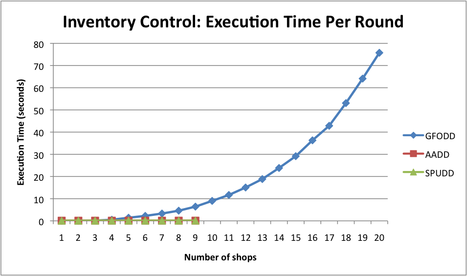
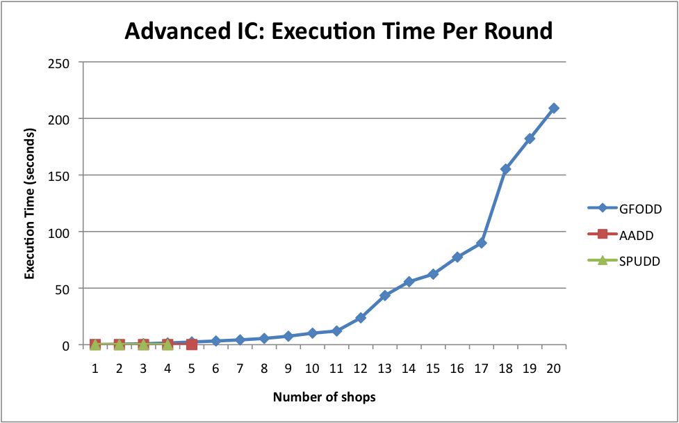
Figure 4 summarizes our results, which we discuss from left to right and top to bottom. The top left plot shows runtime as a function of iterations for AIC and illustrates that the variable elimination method is significantly faster than brute force evaluation and that it enables us to run many more iterations. The top right plot shows the total time (translation from RDDL to a propositional description and off-line planning for 10 iterations of VI) for the 3 systems for one problem instance per size for AIC. SPUDD runs out of memory and fails on more than 4 shops and MADCAP can handle at most 5 shops. Our planning time (being domain size agnostic) is constant. Runtime plots for IC are omitted but they show a similar qualitative picture, where the propositional systems fail with more than shops for SPUDD and shops for MADCAP.
The middle two plots show the cost of using the policies, that is, the on-line execution time as a function of increasing domain size in test instances. To control run time for our policies we show the time for the GFODD policy produced after 4 iterations, which is sufficient to solve any problem in IC and AIC.11 1 Our system does not achieve structural convergence because the reductions are not comprehensive. We give results at 4 iterations as this is sufficient for solving all problems in this domain. With more iterations, our policies are larger and their execution is slower. On-line time for propositional systems is fast for the domain sizes they solve, but our system can solve problems of much larger size (recall that the state space grows exponentially with the number of shops). The bottom two plots show the total discounted reward accumulated by each system (as well as a random policy) on randomly generated problem instances averaged over 30 runs. In both cases all algorithms are significantly better than the random policy. In IC our approximate policy is not distinguishable from the optimal (SPUDD). In AIC the propositional policies are slightly better (differences are statistically significant). In summary, our system provides a non-trivial approximate policy but is sub-optimal in some cases, especially in AIC where A3 is violated. On the other hand its offline planning time is independent of domain size, and it can solve instances that cannot be solved by the propositional systems.
6 Conclusions
The paper presents service domains as an abstraction of planning problems with additive rewards and with multiple simultaneous but independent exogenous events. We provide a new relational SDP algorithm and the first complete analysis of such an algorithm with provable guarantees. In particular our algorithm, the template method, is guaranteed to provide a monotonic lower bound on the true value function under some technical conditions. We have also shown that this lower bound lies between the value of straight line plans and the true value function. As a second contribution we introduce new evaluation and reduction algorithms for the GFODD representation, that in turn facilitate efficient implementation of the SDP algorithm. Preliminary experiments demonstrate the viability of our approach and that our algorithm can be applied even in situations that violate some of the assumptions used in the analysis. The paper provides a first step toward analysis and solutions of general problems with exogenous events by focusing on a well defined subset of such models. Identifying more general conditions for existence of compact solutions, representations for such solutions, and associated algorithms is an important challenge for future work. In addition, the problems involved in evaluation and application of diagrams are computationally demanding. Techniques to speed up these computations are an important challenge for future work.
Acknowledgements
This work was partly supported by NSF under grants IIS-0964457 and IIS-0964705 and the CI fellows award for Saket Joshi. Most of this work was done when Saket Joshi was at Oregon State University.
References
- [1] Bahar, R., Frohm, E., Gaona, C., Hachtel, G., Macii, E., Pardo, A., Somenzi, F.: Algebraic decision diagrams and their applications. In: Proceedings of the IEEE/ACM International Conference on Computer-Aided Design. pp. 188–191 (1993)
- [2] Boutilier, C., Dean, T., Hanks, S.: Decision-theoretic planning: Structural assumptions and computational leverage. Journal of Artificial Intelligence Research 11, 1–94 (1999)
- [3] Boutilier, C., Reiter, R., Price, B.: Symbolic dynamic programming for first-order MDPs. In: Proceedings of the International Joint Conference of Artificial Intelligence. pp. 690–700 (2001)
- [4] Guestrin, C., Koller, D., Parr, R., Venkataraman, S.: Efficient solution algorithms for factored MDPs. Journal of Artificial Intelligence Research 19, 399–468 (2003)
- [5] Hoey, J., St-Aubin, R., Hu, A., Boutilier, C.: SPUDD: Stochastic planning using decision diagrams. In: Proceedings of Uncertainty in Artificial Intelligence. pp. 279–288 (1999)
- [6] Hölldobler, S., Karabaev, E., Skvortsova, O.: FluCaP: a heuristic search planner for first-order MDPs. Journal of Artificial Intelligence Research 27, 419–439 (2006)
- [7] Joshi, S., Kersting, K., Khardon, R.: Self-Taught decision theoretic planning with first-order decision diagrams. In: Proceedings of the International Conference on Automated Planning and Scheduling. pp. 89–96 (2010)
- [8] Joshi, S., Kersting, K., Khardon, R.: Decision theoretic planning with generalized first order decision diagrams. Artificial Intelligence 175, 2198–2222 (2011)
- [9] Joshi, S., Khardon, R.: Probabilistic relational planning with first-order decision diagrams. Journal of Artificial Intelligence Research 41, 231–266 (2011)
- [10] Joshi, S., Khardon, R., Tadepalli, P., Raghavan, A., Fern, A.: Solving relational MDPs with exogenous events and additive rewards. CoRR abs/1306.6302 (2013), http://arxiv.org/abs/1306.6302
- [11] Kersting, K., van Otterlo, M., De Raedt, L.: Bellman goes relational. In: Proceedings of the International Conference on Machine Learning. pp. 465–472 (2004)
- [12] McMahan, H.B., Likhachev, M., Gordon, G.J.: Bounded real-time dynamic programming: RTDP with monotone upper bounds and performance guarantees. In: Proceedings of the International Conference on Machine Learning. pp. 569–576 (2005)
- [13] Puterman, M.L.: Markov Decision Processes: Discrete Stochastic Dynamic Programming. Wiley (1994)
- [14] Russell, S., Norvig, P.: Artificial Intelligence: A Modern Approach. Prentice Hall Series in Artificial Intelligence (2002)
- [15] Sanner, S.: First-order decision-theoretic planning in structured relational environments. Ph.D. thesis, University of Toronto (2008)
- [16] Sanner, S.: Relational dynamic influence diagram language (RDDL): Language description http://users.cecs.anu.edu.au/sanner/IPPC 2011/RDDL.pdf (2010)
- [17] Sanner, S., Boutilier, C.: Approximate solution techniques for factored first-order MDPs. In: Proceedings of the International Conference on Automated Planning and Scheduling. pp. 288–295 (2007)
- [18] Sanner, S., Boutilier, C.: Practical solution techniques for first-order MDPs. Artificial Intelligence 173, 748–788 (2009)
- [19] Sanner, S., Uther, W., Delgado, K.: Approximate dynamic programming with affine ADDs. In: Proceeding of the International Conference on Autonomous Agents and Multiagent Systems. pp. 1349–1356 (2010)
- [20] Wang, C., Joshi, S., Khardon, R.: First-Order decision diagrams for relational MDPs. Journal of Artificial Intelligence Research 31, 431–472 (2008)
Appendix
The appendix provides additional details and proofs that were omitted from the main body of the paper due to space constraints.
7 Proof of Lemma 1 ( Provides a Lower Bound)
In the following we consider performing sequential regression similar to the second simple approach, but where in each step the action variants are not standardized apart. We show that the result of our algorithm, which uses a different computational procedure, is equivalent to this procedure. We then argue that this approach provides a lower bound.
Recall that the input value function has the form which we can represent in explicit expanded form as . Figure 5(a) shows this expanded form of for our running example. To establish this relationship we show that after the sequential algorithm regresses the intermediate value function has the form
| (2) |
as shown in Figure 5(b). That is, the first portions change in the same structural manner into a diagram and the remaining portions retain their original form. In addition, is the result of regressing through which is the same form as calculated by step 3 of the template method. Therefore, when all have been regressed, the result is which is the same as the result of the template method.
We prove the form in Eq (2) by induction over . The base case when no actions have been regressed clearly holds.
We next consider regression of . We use the restriction that regression (via TVDs) does not introduce new variables to conclude that we can regress by regressing each element in the sum separately. Similarly, we use the restriction that probability choice functions do not introduce new variables to conclude that we can push the multiplication into each element of the sum (cf. [18, 8] for similar claims).
Therefore, each action variant produces a function of the form where the superscript indicates regression by the th variant and the form and subscript in indicate that different portions may have changed differently. To be correct, we must standardize apart these functions and add them using the binary operation .
We argue below that (C1) if we do not standardize apart in this step then we get a lower bound on the true value function, and (C2) when we do not standardize apart the result has a special form where only the ’th term is changed and all the terms retain the same value they had before regression. In addition the ’th term changes in a generic way from to . In other words, if we do not standardize apart the action variants of then the result of regression has the form in Eq (2).
It remains to show that C1 and C2 hold. C1 is true because for any functions and we have where the last equality holds because and range over the same set of objects.
For C2 we consider the regression operation and the restriction on the dynamics of exogenous actions. Recall that we allow only unary predicates to be changed by the exogenous actions. To simplify the argument assume that there is only one such predicate . According to the conditions of the proposition can refer to only as . That is, the only argument allowed to be used with is the unique variable for which we have average aggregation.
Now consider the regression of over the explicit sum which is the form guaranteed by the inductive assumption. Because can only change , and because can appear only in , none of the other terms is changed by the regression. This holds for all action variants .
The sequential algorithm next multiplies each element of the sum by the probability of the action variant, and then adds the sums without standardizing apart. Now, when , the ’th term is not changed by regression of . Then for each it is multiplied by and finally all the terms are summed together. This yields exactly the original term ( for and for ). The term does change and this is exactly as in the template method, that is changes to . Therefore C2 holds.

8 Proof of Theorem 3.1 (Monotonic Lower Bound)
The proof of Lemma 1 and the text that follows it imply that for all satisfying A1-A4 we have . Now, when is non-negative, and this implies that for all , we have . We next show that under the same conditions on and we have that for all
| (3) |
Combining the two we get as needed.
We prove Eq (3) by induction on . For the base case it is obvious that because and where is the regressed and discounted value function which is guaranteed to be non-negative.
For the inductive step, note that all the individual operations we use with GFODDs (regress, , , ) are monotonic. That is, consider any functions (GFODDs) such that and then and . As a result, the same is true for any sequence of such operations and in particular for the sequence of operations that defines . Therefore, implies .
9 Proof of Observation 1 (Relation to Straight Line Plans)
The template method provides symbolic way to calculate a lower bound on the value function. It is interesting to consider what kind of lower bound this provides. Consider regression over and the source of approximation in the sequential argument where we do not standardize apart. Treating as the next step value function, captures the ability to take the best action in the next state which is reached after the current exogenous action. Now by calculating the choice of the next action (determined by ) is done without knowledge of which action variant has occurred. Effectively, we have pushed the expectation over action variants into the over actions for the next step. Now, because this is done for all , and at every iteration of the value iteration algorithm, the result is similar to having replaced the true step to go value function
(where is the user action in the ’th step and is the compound exogenous action in the ’th step) with . The last expression is the value of the best linear plan, known as the straight line plan approximation. The analogy given here does not go through completely due to two facts. First, the and expectation are over arguments and not actions. In particular, when there is more than one agent action template (e.g., , ), we explicitly maximize over agent actions in Step 4 of . These max steps are therefore done correctly and are not swapped with expectations. Second, we do still standardize apart agent actions so that their outcomes are taken into consideration. In other words the expectations due to randomization in the outcome of agent actions are performed correctly and are not swapped with max steps. On the other hand, when there is only one agent action template and the action is deterministic we get exactly straight line plan approximation.
10 Preparation for Proof of Theorem 4.1 (Correctness of Model Evaluation Algorithm)
We start by proving the correctness of the evaluation step on its own without the specialization for aggregation and the additional steps for reductions.
The pseudocode for the Eval procedure was given above. Note that the two children of node may have aggregated different sets of variables (due to having additional parents). Therefore in the code we aggregate the table from each side separately (down to ) before taking the union. Once the two sides are combined we still need to aggregate the variables between and before returning the table.
We have the following:
Proposition 1
The value returned by the Eval procedure is exactly .
Proof
Given a node , the value of , and a concrete substitution (for variables to ) reaching in we consider the corresponding block in the brute force evaluation procedure and in our procedure. For the brute force evaluation we fix the values of to to agree with and consider the aggregated value when all variables down to have been aggregated. For Eval() we consider the entry in the table returned by the procedure which is consistent with . Since the table may include some variables (that are smaller than but do not appear below ) implicitly we simply expand the table entry with the values from .
We next prove by induction over the structure of the diagram that the corresponding entries are identical. First, note that if this holds at the root where is the empty set, then the proposition holds because all variables are aggregated and the value is .
For the base case, it is easy to see that the claim holds at a leaf, because all substitutions reaching the leaf have the same value, and the block is explicitly aggregated at the leaf.
Given any node , we have two cases. In the first case, , that is, all variables in are already substituted in . In this case, for any , the entire block traverses (where is either or as appropriate). Clearly, the join with identifies the correct child with respect to the entry of . Consider the table entries in that are extensions of the substitution possibly specifying more variables. More precisely, if the the child node is the entries include the variables up to . By the inductive hypothesis the value in each entry is a correct aggregation of all the variables down to . Now since the remaining variables are explicitly aggregated at , the value calculated at is correct.
In the second case, which means that some extensions of traverse and some traverse . However, as in the previous case, by the inductive hypothesis we know that the extended entries at the children are correct aggregations of their values. Now it is clear that the union operation correctly collects these entries together into one block, and as before because the remaining variables are explicitly aggregated at , the result is correct. ∎
11 Proof of Theorem 4.1 (Correctness of Edge Marking in Model Evaluation Algorithm)
We start by giving a more detailed version of the algorithmic
extension of the algorithm to collect edge sets.
In addition to the the substitution and value,
every table entry is associated with a set of edges.
(1)
When calculating the join we add the edge
to the corresponding table returned by the call to
Eval()
and similarly for and
Eval().
(2)
When a node aggregates an average variable the set of edges for the
new entry is the union of edges in all the entries aggregated.
(3)
When a node aggregates a max variable the set of edges for the
new entry is the set of edges from the winning value. In case of a tie
we pick the set of edges which is smallest lexicographically.
(4) A leaf node returns the empty set as its edge set.
The proof of Theorem 4.1 is similar to the proof above, in that we define a property of nodes and prove it inductively, but in this case it is simpler to argue by way of contradiction.
Proof
The correctness of the value returned was already shown in Proposition 1. We therefore focus on showing that the set of edges returned is identical to the one returned by the brute force method.
For a node and a concrete substitution (for variables to ) reaching in , define to be the sub-diagram of rooted at where to are substituted by , and with the aggregation function of as in where is the last variable in the aggregation function.
We claim that for each node , and that reaches , the entry in the table returned by which is consistent with has the value and set of edges , where is the lexicographically smallest set of edges of a block achieving the value . Note that if the claim holds at the root then the theorem holds because is empty. In the rest of the proof we argue that the set of edges returned is lexicographically smallest.
Now consider any and any and assume by way of contradiction that the claim does not hold for and . Let be the lowest node in for which this happens. That is the claim does hold for all descendants of .
It is easy to see that such a node cannot be a leaf, because for any leaf the set is the empty set and this is what the procedure returns.
For an internal node , again we have two cases. If , then the entire block corresponding to traverses (where as above is or ). In this case, if the last variable (the only one with average aggregation) has not yet been aggregated then the tables are full and the claim clearly holds because aggregation is done directly at node . Otherwise, ’s child aggregated the variables beyond for some . Let be a substitution for . Then by the assumption we know that each entry in the table returned by the child, which is consistent with has value and the lexicographically smallest set of edges corresponding to a block achieving this value.
Now, at node we aggregate using this table. Consider the relevant sub-table with entries where is with the edge added to it by the join operation. Because use aggregation, the aggregation at picks a with the largest value and the corresponding where in case of tie in we pick the entry with smallest .
By our assumption this set is not the lexicographically smallest set corresponding to a block of substitutions realizing the value . Therefore, there must be a block of valuations where is the substitution for realizing the same value and whose edge set is lexicographically smaller than . But in this case for some , and is lexicographically smaller than which (by construction, because the algorithm chose ) is lexicographically smaller than . Thus the entry for is incorrect. This contradicts our assumption that is the lowest node violating the claim.
The second case, where is argued similarly. In this case the substitutions extending may traverse either or . We first aggregate some of the variables in each child’s table. We then take the union of the tables to form the block of (as well as other blocks) and aggregate the remaining . As in the previous case, both of these direct aggregation steps preserve the minimality of the corresponding sets ∎