Generalized Universality of Definite Rank Gluon Transverse Momentum Dependent Correlators

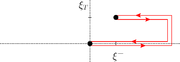
The first type of operator structures contains one color trace and therefore has the simplest gauge link structure that is possible for gluon correlators. This color trace contains both the gluon field operators $F(0)$ and $F(\xi)$ with gauge links running between these two fields and appears when the color in a diagram contributing to the full amplitude flows in just a single color loop. Examples of processes containing such a color structure are processes with colorless particles in the final state, such as the gluon Drell-Yan process and Higgs production through gluon fusion ($gg\rightarrow H$), of which the color flow is simple (we will come back to this later), resulting in the gauge link structure in Fig. 1b. For these processes the gauge links run through minus light-cone infinity and the notation $\Gamma^{[-,-^{\dagger}]}$ is used to describe the link dependence of the correlator. In other processes, one or both of the gauge links could run through plus light-cone infinity, giving the additional gauge link structures $\Gamma^{[+,-^{\dagger}]}$, $\Gamma^{[-,+^{\dagger}]}$ and $\Gamma^{[+,+^{\dagger}]}$. The latter occurs for example when all color flows into the final state, e.g. in photon-gluon fusion producing quark-antiquark pairs, in which case both gauge links run through plus light-cone infinity, involving the correlator $\Gamma^{[+,+^{\dagger}]}$. Another relevant gauge link structure of the first type that occurs in a leading order $2\rightarrow 2$ process is the gauge link structure in the correlator $\Gamma^{[+\square,+^{\dagger}\square^{\dagger}]}$, which is illustrated in Fig. 1e.

The second type of operator structures contains correlators with multiple color loops, where the two gluon fields are located in the same color trace. Typical diagrams where multiple color loops appear are diagrams with colored particles originating from two initial state hadrons and two colored particles being part of the final state. For an individual diagram, usually multiple color flow possibilities have to be taken into account for a correct description of the process. For this reason multiple different gauge link structures appear for most of the diagrams in $2\rightarrow 2$ processes, as can be seen explicitly in the appendix of Ref. [26].

In the correlator, the color traces that are without gluon fields all contain a gauge link loop (also called Wilson loop) $U^{[\square]}$ or $U^{[\square]\dagger}$. In principle, even more traced Wilson loops could appear, provided that the diagram has enough complexity to allow for multiple color loops to be present. The most complicated diagram that is relevant for our purposes contains three color loops. Since the color trace of a Wilson loop is a color singlet, it is possible to move the color traced Wilson loops to other places within the matrix element of the correlator. Gauge link structures of this second type that are needed in physical processes are $\Gamma^{[+(\square),+^{\dagger}]}$ = $\Gamma^{[+,+^{\dagger}(\square)]}$, $\Gamma^{[+(\square^{\dagger}),+^{\dagger}]}$ = $\Gamma^{[+,+^{\dagger}(\square^{\dagger})]}$, $\Gamma^{[+,+^{\dagger}(\square)(\square^{\dagger})]}$. In Fig. 1f the gauge link structure for $\Gamma^{[+,+^{\dagger}(\square)]}$ is illustrated. It should be noted that not all of the above mentioned structures occur if Wilson lines running through minus light-cone infinity instead of plus light-cone infinity are considered, as was the case for the four simplest type 1 gauge links. The only additional link structures in gluon correlators for leading $2\rightarrow 2$ processes are $\Gamma^{[+,-^{\dagger}(\square^{\dagger})]}$ and $\Gamma^{[-,+^{\dagger}(\square)]}$.

The third type of correlators has two color traces. Each color trace contains one of the two gluon fields and a Wilson loop, indicated by the $U^{[\text{loop}]}$ and $U^{[\text{loop}^{\prime}]}$ in Eq. 4. There are two relevant combinations, namely $U^{[\text{loop}]}=U^{[\square]}$ and $U^{[\text{loop}^{\prime}]}=U^{[\square^{\dagger}]}$, or the interchange of these. In the Figs. 1g and 1h these two structures are illustrated. Correlators that contain this gauge link structure correspond to a color flow where the (hadron) correlators are color singlet at the cut. In principle more complicated gauge link structures could be written down, but only if diagrams are included which allow for more complicated color flow structures, which do not occur for leading order $2\rightarrow 2$ diagrams. Diagrams containing three or more particles in the final state are less relevant for our study, because they usually don’t allow measurements of (small) transverse momentum components.

In the previous section, the correlator has been defined in terms of matrix elements, which cannot be calculated from first principles. The correlator can also be written down by writing an expansion in TMD PDFs, first given in Ref. [25], which following the naming convention in Ref. [31] is given by

In this parametrization, the spin vector is parametrized as $S^{\mu}=S_{{\scriptscriptstyle L}}P^{\mu}+S^{\mu}_{{\scriptscriptstyle T}}+M^{2}\,S_{{\scriptscriptstyle L}}n^{\mu}$ and we used shorthand notations $g_{1s}^{g[U]}$ and $h_{1s}^{\perp g[U]}$,

Also the tensor $\epsilon_{T}^{\mu\nu}=\epsilon^{nP\mu\nu}=\epsilon^{\rho\sigma\mu\nu}n_{\rho}P_{\sigma}$ is used, where we have used shorthand notations like $\epsilon_{T}^{p_{T}\nu}=\epsilon_{T}^{\mu\nu}p_{T\mu}$. All possible types of two-gluon correlators mentioned before can be parametrized in this way. The TMDs $f_{1T}^{\perp g}$, $h_{1T}^{g}$, $h_{1L}^{\perp g}$ and $h_{1T}^{\perp g}$ are naive T-odd. This implies that they have the behavior $f_{1T}^{\perp g[U]}=-f_{1T}^{\perp g[U^{t}]}$, where $U^{t}$ is a time-reversed gauge link, interchanging plus and minus light-cone infinity [4]. In the $p_{\scriptscriptstyle T}$-integrated version of Eq. 6 only $f_{1}^{g}$ and $g_{1L}^{g}$ survive, giving the well-known collinear gluon PDFs $g(x)=f_{1}^{g}(x)$ and $\Delta g(x)=g_{1L}^{g}(x)$. These collinear functions are universal as all gauge links reduce to a unique link along $n$. The TMDs that do not survive the $p_{\scriptscriptstyle T}$-integration in Eq. 6 all are multiplied by tensors containing $p_{\scriptscriptstyle T}$ in symmetric traceless combinations. In order to reduce these terms in the correlator to a collinear form, one has to perform specific transverse weightings multiplying the correlator with additional factors of $p_{\scriptscriptstyle T}$. Just as found for quark correlators, one then obtains expressions containing the TMD PDFs in Eq. 6 weighted with powers of $-p_{\scriptscriptstyle T}^{2}/2M^{2}=\bm{p}_{\scriptscriptstyle T}^{2}/2M^{2}$, denoted

For the explicit calculation tensor product relations are used. Depending on the rank of the tensor structure in Eq. 6 one needs a corresponding number of transverse momenta $p_{\scriptscriptstyle T}$ multiplying the correlator $\Gamma(x,p_{\scriptscriptstyle T})$. With single transverse weighting and azimuthal averaging of the correlator one obtains $f_{1T}^{\perp g(1)}$, $g_{1T}^{g(1)}$ and $h_{1T}^{g(1)}$. One obtains $h_{1}^{\perp g(2)}$ and $h_{1L}^{\perp g(2)}$ with double transverse weighting and azimuthal averaging of the correlator. Finally, a triple transverse weighting and azimuthal averaging of the correlator is required to obtain $h_{1T}^{\perp g(3)}$.

In the next subsection, we will show how the transverse weightings are performed at the level of the matrix elements including in particular the role of the gauge link structure in this. The TMDs in Eq. 6 still have a gauge link dependence. In the article dealing with the universality of the quark correlators [24] a similar situation occurred. In that paper, TMDs of a definite rank were introduced for quarks, which allowed the definition of universal quark TMDs, multiplied with gauge link dependent factors. In the same way as done for quarks, we will first show the effects of transverse weightings for the correlators at the operator level and in the next step use this to identify TMDs for the gluons.

For gluons the single weighting $(m=1)$ results were already given in Ref. [27] and for quarks the procedure was described in Ref. [24], where also the decomposition of weighted matrix elements was given. As will be explained, the procedure for gluons is slightly more involved due to the larger number of possible color structures.

Transverse weighting including transverse momenta is achieved in the transverse moments,

In principle, a lot of different gauge link structures are possible, so it is important to understand the action of $p_{{\scriptscriptstyle T}}^{\alpha}$ on the correlator $\Gamma^{[U]}(x,p_{\scriptscriptstyle T})$. In coordinate space the momentum $p_{{\scriptscriptstyle T}}^{\alpha}$ becomes a partial derivative, which acts on the gauge links and yields [11, 24]

in which $A_{{\scriptscriptstyle T}}^{\alpha}(\xi)$ and $G_{\scriptscriptstyle T}^{\alpha}(\xi)$ are defined as

and where we have absorbed factors of g in the definition of the gluon fields. The latter operator combination only depends on $\xi_{\scriptscriptstyle T}$. These specific field combinations have definite time-reversal properties, $A_{\scriptscriptstyle T}(\xi)$ being T-even and $G_{\scriptscriptstyle T}(\xi)$ being T-odd. Taking transverse moments thus requires the consideration of multi-parton matrix elements. The first transverse moment of a gluon correlator with a single color trace (type 1) involves after $p_{\scriptscriptstyle T}$-integration the collinear correlators [27]

see Fig. 2 for the diagrammatic representation of $\Gamma_{F}(p,p-p_{1})$.

For $\Gamma_{D}$ the color tracing involves the commutator. Note that in the operators we always use $i\partial$ and $iD$, whereas in indices of correlators we use $\partial$ and $D$. For $\Gamma_{F,c}$ one can have both the commutator and anticommutator, color structures that are distinguished using the indices $c=1$ and $c=2$, respectively. These collinear correlators have a unique gauge link structure. The actual matrix elements appearing in the transverse moments are bilocal, namely

The matrix elements needed in the first moment thus involve operator structures $F^{n\mu}(0)\,U_{[0,\xi]}^{[n]}O(\xi)\,F^{n\nu}(\xi)U_{[\xi,0]}^{[n]}$, with $O$ being $iD_{\scriptscriptstyle T}^{\alpha}$, $A_{\scriptscriptstyle T}^{\alpha}$, $i\partial_{\scriptscriptstyle T}^{\alpha}=iD_{\scriptscriptstyle T}^{\alpha}-A_{\scriptscriptstyle T}^{\alpha}$ or $G_{\scriptscriptstyle T}^{\alpha}$ and involving for $\Gamma_{G}$ multiple color tracing possibilities. For $\Gamma_{D}(x)$, $\Gamma_{A}(x)$ and their difference $\widetilde{\Gamma}_{\partial}(x)$ there is only one color structure. For higher moments we also need bilocal correlators $\widetilde{\Gamma}_{\partial\ldots\partial}^{\mu\nu,\alpha_{1}\ldots\alpha_{m}}$, $\Gamma_{G\ldots G,c}^{\mu\nu,\alpha_{1}\ldots\alpha_{m}}$ and symmetrized combinations $\widetilde{\Gamma}_{\{\partial\ldots\partial G\ldots G\},c}^{\mu\nu,\alpha_{1}\ldots\alpha_{m}}$, again with index $c$ to distinguish multiple color configurations. These operator structures will be discussed in the next section. We refer to the number of gluonic pole contributions in these bilocal correlators as the gluonic pole rank and to the sum of gluonic poles and partial derivative terms as the rank of the correlator, which equals the number of transverse indices.

In order to obtain the color structure for higher moments, one needs to carefully look at the results for the derivative before $p_{\scriptscriptstyle T}$-integration. The basic results that will be needed are

Since we can also write $U^{[\Box]}=U^{[-]}_{[\xi,0]}U^{[+]}_{[0,\xi]}$, one also has

To get the results for expressions including field tensors or get to higher derivatives, we can use recursive relations,

where $O(\xi)$ can be field strengths $F^{n\alpha_{2}}(\xi)$, but also expressions like $[i\partial_{\scriptscriptstyle T}^{\alpha_{2}},F^{n\alpha_{3}}(\xi)]$, $G_{\scriptscriptstyle T}^{\alpha_{2}}(\xi)$ or $U^{[\Box]}$ as well as commutators or anticommutators of these such as $[G_{\scriptscriptstyle T}^{\alpha_{2}}(\xi),F^{n\alpha_{3}}(\xi)]$, $\{G_{\scriptscriptstyle T}^{\alpha_{2}}(\xi),U^{[\Box]}\}$, etc. In all (unweighted) bilocal matrix elements including gauge link structures the $\xi$-dependent part within a particular trace can be written in the form $U^{[\pm]}O\left(\xi\right)U^{[\pm]}$ and $U^{[\pm]}O\left(\xi\right)U^{[\mp]}$. In this, the operator $O\left(\xi\right)$ can be the unit operator, a gluon field $F(\xi)$, a gluon field with an additional gauge link attached, e.g. $U^{[\square]}F(\xi)$, etc. Taking a transverse moment implies taking a transverse derivative on the above combinations of gauge links and fields. For a single transverse weighting this results in an (anti)commutator of a gluonic pole term with the operator structure $O$ and the transverse derivative of the operator structure $O$ as outlined above. For a double transverse weighting one has to apply this to the result of the single weighted result, etc. The results of this are tabulated in Table 1 and will be used to calculate higher moments.

To calculate transverse moments one needs to perform the $p_{\scriptscriptstyle T}$-integrations. In those results the gauge links $U^{[\pm]}$ will reduce to straight-line gauge links $U^{[n]}$ along the light-like direction $n$. A Wilson loop will reduce to the identity in color space after such an integration, implying also

in the collinear (hence integrated) situation. As an explicit example, consider $F(0)U^{[+\Box]}F(\xi)U^{[+\Box]\dagger}$. In that case one applies the transverse derivative to $O(\xi)=U^{[\Box]}F(\xi)U^{[\Box]\dagger}$ sandwiched between $U^{[+]}\ldots U^{[+]\dagger}$, yielding according to Eq. 17b the combination $[i\partial_{\scriptscriptstyle T}+G_{\scriptscriptstyle T},U^{[\Box]}FU^{[\Box]\dagger}]$. This can be evaluated using the basic results for gauge links, specifically Eq. 16, resulting after $p_{\scriptscriptstyle T}$-integration into the operator $[i\partial_{\scriptscriptstyle T},F]+3\,[G_{\scriptscriptstyle T},F]$ sandwiched between $U^{[n]}$ links. This factor 3 multiplying $\Gamma_{G}$ in the transverse moment is an explicit example of what in general is referred to as gluonic pole factors (see next subsection). Note that for higher moments it sometimes will be convenient to include some factors of two in the correlator definitions (outlined in section IV) rather than using anticommutators.

Using the previously given relations for taking derivatives of Wilson lines, one can calculate the transverse moments, i.e. the matrix elements including transverse momentum weightings and integrated over $p_{\scriptscriptstyle T}$. As an example, we will give the explicit results for the single weighted case of a gluon correlator with a single color trace (type 1). It is found that

In the above procedure, one finds universal matrix elements and all process dependence is isolated in gluonic pole factors $C_{G,c}^{[U]}$. The numerical values of these coefficients for all different gauge links can be found in the Tables 4, 4 and 4. For example, as explicitly outlined in the previous subsection, one finds the factor $C_{G,1}^{[+\Box,+^{\dagger}\Box^{\dagger}}]=+3$. For the single weighted case they are related to the color factors given in Ref. [17]. In Eq. 19, our $C_{G,1}^{[U]}\,\Gamma_{G,1}^{\alpha[U]}(x)$ and $C_{G,2}^{[U]}\,\Gamma_{G,2}^{\alpha[U]}(x)$ are the same as the $\pi C_{G_{f}}^{[U]}\,\Gamma_{G_{f}}^{\alpha[U]}(x,x)$ and $\pi C_{G_{d}}^{[U]}\,\Gamma_{G_{d}}^{\alpha[U]}(x,x)$ in Ref. [27].

References

• [1] J.C. Collins, Foundations of perturbative QCD, Cambridge University Press, Cambridge U.K. (2011).
• [2] J.C. Collins, Phys. Lett. B 536, 43 (2002), hep-ph/0204004.
• [3] A.V. Belitsky, X. Ji and F. Yuan, Nucl. Phys. B 656, 165 (2003), hep-ph/0208038.
• [4] D. Boer, P.J. Mulders and F. Pijlman, Nucl. Phys. B 667, 201 (2003), hep-ph/0303034.
• [5] S.J. Brodsky, D.S. Hwang and I. Schmidt, Phys. Lett. B 530, 99 (2002), hep-ph/0201296.
• [6] S.J. Brodsky, D.S. Hwang and I. Schmidt, Nucl. Phys. B 642, 344 (2002), hep-ph/0206259.
• [7] A. Bacchetta, C.J. Bomhof, P.J. Mulders and F. Pijlman, Phys. Rev. D 72, 034030 (2005), hep-ph/0505268.
• [8] J.C. Collins and T.C. Rogers, Phys. Rev. D 78, 054012 (2008), arXiv:0805.1752 [hep-ph].
• [9] T.C. Rogers and P.J. Mulders, Phys. Rev. D 81, 094006 (2010), arXiv:1001.2977 [hep-ph].
• [10] J.C. Collins, Int. J. Mod. Phys. Conf. Ser. 4, 85 (2011), arXiv:1107.4123 [hep-ph].
• [11] M.G.A. Buffing and P.J. Mulders, JHEP 1107, 065 (2011), arXiv:1105.4804 [hep-ph].
• [12] T.C. Rogers, Phys. Rev. D 88, 014002 (2013), arXiv:1304.4251 [hep-ph].
• [13] A.V. Efremov and O.V. Teryaev, Sov. J. Nucl. Phys. 36, 140 (1982).
• [14] A.V. Efremov and O.V. Teryaev, Phys. Lett. B 150, 383 (1985).
• [15] J-W. Qiu and G.F. Sterman, Phys. Rev. Lett. 67, 2264 (1991).
• [16] J-W. Qiu and G.F. Sterman, Nucl. Phys. B 378, 52 (1992).
• [17] J-W. Qiu and G.F. Sterman, Phys. Rev. D 59, 014004 (1998), hep-ph/9806356.
• [18] Y. Kanazawa and Y. Koike, Phys. Lett. B 478, 121 (2000), hep-ph/0001021.
• [19] A. Metz, Phys. Lett. B 549, 139 (2002), hep-ph/0209054.
• [20] J.C. Collins and A. Metz, Phys. Rev. Lett. 93, 252001 (2004), hep-ph/0408249.
• [21] L.P. Gamberg, A. Mukherjee and P.J. Mulders, Phys. Rev. D 77, 114026 (2008), arXiv:0803.2632 [hep-ph].
• [22] S. Meissner and A. Metz, Phys. Rev. Lett. 102, 172003 (2009), arXiv:0812.3783 [hep-ph].
• [23] L.P. Gamberg, A. Mukherjee and P.J. Mulders, Phys. Rev. D 83, 071503 (2011), arXiv:1010.4556 [hep-ph].
• [24] M.G.A. Buffing, A. Mukherjee and P.J. Mulders, Phys. Rev. D 86, 074030 (2012), arXiv:1207.3221 [hep-ph].
• [25] P.J. Mulders and J. Rodrigues, Phys. Rev. D 63, 094021 (2001), hep-ph/0009343.
• [26] C.J. Bomhof, P.J. Mulders and F. Pijlman, Eur.Phys.J. C47, 147 (2006), hep-ph/0601171.
• [27] C.J. Bomhof and P.J. Mulders, Nucl. Phys. B 795, 409 (2008), arXiv:0709.1390 [hep-ph].
• [28] C.J. Bomhof, P.J. Mulders and F. Pijlman, Phys. Lett. B 596, 277 (2004), hep-ph/0406099.
• [29] F. Dominguez, B-W. Xiao and F. Yuan, Phys. Rev. Lett. 106, 022301 (2011), arXiv:1009.2141 [hep-ph].
• [30] F. Dominguez, C. Marquet, B-W. Xiao and F. Yuan, Phys. Rev. D 83, 105005 (2011), arXiv:1101.0715 [hep-ph].
• [31] S. Meissner, A. Metz and K. Goeke, Phys. Rev. D 76, 034002 (2007), hep-ph/0703176.
• [32] C.J. Bomhof and P.J. Mulders, JHEP 0702, 029 (2007), hep-ph/0609206.
• [33] D. Binosi and L. Theussl, Comput.Phys.Commun. 161, 76 (2004), hep-ph/0309015.
• [34] D. Binosi, J. Collins, C. Kaufhold and L. Theussl, Comput.Phys.Commun. 180, 1709 (2009), arXiv:0811.4113 [hep-ph].