Homogeneous Connectivity of Potential Energy Network in a Solidlike State of Water Cluster
Abstract
A novel route to the exponential trapping-time distribution within a solidlike state in water clusters is described. We propose a simple homogeneous network (SHN) model to investigate dynamics on the potential energy networks of water clusters. In this model, it is shown that the trapping-time distribution in a solidlike state follows the exponential distribution, whereas the trapping-time distribution in local potential minima within the solidlike state is not exponential. To confirm the exponential trapping-time distribution in a solidlike state, we investigate water clusters, H2O and H2O, by molecular dynamics simulations. These clusters change dynamically from solidlike to liquidlike state and vice versa. We find that the probability density functions of trapping times in a solidlike state are described by the exponential distribution whereas those of interevent times of large fluctuations in potential energy within the solidlike state follow the Weibull distributions. The results provide a clear evidence that transition dynamics between solidlike and liquidlike states in water clusters are well described by the SHN model, suggesting that the exponential trapping-time distribution within a solidlike state originates from the homogeneous connectivity in the potential energy network.
pacs
36.40.Sx, 02.50.Ey, 89.75.HcI Introduction
In the theory of statistical mechanics, the system size, such as the number of particles and volume, generally goes to infinity. This idealization is not ideology because physical quantities in finite size systems close to those in bulk as the system size becomes large. However, a situation is completely different when we consider a small system such as atomic clusters. For example, the melting points of atomic clusters depend irregularly on the system size [1, 2], and configurations of molecules of a cluster change drastically with time [3, 4]. Little is known about statistical mechanics of small size systems, i.e., how to replace dynamics to a stochastic description.
Energy landscape is one of the most useful descriptions to elucidate structures and dynamics in supercooled liquids, the glass transition, clusters, and proteins [5, 6, 7, 8, 9, 10, 11]. It is widely believed that motions of phase points on the potential energy surface (PES) can be represented by a stochastic description if the phase points are coarse-grained suitably [12, 13]. A configuration of molecules will drastically change when the phase point escapes from a deep valley in the PES (metabasin). This process is called an -process whereas escapes from local potential minima within a metabasin are called a -process [6]. In other words, the phase point in the PES will be trapped within a metabasin for long times while small transitions between local potential minima within the metabasin occur [14]. It will physically be possible to found statistical mechanics of small clusters using such concepts because the number of potential minima increases exponentially with the system size.
For small systems of supercooled liquids, and processes are clearly observed in molecular dynamics (MD) simulations [15]. Moreover, statistical properties of hopping times from metabasins are characterized by potential energy barriers in the PES. The Arrhenius law tells us that the mean trapping time (the mean time to escape from a potential minimum) is proportional to , where is a height of a potential energy barrier, is the Boltzmann constant, and is the temperature. Based on the Arrhenius law, Gaussian trap model, where barrier heights are distributed according to a Gaussian, provides a good stochastic description of dynamics in small systems of supercooled liquids [15].
PES’s are highly heterogeneous as well as multi-dimensional. A network of PES is composed of basins of attraction around each potential minimum (nodes) and possible paths between nodes (links). Although the potential energy network (PEN) does not depend on temperature, PENs constructed by MD simulations depend on the temperature because the phase point cannot wander the whole PES in a finite time. Especially at low temperatures, the phase point will be trapped in a deep potential minimum. It has been shown that PENs in small Lennard-Jones clusters have a small-world and scale-free character [16, 17, 18], where PENs are constructed by an inherent structure network, and thus do not depend on temperature. If PENs have a small-world character, a configuration can change drastically by a few steps on PENs because almost all nodes are connected through a few nodes due to a small-world character [16, 17].
Disconnectivity graphs are also used to characterize the PES of clusters [19, 20, 21]. According to the disconnectivity graph of the TIP4P water cluster H2O [21], lower potential minima (nodes) such as cage, prism, and book can be connected each other if the temperature of the water cluster is sufficiently large. However, how those nodes are connected and which paths are common remain unclear. The graphs alone are insufficient to investigate dynamical properties on the PENs because dynamical behaviors depend upon how potential minima are connected [11, 22, 23]. In particular, the connectivities between nodes within a metabasin and those within the other metabasins affect transition dynamics between metabasins. In binary Lenard-Jones systems [22, 23], transition dynamics related to cage-breaking events can be described as correlated random walk. Here, we study transition dynamics between solidlike and liquidlike states which are defined by coarse-grained potential energy (see details in section III). If nodes within a specific metabasin are sparsely connected to those within the other metabasins, the trapping-time distribution within the specific metabasin will not be the exponential distribution, whereas as shown in the next section, homogeneous connectivities can provide the exponential trapping-time distribution.
In this paper, we propose a simple homogeneous model of transition dynamics between specific metabasins called a solidlike state and the other metabasins called a liquidlike state. In this model, we analytically obtain a useful relation between the mean trapping times in a solidlike state and local potential minima within the solidlike state, and show that trapping-time distribution in a solidlike state follows the exponential distribution. We confirm these statistical properties for trapping times using MD simulations of water clusters, H2O and H2O. Finally, generalizing the simple homogeneous network model to transition dynamics between specific metabasins and the other metabasins, we discuss an origin of a non-exponential trapping-time distribution in water clusters.
II Simple homogeneous model of potential energy network
Consider a simple homogeneous network (SHN) model for a PEN (see Fig. 1). In the model, we assume that a coarse-grained phase point on the PEN undergoes a random walk on the PEN with continuous random trapping times (continuous time random walk [24] on a network). Homogeneous means that the trapping-time distribution does not depend on a local potential minimum (node) within a specific metabasin, where we call the metabasin a solidlike state and the other metabasins a liquidlike state. More precisely, trapping times of all nodes within the solidlike state are independent and identically distributed random variables. Because barrier heights of potential minima are different generally, the above assumption means a coarse graining of nodes in the solidlike state. Moreover, we assume that the probability that the coarse-grained phase point escapes from the solidlike state when it escapes from a node within the solidlike state is always a constant , resulting that the number of trials to escape from the metabasin (solidlike state) to the other metabasins (liquidlike state) is distributed according to (geometric distribution). The constant probability is related to the connectivity between nodes within the solidlike state and those within the liquidlike state. It is nontrivial but rather surprising that the assumption of the constant probability is valid in small clusters. Even when the PEN is a scale-free network, the probability of the number of trials to escape does not follow the exponential distribution if a hub, which has many connectivities to nodes in a liquidlike state, is not included in a solidlike state.
The distribution of trapping times in the metabasin (solidlike state) is given by a compound distribution [25]. For example, let be trapping times at nodes within the solidlike state, then trapping time in the solidlike state is given by , where is the number of steps to escape from the solidlike state for the first time. The distribution of trapping times in the soikdlike state is written as
| (1) |
The Laplace transform of , defined by , is given by
| (2) | |||||
| (3) |
where and is the Laplace transform of the PDF of trapping times at nodes . We assume that trapping times has a finite mean . The mean of is given by
| (4) | |||||
| (5) |
Using and , we have a relation between and :
| (6) |
Using an approximation for , we have
| (7) |
The inverse Laplace transform reads
| (8) |
In the SHN model, the exponential distribution appears universally in the tail of the PDF (). This is similar to the exit-time distribution in a superbasin [26]. We note that the exponential distribution is not originated from the exponential distribution of escape times from a single potential valley but from the homogeneous connectivity between the solidlike and liquidlike states.

III Simulation results
Small clusters show rich behaviors, such as hydrogen-bond network rearrangement dynamics [27], size dependence of the melting temperature [1, 2], and dynamical coexistence [3, 28, 4]. Here, we study the trapping-time distribution of a solidlike state in small water clusters, performing MD simulations of H2O and H2O. Details of MD simulations are described in Appendix A. Although it is impossible to define a solid or liquid state for small clusters, some configurations of clusters form an ordered structure and last for a long time, which is reminiscent of a solid state. For specific sizes of water clusters, such as eight and twelve, some configurations of water clusters last for a long time [4, 2]. Thus, it will be possible to define a solidlike state of small clusters instantaneously using the potential energy. To investigate transition dynamics from solidlike to liquidlike state of water clusters, we propose a definition of solidlike state using time series of the potential energy. To certain extent, the solidlike state can be defined as the most stable metabasin, which means that the mean escape time from the metabasin is the longest. We have confirmed that configurations of the solidlike state have more ordered structures than those in the liquidlike state (see Figs. 1 and 3). Below the transition temperature from liquidlike to solidlike phase, which was obtained in an equilibrium long time simulations, we performed MD simulations of H2O at K and H2O for and K. In this temperature region, dynamical coexistence of solidlike and liquidlike states is clearly observed.
As shown in Fig. 2, the potential energy , which is averaged over 10 ps, fluctuates around a constant (green line) for a long time, and the constant changes suddenly, where the green line is a coarse-grained potential energy (see details below). Large fluctuations around the constant imply a change of local potential minimum, while small fluctuations may also imply a change of local potential minimum. On the other hand, a change of the constant corresponds to a change of a metabasin. It is physically natural to define a solidlike state of small clusters as configurations in a metabasin with the longest mean trapping time, which we call the most stable metabasin.
To search the most stable metabasin, we consider coarse-grained time series of potential energy defined by the followings. Time series of potential energy are coarse-grained by a moving average, , where a system is in the same metabasin for all . A criterion of whether a system is in the same metabasin is , where is a threshold. We note that the threshold should be chosen suitably so as to represent a metabasin. We use kJ/mol. Even if the criterion does not hold, i.e, , we consider a system is in the same metabasin if for some , where is a minimum time step (10 ps). If the metabasin changes at time , resets, i.e. . Because metabasins are characterized by the values of , th metabasin is defined as , where is a parameter characterizing a resolution of metabasin and is an effective energy of th metabasin defined by , where is the lowest energy of . Here, we set kJ/mol.
Now, we can define a solidlike state as configurations of small clusters in the most stable metabasin, which is obtained by calculating the mean trapping times of metabasins. We note that our definition of a metabasin is not exactly the same as that in [14], whereas one can successfully obtain the most stable metabasin because instantaneous fluctuations of inherent structures do not affect the trapping times of the most stable metabasin. In fact, we have confirmed our potential energy, which is averaged over 10 ps, represents inherent structures in metabasins with long mean trapping times if one neglects instantaneous fluctuations of inherent structures (not shown). Because the most stable metabasins in H2O and H2O are the metabasins with lowest values of , we can redefine configurations with a solidlike state, while we call configurations in the other metabasins a liquidlike state. The value of can be defined so as to detect the most stable metabasin. In what follows, we use and kJ/mol for H2O and H2O, respectively. For H2O, as shown in Fig. 3(a), we confirmed that there are at least two different “cage” structures with lower potential energies, which are observed in the disconnectivity graph [21]. One can see cage structures when [29, 30]. As shown in Fig. 3(b), a solidlike state for H2O forms a fused cube structure [31], while another state like kJ/mol also forms a fused cube structure [32, 30]. We note that the value of does not affect dynamics on PENs.


To investigate dynamics on the PEN of the water cluster, we consider the probability of the number of large fluctuations of from until the phase point escapes from a solidlike state. The number of large fluctuations is defined as the number of events, , during the solidlike state (). The probability depends on but does not affect trapping times of the solidlike state. Here, we set and 0.3 kJ/mol for H2O and H2O, respectively. Surprisingly, the probability of the number of large fluctuations for H2O cluster is described by the geometric distribution, (see Fig. 4). For all temperatures we studied, the geometric distribution appears universally. The temperature dependence of for H2O cluster is summarized in Table 1. The result suggests that when the phase point escapes from a local potential minimum, the probability of the escape from the metabasin (solidlike state) is always , which does not depend on the phase point nor on the number of trials . In other words, potential minima within the solidlike state will always be connected to a local potential minimum within another metabasin (liquidlike state) if changes of potential minima imply large fluctuations of the potential energy. This surprising result is one of the main results in this paper. We note that if a PEN is not sufficiently connected, the probability is not the exponential nor the Poisson distribution because is related to the probability of the first passage time, which is the number of steps of the first visit to another metabasin. In random walks on lattices with confinements, the distribution of the first passage times is given by a power law with a cutoff [33]. If a network within a metabasin is not sufficiently connected, a random walk in the network is similar to that on a lattice with a confinement [33]. However, the probability does not show a power law even in short-time steps.

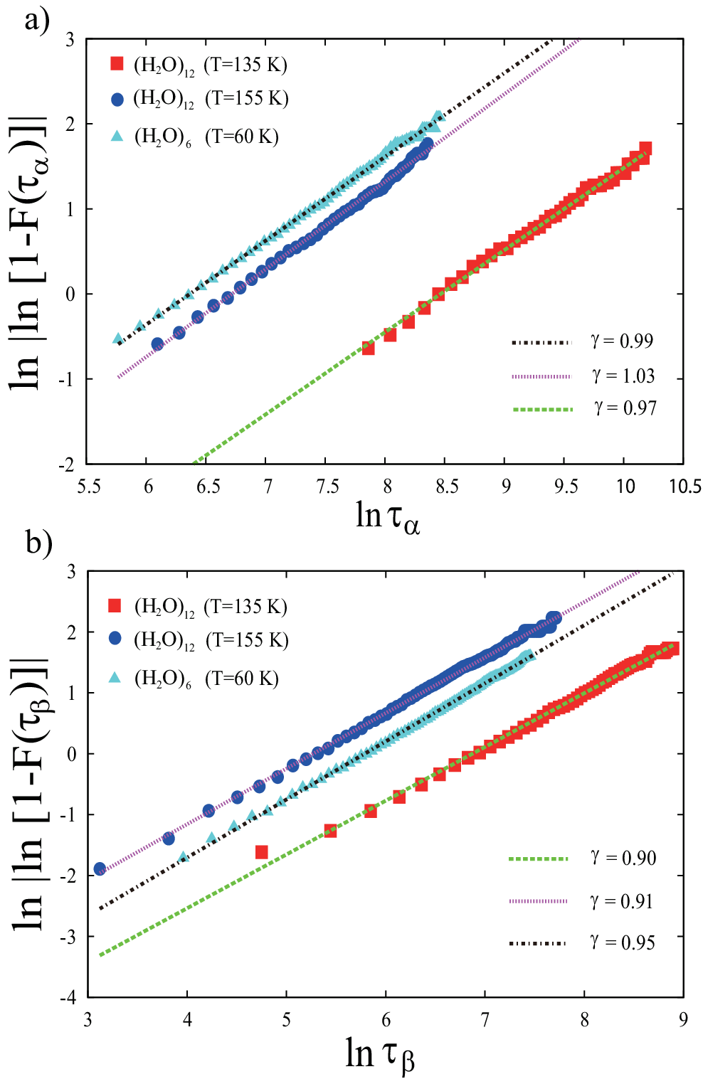
Here, we consider trapping times in the solidlike state and interevent times of large fluctuations, i.e., and . We find that the distributions of follow the Weibull distribution (see Fig. 5b):
| (9) |
where is the relaxation time for the Weibull distribution. The Weibull exponents obtained by the Weibull plot (Fig. 5) and the mean trapping time are summarized in Table 1. On the other hand, as expected in the SHN model, the distributions of follow the exponential distribution:
| (10) |
where is the relaxation time. The mean trapping time and the relaxation time are summarized in Table 1. Using the probability and the mean trapping times , we can estimate the mean and the relaxation times by [see Eqs. (6) and (8)]. The estimated values given in Table 1 are consistent with as well as the relaxation time obtained by the exponential fittings of . Therefore, the relations and are valid in water clusters.
Although the Weibull exponent of for H2O at K is almost unity, the result of the exponential distribution for is not trivial. In the disconnectivity graph for TIP4P H2O, there are two different potential minima in a solidlike state, defined by kJ/mol [21]. Because the exponential distribution cannot appear for the trapping-time distribution within many potential minima if the connectivity is sparse and inhomogeneous, the exponential distribution in originates from homogeneous connectivity between nodes within a solidlike state and those within a liquidlike state. In other words, escape probability from a metabasin (solidlike state) is always constant and does not depend on a node (potential minimum). We note that values of potential energy in the disconnectivity graph are not directly connected to our potential energy because our potential energy is averaged value.
| [K] | [ns] | [ns] | [ns] | [ns] | ||
|---|---|---|---|---|---|---|
| 135 | 0.22 | 0.90 | 1.15 | 5.25 | 5.19 | 5.39 |
| 138 | 0.22 | 0.87 | 0.96 | 4.36 | 4.12 | 4.13 |
| 142 | 0.22 | 0.88 | 0.65 | 2.95 | 2.84 | 2.89 |
| 149 | 0.22 | 0.92 | 0.37 | 1.68 | 1.50 | 1.48 |
| 155 | 0.25 | 0.91 | 0.23 | 0.92 | 0.89 | 0.84 |
IV Discussion
IV.1 Generalization of the simple homogeneous network model
We have found that transitions between solidlike and liquidlike state of water clusters are well described by the SHN model. The exponential distribution of trapping times within the solidlike state is universal in such a PEN even when the trapping-time distribution for local potential minima is not exponential. We note that trapping times in the solidlike state considered here are different from hopping times from metabasins [15], which are distributed according to a non-exponential distribution (we consider trapping times of only one specific metabasin). Non-exponential trapping-time distributions such as power laws are observed in Hamiltonian system [34], supercooled liquids, systems close to the glass transition [7, 8, 35], and biological systems [36, 37]. One of the well-known mechanisms of a non-exponential distribution is a random energy barrier model. If the heights of barriers are distributed according to the exponential distribution, the distribution of trapping times that a particle or the phase point is confined by the barriers follows a power law because of the Arrhenius law.
Here, we generalize the SHN model to provide another origin of a non-exponential distribution in a solidlike state. In the SHN model, there exists only one metabasin in the solidlike state. However, there are many metabasins in a solidlike state for large systems. On the basis of the SHN model, we consider transition dynamics between specific metabasins and the other metabasins. We assume that there are metabasins in a solidlike state and that these metabasins are not directly connected with each other (see Fig. 6). We also assume that escape dynamics from a metabasin within the solidlike state can be described by the SHN model, i.e., the exponential distribution. In particular, the trapping-time distribution in the th metabasin is described by the exponential distribution with a relaxation time . With the aid of the disconnectivity of the metabasins within the solidlike state, the trapping-time distribution within the solidlike state can be described by
| (11) |
where is the probability of a transition from the liquidlike state to the th metabasin within the solidlike state. Here we assume that the probability does not depend on a node in the liquidlike state. Therefore, the trapping-time distribution is a non-exponential distribution if the relaxation times are widely distributed. In particular, if the inverse of the relaxation times are distributed according to the Weibull distribution , the trapping-time distribution is given by a power law:
| (12) |
for . Well-known origin of a power-law trapping-time distribution are a random energy landscape and inner degrees of freedom [38]. The above scenario provides another route to a power-law trapping-time distribution, i.e., a superposition of exponential distributions, which is basically originated from the connectivities in the PEN. We note that this scenario is completely different from heterogeneous scenario in supercooled liquids [39] because the heterogeneous scenario provides a non-exponential trapping-time distribution of a particle, whereas our scenario provides that of a solidlike state.
Figure 7 shows the trapping-time distributions of and , where is set to kJ/mol, below which there are two metabasins (fused cube structure). A superposition of the exponential distributions, Eq. (11), is in good agreement with numerical simulations , indicating that two metabasins are not directly connected each other.


IV.2 Origin of the Weibull distribution in the trapping-time distribution
We have also found that interevent times of large fluctuations in the potential energy within the solidlike state are distributed according to the Weibull distribution. It has been known that there are two mechanisms generating the Weibull distribution in the trapping-time distribution. One is a random energy barrier. If the random energy barriers are distributed according to the double exponential, the trapping-time distribution obeys the Weibull distribution. For example, when the distribution of barrier heights is given by
| (13) |
the distribution of the trapping time can be described by the Arrhenius law:
| (14) | |||||
| (15) |
Therefore, the Weibull exponent depends linearly on the temperature. The mean of is given by , where .
The other mechanism of the Weibull distribution is correlated time series. If time series are strongly correlated like a spectrum, recurrence times to exceed a threshold are distributed according to the Weibull distribution [40]. If potential energy time series within the metabasin are strongly correlated, the interevent-time distribution of of large fluctuations from follows the Weibull distribution.
Arrhenius plot for the mean trapping times and is shown in Fig. 8. Arrhenius law, , seems to hold for both and , whereas the distribution of is not exponential and there are local potential minima in the solidlike state. These results are not consistent with the random energy barrier scenario because the mean interevent time does not satisfy the relation but satisfy in the random energy barrier model. Moreover, it is not clear whether the Weibull exponents given in Table I depends linearly on temperature as in Eq. (15). Therefore, the origin of the Weibull distribution is still controversial. It is interesting to clarify the origin of the Weibull distribution in small clusters. This problem is left for a future work.

V Conclusion
Introducing a concept of a solidlike state in small clusters, we have shown that dynamics regarding transitions between solidlike and liquidlike states in water clusters are well described by the SHN model proposed here, where the mean trapping time of a solidlike state is given by the mean interevent time of large fluctuations of within the solidlike state through the relation . Unlike supercooled liquids, the trapping-time distribution of a solidlike state, which is related to -process, follows the exponential distribution. Thus, processes in water clusters are completely different from those in supercooled liquids and glass transition. The exponential distribution is originated from the homogeneous connectivity between local potential minima within the metabasin and those within the other metabasins.
Appendix A Molecular dynamics simulations
The TIP4P water model [41] is used in the simulations of the water cluster. Initial coordinates are taken from the global minima of the cluster at 0 K [42], which are available from the Cambridge Cluster Database [43]. Initially, the momentum and the angular momentum are set to be zero. The MD simulations are performed in conventional canonical ensembles. The temperatures are controlled by Nosé-Hoover thermostat. The mass of thermostat per molecule is chosen to ps2 kJ/mol so that the frequency of thermostat variable becomes same as that of the vibration of oxygen to avoid the artificial dynamics by the thermostat. We confirmed that the mass of thermostat did not affect our results. The simulations were performed in free boundary condition. The integration scheme is the velocity Velret algorithm with SHAKE/RATTLE method, in which time interval is 0.5 fs. We used the MD simulation data of 250 ns for different ten initial conditions, in which the initial 0.05 ns was excluded for an equilibration.
References
- [1] M. Schmidt, R. Kusche, B. von Issendorff, and H. Haberland, Nature (London) 393, 238 (1998).
- [2] T. Kaneko, T. Akimoto, K. Yasuoka, A. Mitsutake, and X. C. Zeng, J. Chem. Theory Comput. 7, 3083 (2011).
- [3] D. J. Wales and R. S. Berry, Phys. Rev. Lett. 73, 2875 (1994).
- [4] K. Nishio and M. Mikami, J. Chem. Phys. 130, 154302 (2009).
- [5] M. Goldstein, J. Chem. Phys. 51, 3728 (1969).
- [6] F. H. Stillinger, Science 267, 1935 (1995).
- [7] P. Debenedetti and F. Stillinger, Nature (London) 410, 259 (2001).
- [8] B. Doliwa and A. Heuer, Phys. Rev. Lett. 91, 235501 (2003a).
- [9] A. Heuer, J. Phys. Condens. Matter 20, 373101 (2008).
- [10] K. Ball, R. Berry, R. Kunz, F. Li, A. Proykova, and D. Wales, Science 271, 963 (1996).
- [11] D. Wales, Energy Landscapes (Cambridge University Press, Cambridge, U. K., 2004).
- [12] T. Odagaki and Y. Hiwatari, Phys. Rev. A 41, 929 (1990).
- [13] C. Monthus and J. Bouchaud, J. Phys. A 29, 3847 (1996).
- [14] S. Büchner and A. Heuer, Phys. Rev. Lett. 84, 2168 (2000).
- [15] R. A. Denny, D. R. Reichman, and J.-P. Bouchaud, Phys. Rev. Lett. 90, 025503 (2003).
- [16] D. Watts and S. Strogatz, Nature 393, 440 (1998).
- [17] A. Barabási and R. Albert, Science 286, 509 (1999).
- [18] J. P. K. Doye, Phys. Rev. Lett. 88, 238701 (2002).
- [19] D. Wales, M. Miller, and T. Walsh, Nature 394, 758 (1998).
- [20] J. Doye, M. Miller, and D. Wales, J. Chem. Phys. 111, 8417 (1999).
- [21] D. Wales, J. Doye, M. Miller, P. Mortenson, and T. Walsh, Adv. Chem. Phys. 115, 1 (2000).
- [22] V. K. de Souza and D. J. Wales, J. Chem. Phys. 129, 164507 (2008).
- [23] V. K. de Souza and D. J. Wales, J. Chem. Phys. 130, 194508 (2009).
- [24] R. Metzler and J. Klafter, Phys. Rep. 339, 1 (2000).
- [25] W. Feller, An Introduction to Probability Theory and its Applications, 2nd ed., Vol. 2 (Wiley, New York, 1971).
- [26] K. A. Fichthorn and Y. Lin, J. Chem. Phys. 138, 164104 (2013).
- [27] K. Liu, J. Cruzan, and R. Saykally, Science 271, 929 (1996).
- [28] P. Koskinen, H. Häkkinen, B. Huber, B. von Issendorff, and M. Moseler, Phys. Rev. Lett. 98, 015701 (2007).
- [29] See Supplementary Material Document No. for movie of H2O.
- [30] See Supplementary Material Document No. for time series of potential energies in movies for H2O and H2O.
- [31] K. Koga, R. D. Parra, H. Tanaka, and X. C. Zeng, J. Chem. Phys. 113, 5037 (2000).
- [32] See Supplementary Material Document No. for movie of H2O.
- [33] S. Redner, A Guide to First Passage Time Processes (Cambridge Univ Press, Cambridge, UK, 2001).
- [34] T. Miyaguchi, Phys. Rev. E 75, 066215 (2007).
- [35] B. Doliwa and A. Heuer, Phys. Rev. E 67, 030501 (2003b).
- [36] A. V. Weigel, B. Simonb, M. M. Tamkunc, and D. Krapf, Proc. Natl. Acad. Sci. U.S.A. 108, 6438 (2011).
- [37] T. Akimoto, E. Yamamoto, K. Yasuoka, Y. Hirano, and M. Yasui, Phys. Rev. Lett. 107, 178103 (2011).
- [38] J. Bouchaud and A. Georges, Phys. Rep. 195, 127 (1990).
- [39] R. Richert, J. Phys.: Condens. Matter 14, R703 (2002).
- [40] E. G. Altmann and H. Kantz, Phys. Rev. E 71, 056106 (2005).
- [41] W. L. Jorgensen, J. Chandrasekhar, J. D. Madura, R. W. Impey, and M. L. Klein, J. Chem. Phys. 79, 926 (1983).
- [42] D. Wales and M. Hodges, Chem. Phys. Lett. 286, 65 (1998).
- [43] D. J. Wales, J. P. K. Doye, A. Dullweber, M. P. Hodges, F. Y. Naumkin, F. Calvo, and T. F. J. Hernández-Rojas Middleton, The Cambridge Cluster Database; Department of Chemistry, Cambridge University: Cambridge, U.K.; http://www-wales.ch.cam.ac.uk/CCD.html.