Compound Wishart Matrices and Noisy Covariance Matrices: Risk Underestimation
Abstract.
In this paper, we obtain a property of the expectation of the inverse of compound Wishart matrices which results from their orthogonal invariance. Using this property as well as results from random matrix theory (RMT), we derive the asymptotic effect of the noise induced by estimating the covariance matrix on computing the risk of the optimal portfolio. This in turn enables us to get an asymptotically unbiased estimator of the risk of the optimal portfolio not only for the case of independent observations but also in the case of correlated observations. This improvement provides a new approach to estimate the risk of a portfolio based on covariance matrices estimated from exponentially weighted moving averages of stock returns.
Key words and phrases:
Orthogonally invariant random matrices, Compound Wishart Matrices, Weingarten function, Markowitz problem, Risk Management1. Introduction
In practical situations in portfolio management, neither the expectation of the returns of the assets, nor the covariance matrix is known and we always deal with estimators. Since the estimators depend only on a finite number of observations, estimating the parameters of the portfolio produces a noise and as the size of the portfolio increases, the noise increases.
Here, we will focus on the noise induced by estimating the covariance matrix. Covariance matrices have a fundamental role in the theory of portfolio optimization as well as in the risk management. The concept of financial risk attempts to quantify the uncertainty of the outcome of an investment and hence the magnitude of possible losses.
In finance, the optimal portfolio is defined as that portfolio which provides the minimum risk for a certain level of return. A portfolio’s risk is the possibility that an investment portfolio may not achieve its objectives. Markowitz defined the risk of the optimal portfolio as the standard deviation of the return on the portfolio of assets. So, to determine the weights and the risk of the optimal portfolio, we essentially need to estimate the covariance matrix of the returns. To estimate the covariance matrix for a set of different assets, we need to determine entries from time series of length .
Throughout the paper, denotes the number of the assets of the portfolio and denotes the number of observations. If is not very large compared to , which is the common situation in the real life, one should expect that the determination of the covariances is noisy. In [LCBP], Laloux et al. show that the empirical correlation matrices deduced from financial return series contain a high amount of noise. Except for a few large eigenvalues and the corresponding eigenvectors, the structure of the empirical correlation matrices can be regarded as random. Unfortunately, this implies large error in estimating the risk of the optimal portfolio. Hence, Laloux et al. [LCBP] conclude that “Markowitz’s portfolio optimization scheme based on a purely historical determination of the covariance matrix is inadequate”. Improving the estimation of the risk of the optimal portfolio was an essential aim for many scientists (see [LCBP], [PGRAGS], [PK], [K]).
In ([LCBP], [PGRAGS]), it is found that the risk level of an optimized portfolio could be improved if prior to optimization, one gets rid of the lower part of the eigenvalue spectrum of the covariance matrix which coincides with the eigenvalue spectrum of the “noisy” random matrix.
For the model of normal returns, Pafka et al. [PK] and El Karoui [K], were able to compute the asymptotic effect of the noise induced from using the maximum likelihood estimator (MLE) of the covariance matrix on estimating the risk of the optimal portfolio as the ratio .
In our work, we deal with a more general estimator of the covariance matrix that encompasses and generalizes the MLE covariance. Our aim is to measure the effect of the noise induced by estimating the covariance matrix not only for the independent observations but also for the correlated observations. We essentially rely on the techniques of random matrix theory (RMT) to quantify the asymptotic effect of the noise resulting from estimating the covariance matrix on predicting the risk of the optimal portfolio. Using this asymptotic result, simulations show that we are able to provide an unbiased estimator of the risk of the optimal portfolio. In the case of independent observations, our result agrees with that of Pafka et al. [PK].
The paper is divided into four parts. In Section 2, we explain the optimal portfolio problem and give the notation used throughout the paper. We also represent some tools and techniques of random matrix theory which will be essential to prove our results. Section 3 contains our main results with proofs. In Section 4, we give some applications and simulations of our result. As an applications, we obtain the impact of the noise induced by estimating the covariance matrix for the exponentially weighted moving average (EWMA) covariance matrix. In Section 5, there will be simulations relying on real data.
2. Preliminary
2.1. Modern Portfolio Theory (MPT)
MPT is a theory in finance which attempts to maximize the portfolio expected return for a given amount of portfolio risk, or alternatively to minimize risk for a given level of expected return, by choosing the relevant weights of various assets. MPT is also considered as a mathematical form of the concept of investment diversification with the purpose of selecting a portfolio of investment assets that has collectively a lower risk than any individual asset.
MPT models an asset’s return as a normally distributed random variable, defines the risk as the standard deviation of return and models a portfolio as a weighted combination of assets so that the return of a portfolio is the weighted combination of the assets’ returns. For a portfolio of assets, the portfolio’s expected return is defined as:
where is the amount of capital invested in the asset , and are the mean returns of the individual assets.
Markowitz quantified the concept of risk using the well-known statistical measures of variance and covariance as shown in [Mark]. So, the risk on the portfolio can be associated to the total variance
where is the covariance matrix of the returns.
The goal of portfolio optimization is to find a combination of assets that minimizes the risk of the portfolio for any given level of expected return or, in other words, a combination of assets that maximizes the expected return of the portfolio for any given level of risk. One way to formulate this optimization problem mathematically is the following quadratic program:
| (1) |
where is the transpose of the dimensional vector of the optimal weights, is the dimensional vector whose th entry is , denotes the required expected reward and is the dimensional vector with in each entry.
In practice, and are unknown and we deal with estimators denoted by and , respectively. Since, in our study, we focus on the noise induced by estimating the covariance matrix and its effect on measuring the risk. We will consider the following simplified version of the portfolio optimization problem in which we deal with risky assets; i.e. none of the assets has zero variance and the covariance matrix is non-singular:
| (2) |
Using the method of Lagrange multipliers, the weights of the optimal portfolio are given by:
| (3) |
where, is the inverse of the covariance matrix .
Using (3), the risk can be expressed in terms of the entries of as follows:
| (4) |
2.2. Definition of the Problem
Since we deal with an estimator of the covariance matrix instead of itself, then for a portfolio with assets and time series of financial observations of the returns of length , we can define two kinds of risks; one using that we call the True risk, where
| (5) |
with denoting the vector of the optimal weights determined by using the entries of . The other kind of risk depends on and is called the Predicted risk, where
| (6) |
with denoting the vector of the optimal weights determined by using the entries of .
Remark 2.1.
Note that, in practice, only the Predicted risk can be computed while the True risk is unknown.
Let
| (7) |
Our goal is to have the ratio in (7) as close as possible to one. By (4), we can write
| (8) |
Clearly, this ratio is close to one as the sample size tends to infinity while remains fixed. Using results from random matrices, we are going to consider cases where and tend to infinity and . We aim to derive a deterministic bias factor which can be used to correct the above predicted risk.
2.3. Notation
For an matrix , we denote by the trace of the matrix and by the normalized trace of the matrix i.e.,
For a positive integer , . Let be the symmetric group acting on the set . For , we attach an undirected graph with vertices and edge set consisting of
Example 2.1.
Let . Then the associated graph is illustrated as shown in Figure .
Note that we distinguish every edge from even if these pairs coincide. Then each vertex of the graph lies on exactly two edges, and the number of vertices in each connected component is even. If the numbers of vertices are in the connected components of the graph, then we will refer to the sequence as the coset-type of , see [Mac, VII.2] for details. Denote by the length of the coset-type of , or equivalently the number of the connected components of .
Let be the set of all pair partitions of the set . A pair partition can be uniquely expressed in the form
with and . Then can be regarded as a permutation
We thus embed into . In particular, the coset-type and the value of for are defined.
For a permutation and a -tuple of positive integers, we define
In particular, if , then , where the product runs over all pairs in . For a square matrix and with coset-type , we define
Example (continued). For defined as in Example 2.1, the coset-type of is . This implies that and for a square matrix .
In the remaining part of this section, we present some important tools and results from random matrix theory which will play a fundamental role in our work.
2.4. Orthogonal Weingarten function
For the convenience of the reader, we supply a quick review of orthogonal Weingarten calculus. For more details, we refer to [CS, CM, Mat].
Let be the hyperoctahedral group of order . It is the subgroup of generated by transpositions and by double transpositions .
Let be the algebra of complex-valued functions on with the convolution. Let be the subspace of all -biinvariant functions in i.e.,
We introduce another product on which will be convenient in the present context. For , we define
We note that is a commutative algebra under the product with the identity element
Consider the function with a complex parameter defined by
which belongs to . For , the orthogonal Weingarten function is the unique element in satisfying
Let be the real orthogonal group of degree , equipped with its Haar probability measure. In [CM], Collins and Matsumoto formulated the local moments of the Haar orthogonal random matrices in terms of the orthogonal Weingarten functions as shown in the following proposition.
Proposition 2.1.
[CM] Let be an Haar-distributed orthogonal matrix. For two sequences and , we have
| (9) |
2.5. Compound Wishart matrices and their inverses
Compound Wishart matrices were introduced by Speicher [Sp]. They can be considered as an extension of the Wishart matrices. More precisely, they are weighted sums of independent Wishart matrices.
Let be a matrix of i.i.d. entries which are normally distributed with zero mean and unit variance i.e.,
| (11) |
Definition 2.1.
(Real Compound Wishart matrices) Let be an positive definite matrix and be a real matrix. We say that a random matrix is a real compound Wishart matrix with shape parameter and scale parameter , if
where is the symmetric root of . We write .
As shown in [BJJNPZ], if is positive-definite, then can be interpreted as a sample covariance matrix. In the sequel, we will consider to be positive definite. More details about the compound Wishart matrices can be found in [H]. For a compound Wishart matrix , if we will call a white compound Wishart matrix.
Definition 2.2.
(orthogonal invariance) Let be an real random matrix. is called orthogonally invariant if for each orthogonal matrix , has the same distribution as . We write .
Note that white compound Wishart matrices are example of such orthogonal invariant matrices.
For a portfolio with assets and time series of financial observations of the returns of length , we define a general estimator of the covariance matrix as follows:
| (12) |
where is a matrix whose rows are dimensional vectors of centered returns which are taken sequentially in time: . We assume these vectors are i.i.d. with distribution so that is the return of the -th asset at time , hence where denotes the Kronecker product of matrices and is a known weighting matrix.
Remark 2.2.
If , the identity matrix, then is the maximum likelihood estimator (MLE) of the covariance matrix which is distributed as a real Wishart matrix with degrees of freedom. The real Wishart matrices were introduced by Wishart [W] and as evidenced by the vast literature, the Wishart law is of primary importance to statistics, see ([A], [Mu]).
Since
| (13) |
Then
| (14) |
From (14), is a compound Wishart matrix with scale parameter and shape parameter . In [CMS], Collins et al. formulated the local moments of the inverted compound Wishart matrices as shown in the following theorem:
Theorem 2.1.
[CMS] Let be an compound Wishart matrix for some real matrix . Let be the inverse matrix of . Put and suppose and . For any sequence , we have
where is the pseudo inverse of the matrix .
3. Main Results
In order to derive a deterministic bias factor which can be used to improve the predicted risk of the optimal portfolio, we need to derive the following property of the inverted compound Wishart matrices. For this purpose, we show that for a compound Wishart matrix with a scale parameter and a shape parameter , the ratio between the expected trace of and the expected sum of its entries equals to the ratio between the trace of and the sum of its entries.
Proposition 3.1.
For an matrix ,
Before we prove this proposition we need to recall the following well-known fact:
Lemma 3.1.
If is an orthogonally invariant matrix, then
, where is some scalar.
is orthogonally invariant for each integer .
Proof of Proposition 3.1.
Consider
| (15) |
It is clear that is orthogonally invariant. By Lemma 3.1(ii) taking , is orthogonally invariant as well and
| (16) |
for some scalar . Another important remark is that,
| (17) | |||||
Since then, and so,
Since is invariant under cyclic permutations,
It follows that
∎
Remark 3.1.
Note that the matrix depends essentially on the dimension . So, from now on we will replace by .
In the following theorem, we study the asymptotic behavior of the ratio , defined in (7), which will play a great role in improving the prediction of the risk of the optimal portfolio.
Theorem 3.1.
Let be a real matrix such that
| (18) |
Let be as defined in (12). If , then as and tend to infinity such that , we have
| (19) |
Remark 3.2.
The condition is related to Theorem 2.1 in order to compute the second moment of the inverse of a compound Wishart matrix and to obtain a formula for the variance of the difference .
In order to prove Theorem 3.1, we need first to consider the following result concerning the variance of the ratio .
Proposition 3.2.
Proof of Proposition 3.2.
Substitute from (12) to get
| (20) |
where is an compound Wishart matrix with scale parameter and shape parameter . By applying Theorem 2.1, we get
where . By using the values of in [CM], we get
| (21) |
By applying Theorem 2.1 again, then for we get
| (22) |
where and .
From direct computations using (10) and the values of in [CM], we obtain the following equations:
| (23) |
| (24) |
and,
| (25) |
Substitute from (23), (24), and (25) into (22) to obtain
| (26) |
where and
and
By substituting from (21) and (26) into (20), the proof is complete. ∎
If , then in (12) is the MLE of the covariance matrix . For this case, Proposition 3.2 reduces to the following interesting corollary.
Corollary 3.1.
Let be as defined in (12). If , then for
| (27) |
Remark 3.3.
Note that if , then Corollary 3.1 implies that as such that , .
Now, we are ready to prove Theorem 3.1.
Proof of Theorem 3.1.
Let
The proof is divided into two parts. First, we show that
then we will prove that for
For the first part, apply Proposition 3.1 to (8) to get:
| (28) |
From (12), we have
Since is orthogonally invariant then by Lemma 3.1, we obtain
where which prove that .
This concludes the first part of the proof.
To complete the proof of the theorem, it is enough to show that for and as such that , .
Suppose that
| (29) |
By Jensen’s inequality,
| (30) |
| (31) |
Since then using Proposition 3.2 and for , can be written in terms of and as follows:
| (32) |
where
and,
Let then, from (32) and for ,
| (33) |
where
and
∎
Remark 3.4.
Remark 3.5.
Remark 3.6.
For the case , we need to compute the moments of the inverted Wishart matrices in this case which is beyond the scope of this paper.
Remark 3.7.
By Theorem 3.1, to know the asymptotic value of we need to study the asymptotic behavior of the term . As shown in [Mard] (page ), the matrix is a weighted sum of independent Wishart matrices and the weights are the eigenvalues of the matrix . So, the distribution of the matrix depends essentially on the eigenvalues of . By applying Theorem 2.1 to Theorem 3.1, we obtain the following corollary
Corollary 3.2.
Let be a real matrix and let be as defined in (12). If , and then, as and tend to infinity such that we have
| (34) |
4. Applications
In the following, we consider the case of independent observations.
4.1. The case where is an idempotent
Let be an idempotent matrix i.e., . If has rank then, has nonzero eigenvalues and each eigenvalue equals one. In this case, condition (18) holds and is a white Wishart matrix with degrees of freedom. From Corollary 3.2, as and tend to infinity and ,
| (35) |
4.1.1. Example: Maximum Likelihood Estimator (MLE)
is a maximum likelihood estimator of if in (12). For this estimator, is an idempotent of rank . From (35), we get the following result.
Corollary 4.1.
If is the MLE of , then as and tend to infinity such that , we have
This result coincides with the result of Pafka and Kondor in [PK].

To simulate this case, we randomly choose a value for . Using this value, we compute the True risk. Second, we generate a set of observations from the distribution and estimate and using these observations. Finally, we compute the Predicted risk using the MLE covariance and compare the Predicted and the True risks. As shown in Figure (), we get a remarkable improvement in estimating the risk for MLE after scaling the Predicted risk using the factor in Corollary 4.1. The figure illustrates the ratio between the Predicted and the True risks before and after applying Corollary 4.1. The dotted line in each histogram represents the mean of the ratio between the two risks. For the middle graphs of the figure, we take and and for these values the mean of the ratio between the risks before and after scaling equals and , respectively which shows a remarkable improvement in computing the Predicted risk.
To study the validity of the Scaling technique for small values of , we take and and as shown in the upper graphs of Figure ,
the mean of the ratio between the risks before and after scaling is and , respectively. So, the Scaling technique is still valid for small dimensions and small observations situations.
In the lower graphs of Figure , we choose closed values for and ( and ) and the mean of the ratio between the risks equals
and before and after scaling, respectively. From the simulations, we conclude that for the MLE, the Scaling technique is a real
improvement in estimating the risk. Also, note that the reduction in the standard deviation of the ratio of the Predicted and the True risks from the upper graph to the middle graph as and increases from and to and . In theory, the standard deviation goes to zero an and tend to infinity such that by Corollary 4.1.
4.2. When the Expected Returns are unknown
The unbiased estimator of the covariance matrix is called the sample covariance matrix and is given by
The sample covariance estimator can be obtained from (12) by considering the entries of the matrix as follows:
In this case, is an idempotent of rank . In [K], El-Karoui shows that the asymptotic behavior of the noise resulting from estimating the covariance matrix using the sample covariance estimator (with unknown expected means of the returns) is which still coincides with our result in (35) although in our case we assume the returns are centered. This similarity between the two cases is due to the independence between the estimators and . To simulate this case, we randomly choose values for and . Using these values, we compute the True risk. Next, we generate a set of observations from the distribution and estimate and using these observations. Finally, we compute the Predicted risk using the estimators and and compare the Predicted and the True risks. As shown in Figure (), the ratio between the scaled Predicted risk and the True risk is very close to one and there is a valuable improvement in estimating the Predicted risk after using the Scaling technique.
In the next section, we are going to study an important estimator of the covariance matrix which plays a great role in many fields, specially in finance

4.3. Exponentially Weighted Moving Average (EWMA)
In the stock market, using equally weighted data doesn’t accurately exhibit the current state of the market. It reflects market conditions which are perhaps no longer
valid by assigning equal weights to the most recent and the most distant observations. To express the dynamic structure of the market, it is better to
use exponentially weighted variances. Exponentially weighted data gives greater weight to the most recent observation. Thus, current market conditions are taken into consideration more accurately. The EWMA model is proposed by Bollerslev [Bol]. Related studies ([F], [T]) are made in the equity market and using exponentially weighted moving average techniques (weighting recent observations more heavily than older observations). In [Ak], Akgiray shows that using EWMA techniques are more powerful than the equally weighted scheme.
In EWMA technique,
returns of recent observations to distant ones are weighted by multiplying each term starting from the most recent observation by an exponential decay
factor ) respectively. In common, is called the decay factor.
Hence, in (12), for and we have
If , then . Now, let us apply Theorem 3.1 to the EWMA estimator and obtain the following corollary.
Corollary 4.2.
Let be the EWMA estimator of the covariance matrix with decay factor . If then, as tend to and as tend to infinity such that (for some positive constant ) and , we have

As shown in Figure , for the EWMA covariance matrices, scaling the Predicted risk using Corollary 4.2 gives a great improvement to estimate the risk of the optimal portfolio. Before scaling as illustrated in the graphs on the left hand side of Figure , the ratio between the two risks is far from specially for close values of and () as shown in the lower left graph of the figure. After scaling the Predicted risk by the factor as in Corollary 4.2, the ratio between the Predicted and the True risks becomes very close to as in the right hand sides graphs of the figure. For small values of and , as in the upper graphs of the figure, and , the means of the histograms of the upper graphs, represented by the dotted line in each histogram, equal (before scaling) and (after scaling). So, the Scaling technique still works and improves the estimation of the Predicted risk. Again note the reduction in the standard deviation of the ratio of the Predicted and the True risks from the upper graph to the middle graph as and increases from and to and .
5. Real Data
In this section, we work with real data from the stock market and observe the effect of using the scaling technique on improving the prediction of the risk of the optimal portfolio. For stocks, , we compute the True risk using a large number () of observations. In order to compute the Predicted risk, we use only observations i.e., .
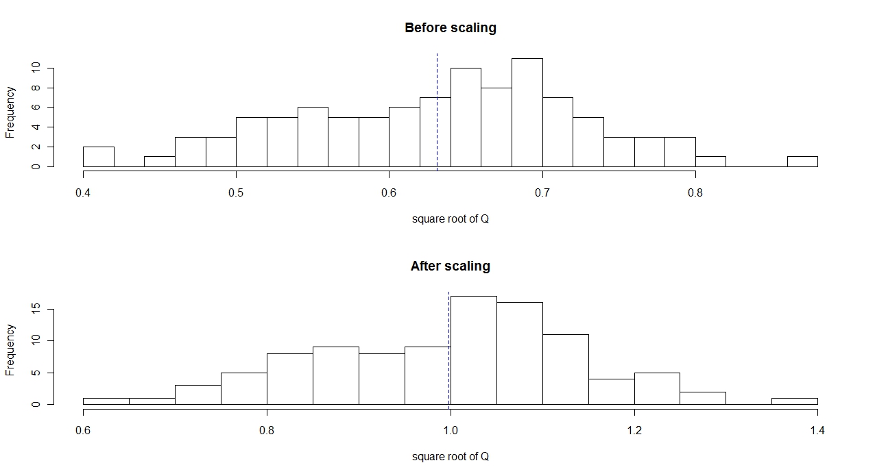
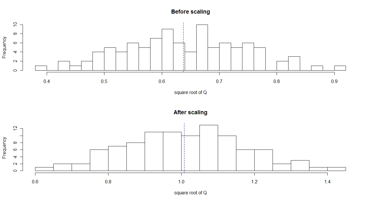
To compute the Predicted risk, we randomly choose observations and use them to find the MLE (or EWMA) of the covariance matrix and then invert the MLE (or EWMA) and calculate the Predicted risk. After repeating this process for times, we histogram the ratio between the Predicted and the True risks before and after scaling using the result of Corollary 4.1 (or Corollary 4.2 in the case of EWMA covariance).
In Figure , we illustrate the ratio between the Predicted and the True risks in the case of the MLE covariance. As shown in the upper histogram, the average of the ratio between the risks is before scaling. While after scaling, the average of the ratio between the risks is as shown in the lower histogram. This shows that using Corollary 4.1, in the case of MLE covariance, admits a real improvement in estimating the risk of the optimal portfolio.
In the case of the EWMA covariance, we choose some value for the decay factor e.g. and illustrate the ratio between the Predicted and the True risks before and after scaling using Corollary 4.2 as shown in Figure . In the upper histogram, the average of the ratio between the risks is before scaling. While after scaling, as shown in the lower histogram, the ratio between the risks becomes . Hence, for the EWMA covariances, using the result of Corollary 4.2 provides a better estimation of the risk of the optimal portfolio. We conclude that the scaling technique admits a good prediction of the risk of the optimal portfolio for different covariance matrices.
Remark 5.1.
In the case of EWMA, we take different values for the decay factor and in each time the ratio between the Predicted and the True risks becomes closer to one after using the Scaling technique.
6. Conclusion
For a general estimator of the covariance matrix and using our results concerning the moments of the inverse of the compound Wishart matrices, we are able to use a Scaling Technique to cancel the asymptotic effect of the noise induced by estimating the covariance matrix of the returns on the risk of an optimal portfolio. As an application, we get a new approach on estimating the risk based on estimating the covariance matrices of stocks returns using the exponentially weighted moving average. Simulations show a remarkable improvement in estimating the risk of the optimal portfolio using the Scaling technique which outperforms the improvement obtained by using the Filtering technique [BiBouP].
We believe that the effect of noise on computing the risk and the weights of the optimal portfolio results from estimating the inverse of the covariance matrix (using the inverse of the estimator of the covariance matrix) not from estimating the covariance matrix itself. Improving the estimator of the inverse of the covariance matrix is an interesting topic for our future work.
Acknowledgments
B.C, D.McD. and N.S. were supported by NSERC discovery grants B.C. and N.S. were supported by an Ontario’s ERA grant. B.C. was supported in part by funding from the AIMR.
The authors would like to thank M. Alvo, M. Davison, R. Kulik and S. Matsumoto for support and enlightening discussions.
References
- [Ak] V. Akgiray, Conditional Heteroscedasticity in Time Series of Stock Returns: Evidence and Forecasts, Journal of Business 62: 55-80, 1989
- [A] T. W. Anderson, An introduction to multivariate statistical analysis, third ed. Wiley Series in Probability and Statistics. Wiley-Interscience [John Wiley & Sons], Hoboken, NJ, 2003.
- [B] P. Billingsley, Probability and Measure, 3rd edn, J. Wiley & Sons, Inc., 1995.
- [BiBouP] G. Biroli, J.-P. Bouchaud, M. Potters, 2007. The Student Ensemble of Correlation Matrices, Acta Phys. Pol., B 38.
- [Bol] T. Bollerslev, Generalised Autoregressive Conditional Heteroscedasticity, Journal of Econometrics 31: 307-327, 1986.
- [BP] J. P. Bouchaud and M. Potters, Theory of Financial Risk, Cambridge University Press, 2000.
- [BJJNPZ] Z. Burda, A. Jarosz, J. Jurkieewicz, M. A. Nowak, G. Papp and I. Zahed, Applying free random variables to random matrix analysis of financial data. arXiv.org:physics/0603024, 2006.
- [CM] B.Collins and S. Matsumoto, On some properties of orthogonal Weingarten functions, J. Math. Phys.50, 113516, 2009.
- [CMS] B. Collins, S. Matsumoto and N. Saad, Integration of invariant matrices and application to Statistics,, arxiv.org/abs/1205.0956, 2012.
- [CS] B. Collins and P. Śniady, Integration with respect to the Haar measure on unitary, orthogonal and symplectic group, Comm. Math. Phys. 264(3): pp. 773-795, 2007.
- [K] N. El Karoui, High Dimensionality Effects in The Markowitz Problem and Other Quadratic Programs with Linear Equality Constraints: Risk Underestimation, The Annals of Statistics, 2009.
- [[EG] E. J. Elton and M. J. Gruber, Modern Portfolio Theory and Investment Analysis J.Wiley and Sons, New York, 1999; H. Markowitz, Portfolio Selection: Efficient Diversification of Investments, J.Wiley and Sons, New York, 1959.
- [F] E. Fama, The Behaviour of Stock Market Prices, Journal of Business, 38: pp. 34-105, 1965.
- [H] F. Hiai and D. Petz, The semicircle law, free random variables and entropy, vol. 77 of Mathematical Surveys and Monographs. American Mathematical Society, Providence, RI, 2000.
- [LCBP] L. Laloux, P. Cizeau, J.-P. Bouchaud and M. Potters, Random matrix theory and financial correlations. International Journal of Theoretical and Applied Finance, 3: pp. 391-397, 2000.
- [Mac] I. G. Macdonald, Symmetric Functions nad Hall Polynomials, 2nd ed.. Oxford University Press, Oxford, 1995.
- [Mard] K. V. Mardia, J. T. Kent and J. M. Bibby, Multivariate analysis. Academic Press [Harcourt Brace Jovanovich Publishers], London. Probability and Mathematical Statistics: A Series of Monographs and Textbooks, 1979.
- [Mark] H. Markowitz, Portfolio Selection, The Journal of Finance 7 (1): pp. 7791, 1952.
- [Mat] S. Matsumoto, General moments of the inverse real Wishart distribution and orthogonal Weingarten functions, arXiv:1004.4717v3, 2011.
- [Mu] R. J. Muirhead, Aspects of multivariate statistical theory, John Wiley & Sons Inc., New York, 1982.
- [PK] S. Pafka and I. Kondor, Noisy covariance matrices and portfolio optimization II, Phys. A 319: pp. 487-494, 2003.
- [PGRAGS] V. Plerou, P. Gopikrishnan, B. Rosenow, L. A. N. Amaral, T. Guhr and H. E. Stanley, e-print cond-mat/0108023; B. Rosenow, V. Plerou, P. Gopikrishnan and H. E. Stanley, e-print cond-mat/0111537.
- [Sp] R. Speicher, Combinatorial theory of the free product with amalgamation and operator-valued free probability theory, Mem. Amer. Math. Soc., 132, 1998.
- [T] Y. Tse, Stock Return Volatility in the Tokyo Stock Exchange, Japan and the World Economy, 3: pp. 285-298, 1991.
- [W] J. Wishart, The generalised product moment distribution in samples from a normal multivariate population, Biometrika, 20A: pp. 32-52, 1928.
Benoît Collins
Département de Mathématique et Statistique, Université d’Ottawa,
585 King Edward, Ottawa, ON, K1N6N5 Canada,
WPI AIMR, Tohoku, Sendai, 980-8577 Japan
and
CNRS, Institut Camille Jordan Université Lyon 1,
France
bcollins@uottawa.ca
David McDonald
Department of Mathematics and Statistics, University of Ottawa,
585 King Edward, Ottawa, ON, K1N6N5 Canada
Nadia Saad
Department of Mathematics and Statistics, University of Ottawa,
585 King Edward, Ottawa, ON, K1N6N5 Canada
nkotb087@uottawa.ca