The macroscopic monopolization in diagonal magnetoelectrics
Abstract
We develop the formalism of the macroscopic monopolization – that is the monopole moment per unit volume – in periodic solids, and discuss its relationship to the diagonal magnetoelectric effect. For the series of lithium transition metal phosphate compounds we use first-principles density functional theory to calculate the contributions to the macroscopic monopolization from the global distribution of magnetic moments within the unit cell, as well as from the distribution of magnetization around the atomic sites. We find one example within the series (LiMnPO4) that shows a macroscopic monopolization corresponding to a ferromonopolar ordering consistent with its diagonal magnetoelectric response. The other members of the series (LiMPO4, with M = Co, Fe and Ni) have zero net monopolization but have antiferromonopolar orderings that should lead to -dependent diagonal magnetoelectric effects.
I Introduction
The linear magnetoelectric response of a solid is the linear order magnetization induced by an electric field or equivalently the linear order electric polarization induced by a magnetic field. It is described by a second-rank tensor, , which can be non-zero when both time-reversal and space-inversion symmetries are broken, and may have diagonal or off-diagonal components, corresponding to a response parallel or perpendicular to the applied field respectively.
Materials with anti-symmetric off-diagonal linear magnetoelectric responses have the same symmetry as the toroidal component of the second-order term in the magnetic multipole expansion, and so there has been much recent discussion in the literature of whether the toroidal moment, , is a relevant and useful concept for describing such magnetoelectric effects. In particular, the term ferrotoroidics has been introduced to describe materials in which the toroidal moments are aligned cooperatively, and such materials have been considered to complete the group of primary ferroics.[1, 2, 3] Motivated by this suggestion, a theory of toroidization – defined to be the toroidal moment per unit volume – in bulk crystalline solids has been developed, which appropriately treats the multi-valuedness caused by the periodic boundary conditions [4]. Ferrotoroidic switching has been reported [3], and attempts to demonstrate that the toroidal moment can act as a primary order parameter are ongoing. In addition, the local toroidal moments associated with the atomic V sites in V2O3 and the atomic Cu sites in CuO have been detected directly using resonant x-ray diffraction [5, 6, 7]. Such local toroidal moments could be of tremendous importance, as it has been proposed that they are candidates for the order parameter in the pseudo-gap phase of cuprate superconductors[8].
The second-order term in the magnetic multipole expansion contains two additional contributions beyond the toroidal term, which describe in turn magnetic quadrupolar and magnetic monopolar components that couple respectively to the gradient and divergence of the magnetic field (see detailed derivation below). While the latter has not been extensively discussed on the grounds that Maxwell’s equations tell us formally that does not diverge, it is in fact non-zero in materials with a diagonal linear magnetoelectric response. Indeed, it could appropriately be described as a magnetoelectric monopole to distinguish it from the zeroth order term in the multipole expansion of the magnetic field which is the magnetic analogue to the electrical charge and indeed is formally zero. We emphasize also that the magnetoelectric monopole discussed here is a ground state property of the system, and so is distinct from those recently proposed and verified in spin ice, in which nonlocal magnetic monopoles exist as excited states [9, 10].
The origin of the relationship between the monopolar contribution to the multipole expansion and the diagonal magnetoelectric response is illustrated in Fig. 1 (a) and (b) where we follow the discussion from Ref. 11. The monopolar magnetic vortex in panel (a) consists of local spin magnetic moments (black solid arrows) oriented outwards from a point – note that Maxwell’s equations are not violated; while diverges, it is compensated for by and so does not diverge. Since the spin moments are never parallel, it is known from the theory of multiferroics that there is a local radial electric polarization (unfilled grey arrows) associated with each pair of spins [12, 13]. However these local radial polarizations are uniform around the vortex and the net electric polarization is zero. On application of a magnetic field, however, the spin moments reorient to align themselves more closely parallel to the field (panel (b)). The local contributions to the electric polarization no longer average to zero and a net polarization parallel to the magnetic field direction results.
For completeness, we show in Figure 1 (c) and (d) the analogous relationship between a toroidal vortex and the off-diagonal magnetoelectric response. In this case an applied magnetic field modifies the spin orientations so that a net magnetic moment is induced perpendicular to the direction of applied field.

The remainder of this paper is organized as follows: In the next section we review the definition of the magnetoelectric monopole starting from a multipole expansion of the magnetic field and show that it couples to the divergence thereof. In Section III we describe how the monopole can be calculated from first-principles electronic structure methods, as well as how it could be directly measured experimentally. We introduce the term monopolization to describe the monopole per unit volume in periodic solids, and show that it is natural both theoretically and experimentally to divide the total monopolization into two contributions: That arising from the local monopoles around individual ions, and that arising from the global distribution of magnetic moments within the solid. We discuss also the problems associated with defining the monopolization for an infinite periodic solid, and propose a practical solution. In Section IV we present results of the calculated monopolizations for the family of lithium transition metal phosphates, LiMPO4, M = Mn, Fe, Co, Ni. All members of this family have the same structure and overall magnetic order, but they differ in their local magnetic anisotropy and hence their magnetic symmetry. We find that the different magnetic symmetries lead to different monopolar orderings: In one case there is ferromonopolar ordering with a net macroscopic monopolization, and the remaining three cases have zero net monopolization, but with hidden “anti-ferromonopolar” orderings that have not previously been identified. In section V we develop the Ginzburg-Landau theory describing the coupling of the monopolization to homogeneous external magnetic and electric fields. In the final section we discuss the possible relevance of these concepts.
II The multipole expansion
Following the derivation in Ref. 14, we consider a magnetization density , that may arise from both spin and orbital contributions, in an inhomogeneous magnetic field that varies slowly on the scale of the system size. Then the interaction energy, , of the magnetization density with the magnetic field
| (1) |
can be expanded in powers of field gradients calculated at some arbitrary reference point :
| (2) |
where are Cartesian directions. The first term is the interaction of the field with the magnetic moment of the system
| (3) |
In the second term, the tensor with nine components can be decomposed into three parts (summation over repeated indices is implied):
- i)
the pseudoscalar from the trace of the tensor,
(4)
- ii)
the toroidal moment vector dual to the antisymmetric part of the tensor, ,
(5) and
- iii)
the traceless symmetric tensor describing the quadrupole magnetic moment of the system,
(6)
The expansion of Eqn. (2) can then be written in the form
| (7) | |||||
We see that the toroidal moment couples to the curl of the magnetic field, and the quadrupole moment couples to the field gradient, while the pseudoscalar is coupled to the divergence of magnetic field, and so represents a monopolar component.
III Calculation and measurement of the magnetoelectric monopole in bulk, periodic solids
In this section we discuss the difficulties associated with the definition of the monopole in bulk, periodic solids, and propose solutions that allow a correspondence between calculated monopole moments and possible experimental measurements. First we note a simplification: Since the orbital contribution to the magnetization density, is proportional to , where is the momentum, and is zero, the orbital contribution to the monopole is always formally zero, and only the spin contribution need be considered.
For systems of finite size, such as molecules or molecular clusters, that have zero net magnetic moment, the value of the monopole can be evaluated directly from the spin part of the magnetization density through the integral in Eqn. 4. Eqn. 4 is not directly applicable to extended systems where periodic boundary conditions are employed, however, because the integral contains the position operator, . Therefore for a general continuous magnetization density it will lead to arbitrary values, depending on the choice of unit cell used in the calculation.
III.1 Decomposition of the monopole moment into atomic site and local moment contributions
In anticipation of treating the bulk, periodic case, we re-write Eqn. 4 by decomposing the position operator into the positions of the constituent atoms, , relative to some arbitrary origin, plus the distance from each atomic center, . The integral over all space then separates into a sum over the atomic sites, and an integral around each atomic site, , and Eqn. 4 can be rewritten as
| (8) | |||||
where the summation, is over all of the atoms in the system, and is the local magnetic moment on the th atom.
We see then that the monopole can be decomposed into two components: The first, comes from the local monopoles at the atomic sites, which arise from the same current distribution around the site that simultaneously gives rise to the local dipole moment. We call this contribution for “atomic site”, and at each site, , it is given by
| (9) |
where the atomic nucleus is at position and the integral is over some localized region around the atomic nucleus; in an electronic-structure calculation this can be chosen to be the “atomic sphere” or the “pseudo-atomic orbital” depending on the details of the implementation and the integral can in principle be evaluated over this finite region.
In practice, we calculate the atomic site contributions to the monopole through expectation values of spherical tensors using a generalization of the method used previously to obtain inversion-even tensor moments in studies of correlated or electron materials[15, 16]. For each atomic site a local density matrix inside a site-centered sphere is obtained from the electronic structure and expanded in spherical harmonics and spinors. In the present work we use the augmented plane wave plus local orbital (APW+lo) method and these spheres are naturally chosen to be the muffin-tin spheres. The density matrices are then further expanded with respect to their behavior (either even or odd) under space inversion and time inversion :
| (10) |
For magnetoelectrically active multipole moments such as monopoles, only the component that is odd in both space inversion and time reversal that is , is relevant. In addition, for convenience we expand the density matrices in the Pauli matrices and the identity matrix in spin space,
| (11) |
where is the trace over the spin degree of freedom.
Now the monopole moment can be written in the form
| (12) |
Here the operator describes the coupling of two rank one tensors, and , to a rank zero , and and is the trace over the orbital degree of freedom. In Figure 2 we show the generic magnetization textures for positive and negative atomic site monopoles, as well as for completeness the component of a toroidal moment and the component of the quadrupolar tensor. The arrows represent the magnetization orientation on a sphere surrounding an atomic site and the color indicates whether the magnetization points outwards (green) or inwards (red).

Note that these atomic site monopoles can in principle be measured by resonant x-ray spectroscopy[17], which has been used successfully to detect an atomic site toroidal moment[18, 7]. No unambiguous measurement of atomic monopoles has been made to date, however, because a material has not yet been identified that meets the stringent conditions required to achieve an observation in the resonant x-ray measurement. We point out also that, provided that the local magnetic site is not an inversion center, the atomic monopoles can be non-zero even in a system with overall zero monopole moment; we will explore some examples in Section IV. Such systems might be described as “anti-monopolar” and should show a -dependent magnetoelectric effect.
The second contribution to the monopole, which we write for “local moment”, arises from representing the magnetization density by a distribution of localized magnetic moments at the atomic sites:
| (13) |
In systems such as insulating transition metal oxides, which have large localized magnetic moments that are spatially separated by distances of a few Å we expect this contribution to be the dominant contribution to the total monopole.

Using Eq. (13) we can straightforwardly evaluate the monopoles of the arrangements of magnetic moments shown in Fig. 3. Taking the -oriented magnetic moments to be spaced a distance apart along the direction, and the -oriented moments a distance apart along , then the monopoles of arrangements a) and b) in Fig. 3 are and respectively, where is the magnitude of each local magnetic dipole moment. Applying Eq. 13 to the arrangement show in c) yields the value ; this can also be obtained by inspection by recognizing that c) consists of a monopole with magnetic moments at the same position of as in b) but of half the magnitude, plus a quadrupole, as shown in the lower panel of Fig. 3.
The total monopole resulting from these two contributions is then
| (14) |
where the sum is over all the atomic sites.
In all the cases shown in Fig. 3, the net magnetization is zero. There exists a complication, however, in the case where the region over which the monpole is to be evaluated has a net magnetic dipole. The complication is that all multipoles in systems with non-zero lower-order multipoles (the magnetic dipole in the case of the magnetoelectric monopole) are dependent on the choice of origin used to evaluate them. It is straightforward to see that for systems with nonvanishing magnetic dipole moment, for a change of origin defined by
| (15) |
the monopole changes as
| (16) |
It remains an open question in general, which we do not address here, whether such origin dependence of the multipoles is physically meaningful (see for example Ref. 19). One practical approach is to always choose as the origin the position of the average magnetic moment, , defined so that This is equivalent to neglecting any uncompensated part of the magnetization and retaining only the compensated part in the calculation of the monopole[4]. Care must be taken, however, in situations where a change in net magnetic dipole moment, or a structural rearrangement occurs, to ensure that a consistent choice of origin is maintained.
III.2 Bulk systems with periodic boundary conditions; the problem of multi-valuedness
Next we turn to the case of a system with periodic boundary conditions. It is often convenient to describe the properties of a bulk crystalline solid in terms of a small repeat unit – the unit cell – which is then replicated using periodic boundary conditions to generate the infinite solid. Many intensive quantities such as the magnetization, which is defined to be the magnetic moment per unit volume, can then be simply obtained as the value of the quantity in a single unit cell divided by the unit cell volume. For the case of the macroscopic monopole per unit volume – which we propose to call the monopolization by analogy with magnetization, polarization, etc. – Eqn. 4 is not directly applicable to extended systems with periodic boundary conditions, because for a general continuous magnetization density , Eq. (4) evaluated over one unit cell will lead to arbitrary values, depending on the particular choice of unit cell used in the calculation. We note that this behavior is distinct from the origin dependence discussed in Section III.1, and persists even in the case when the net magnetization is zero. In fact the difficulties are exactly analogous to those encountered in defining a macroscopic bulk toroidization, and indeed reflect those involved in defining a macroscopic bulk ferroelectric polarization, which were solved through the introduction of the modern theory of polarization[20, 21, 22]. A proposed solution in the case of the toroidization was described in detail in Ref. 4. In this section we extend the description to the case of the monopole and address the following questions:
- 1.
How should the monopole density – the monopolization – of a bulk periodic solid be formally defined?
- 2.
What are the consequences of the periodic boundary conditions within a bulk crystalline solid?
For simplicity we develop the formalism for the case of the monopolization coming from the local moment contribution. First we note that, as we shall see later, the formalism requires that each local moment, , is equal to an integer number of Bohr magnetons. Since we consider only the spin part of the magnetic moment (the orbital part does not contribute to the monopole), a magnetic moment that is an integer number of Bohr magnetons corresponds to the moment of an integer number of electrons. In general, however, an integer number is not obtained from integrating the magnetization density over a sphere around an atomic site in a solid; in fact this number is not uniquely defined as it depends on the choice of integration radius. Rather, the spin moment of the corresponding spin-polarized Wannier function should be used; since a Wannier function in an insulating system contains an integer number of electrons its spin is always an integer number of Bohr magnetons.
We then define the local moment monopolization, , where is the volume of the system with local moment monopole . Then, for a large finite system containing identical unit cells each of volume :
| (17) | ||||
| (18) |
Here, are the positions of the magnetic moments relative to the same (arbitrary) point within each unit cell, is a lattice vector with index , and we have used the fact that the orientation of the magnetic moments is the same in each unit cell. The summation over indicates the summation over all moments within a unit cell, and that over indicates the summation over all unit cells. Expanding the scalar product, we obtain:
| (19) |
using the fact that the sum over all lattice vectors contains both and , so that . Thus, the local moment monopole of a system of unit cells is just times the monopole evaluated for one unit cell, and the corresponding monopolizations are identical.
In an infinite periodic solid, we have a freedom in choosing the basis corresponding to the primitive unit cell of the crystal. In particular, we can translate any spin of the basis by a lattice vector without changing the overall periodic arrangement. However, such a translation of a spin by leads to a change in the local moment monopolization as follows:
| (20) |
where is a unit vector oriented in the direction of magnetic moment . The freedom in choosing the basis corresponding to the primitive unit cell thus leads to a multivaluedness of the monopolization with respect to certain “increments” (defined by Eq. (20)) for each magnetic sub-lattice and lattice vector .
This multivaluedness of the monopolization is reminiscent of the modern theory of electric polarization,[22, 23, 21] where the polarization changes by when an elementary charge is translated by a lattice vector . The resulting multivaluedness has led to the concept of the “polarization lattice” corresponding to a bulk periodic solid,[23] with called the “polarization quantum” if is one of the three primitive lattice vectors. An even closer analogy is provided by the toroidization, which is multivalued with values spaced by the toroidization increment , corresponding to translation of an elementary magnetic moment, by a lattice vector [4]. Eq. (20) suggests the existence of an analogous “monopolization lattice”, with monopolization increments , where is any primitive lattice vector and are the unit vectors indicating the orientations of the magnetic moments. Note that the monopolization, and hence the monopolization increments are scalar quantities. As a result the corresponding monopolization lattice can become rather dense, particularly in cases where the three lattice vectors are unequal but close in size, and the spin moments are noncollinear and canted away from the lattice vector directions.
We illustrate the behavior and implications of the monopolization lattice next with a simple model one-dimensional example.
III.3 A one-dimensional example
The periodic non-monopolar state.

To illustrate some consequences of the multivaluedness of the monopolization in periodic systems described in the previous section, we now consider the example of a one-dimensional antiferromagnetic chain of equally spaced magnetic moments as shown in Fig. 4a. The moments, with magnitude , are spaced a distance apart from each other along the axis, and are alternating in orientation along . Thus, the unit cell length is and there are two oppositely oriented magnetic moments in each unit cell. Since this configuration does not possess a macroscopic magnetic dipole moment, the corresponding monopole moment is origin independent.
The arrangement of magnetic moments in Fig. 4a is space-inversion symmetric with respect to each moment site and thus cannot exhibit a macroscopic monopole moment. The local moment monopole of the single unit cell highlighted in Fig. 4a, calculated using Eq. (13), however, is identical to that calculated for the finite moment configuration in Fig. 3c, i.e. , and the corresponding monopolization, (since the “volume” of the one-dimensional unit cell is just its length, ). Since the moments of magnitude are oriented exactly parallel to the axis, the elementary monopolization increment in this case is , which means that the monopolization of the unit cell is exactly equal to one half of the monopolization increment, and the allowed monopolization values for the periodic arrangement are , where can be any integer number.
We see that in our example the allowed local moment monopolization values form a one-dimensional lattice of values, centrosymmetric around the origin. This is analogous to the cases of the electric polarization and the toroidization, where the polarization and toroidization lattices are invariant under all symmetry transformations of the underlying crystal structure. In particular, the polarization and toroidization lattices corresponding to centrosymmetric crystal structures are inversion symmetric, which is achieved in lattices that include either the zero or the half quantum/increment. We see that the same holds true for the local moment monopolization of our one-dimensional example, and that a centrosymmetric set of monopolization values can be understood as representing a non-monopolar state of the corresponding system. We also note that the formalism is only consistent for the case of local magnetic moments corresponding to integer numbers of Bohr magnetons, which in turn correspond to the spin contribution from integer numbers of electrons.
In the case of the electric polarization, it is now widely recognized that only differences in the polarization lattices between different configurations, such as between a centrosymmetric non-polar reference structure and a ferroelectric polar crystal, are in fact measurable quantities. Since these differences are the same for each point of the polarization lattice they are well-defined quantities. Likewise in the case of the toroidization, only differences in toroidization lattices between for example different arrangements of magnetic moments or different ionic positions are measurable[4]. In the next section we show that, in analogy with the cases of the toroidization and electric polarization, only differences in local moment monopolization, corresponding to two different bulk configurations, are measurable quantities and correspond to physical observables such as the difference in monopolization between a ferromonopolar state and its non-monopolar paraphase. Such quantities can be obtained by monitoring the change in monopolization on one arbitrarily chosen branch within the allowed set of values, when transforming the system from the initial to the final state along a well-defined path.
Monopolar state and changes in monopolization.
In order to obtain a nontrivial macroscopic monopolization the system has to break both space and time inversion symmetry. In the case of the one-dimensional antiferromagnetic chain this can be achieved by “moment pairing”, i.e. if the distances between neighboring magnetic moments alternate as shown in Fig. 4b. Here the magnetic moments of magnitude are spaced alternately a distance of and apart from each other along the axis (). The non-monopolar example above corresponds to . Since the unit cell size is the same as in the non-monopolar case, the elementary monopolization increment is again . The monopolization of the unit cell indicated in Fig. 4b is , so that the allowed values of for the full periodic arrangement are:
| (21) |
Fig. 5 shows the allowed monopolization values as a function of the displacement of the moments from their positions in the centrosymmetric, non-monopolar state.

The change in monopolization between two configurations with and for a certain branch is given by:
| (22) |
i.e. it is independent of the branch index . In particular, if the non-centrosymmetric distortion is inverted (, , the change in monopolization is so that can be interpreted as the spontaneous monopolization, again in analogy to the case of the electric polarization, where the spontaneous polarization is given by the branch-independent change in polarization compared to a centrosymmetric reference structure.
Another possible way to alter the monopolization is by changing the orientation of the magnetic moments instead of changing their positions. In particular, we expect that a full 180∘ rotation of all magnetic moments, which is equivalent to the operation of time reversal, should invert the macroscopic “spontaneous monopolization”, and should therefore lead to the same change as discussed above. If we allow the magnetic moments to rotate out of the direction, while preserving the antiparallel alignment of the two basis moments, the monopolization is given by
| (23) |
where is the angle between the magnetic moments and the direction. Note here a difference from the case of the toroidization – since the monopolization is a scalar, rotation of the magnetic moments away from perfect alignment reduces the absolute magnitude of the monopolization. In contrast, in the toroidal case a rotation could reduce the toroidization along one axis while simultaneously increasing it along another. Interestingly, in this example, the magnetic moment rotation which reduces the monopolization induces a toroidization, effectively converting the monopolar response into a toroidal one through the moment reorientation. The change in monopolization for a full 180∘ rotation of the moments is thus:
| (24) |
and apparently depends on the branch index . However, if one calculates the same change in monopolization for the non-monopolar state with , one obtains:
| (25) |
Obviously, in this case the corresponding change in macroscopic monopolization should be zero, since both the initial and final states (and all intermediate states) correspond to a non-monopolar configuration and thus . If one subtracts the improper change in , Eq. (25), from the change in monopolization calculated in Eq. (24), one obtains the proper change in monopolization , which is identical to that obtained by inverting the non-centrosymmetric distortion . Here, we use the terminology “proper” and “improper” in analogy to the case of the proper and improper piezoelectric response, [24] where a similar branch dependence is caused by volume changes of the unit cell, and the improper piezoelectric response has to be subtracted appropriately.

Fig. 6 shows the initial and final states for the two cases where either the atoms carrying the moments are displaced, or the magnetic moment directions are inverted. The two final states are equivalent except for a translation of all moments by half a unit cell along , which, due to Neumann’s principle, is irrelevant for the macroscopic properties. The spontaneous monopolization of the upper state in Fig. 6 is therefore the same as for the lower state in the Figure.
IV Monopolizations in real materials – the Li transition-metal phosphates
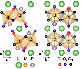
We now turn to a real materials example, and choose the family of lithium transition-metal phosphates, LiMPO4, M = Mn, Fe, Co, Ni, as our model system. All of the LiMPO4 compounds crystallize in the olivine structure with the orthorhombic space group and the crystallographic point group .[25, 26, 27, 28, 29] The lattice parameters and atomic coordinates, obtained from first-principles calculations in this work and Refs. 30 and 31, are given in Table 1.
| Mn | Fe | Co | Ni | |||
|---|---|---|---|---|---|---|
| a (Å) | ||||||
| b/a | ||||||
| c/a | ||||||
| M | x | |||||
| M | z | |||||
| P | x | |||||
| P | z | |||||
| O1 | x | |||||
| O1 | z | |||||
| O2 | x | |||||
| O2 | z | |||||
| O3 | x | |||||
| O3 | y | |||||
| O3 | z |
The transition metal cations occupy the sites with Wyckoff positions ; these are surrounded by strongly distorted oxygen octahedra and have local symmetry. All compounds have a transition to an antiferromagnetic state at some tens of kelvin. The resulting magnetic order breaks the inversion symmetry in all cases and hence allows for the linear magnetoelectric effect. Across the series, however, three distinct antiferromagnetic orderings emerge [32, 33, 28, 34, 35], summarized in Table 2. These different antiferromagnetic orderings lead in turn to different magnetic symmetries and different allowed monopolar contributions.
| Mn | Fe / Co | Ni | |
|---|---|---|---|
| (, 0, 0) | (0, , 0) | (0, 0, ) | |
| (, 0, 0) | (0, , 0) | (0, 0, ) | |
| (, 0, 0) | (0, , 0) | (0, 0, ) | |
| (, 0, 0) | (0, , 0) | (0, 0, ) | |
| () | 5 | 4 / 3 | 2 |
| point group | (M) | (Li) | (O3) | ||||||||||||||
|---|---|---|---|---|---|---|---|---|---|---|---|---|---|---|---|---|---|
| , | , | , | , | ||||||||||||||
| 1 | 1 | 1 | 1 | 1 | 1 | 1 | 1 | 0 | 0 | 0 | 0 | 0 | |||||
| 1 | 1 | -1 | -1 | 1 | 1 | -1 | -1 | 0 | 0 | 0 | 0 | ||||||
| 1 | -1 | 1 | -1 | 1 | -1 | 1 | -1 | 0 | 0 | 0 | 0 | 0 | |||||
| 1 | -1 | -1 | 1 | 1 | -1 | -1 | 1 | 0 | 0 | 0 | 0 | ||||||
| 1 | 1 | 1 | 1 | -1 | -1 | -1 | -1 | 0 | 0 | 0 | |||||||
| 1 | 1 | -1 | -1 | -1 | -1 | 1 | 1 | 0 | 0 | 0 | 0 | ||||||
| 1 | -1 | 1 | -1 | -1 | 1 | -1 | 1 | 0 | 0 | 0 | |||||||
| 1 | -1 | -1 | 1 | -1 | 1 | 1 | -1 | 0 | 0 | 0 | 0 | ||||||
IV.1 Symmetry analysis
In Table 3 we show the character table of the symmetry group and indicate which irreducible representations are adopted by each possible collinear ordering of the transition metal magnetic moments, , along the cartesian axes, as well as the symmetries of the possible monopolar , toroidal and quadrupolar orderings on the transition metal sites.
In LiMnPO4 the easy axis is the axis, and the magnetic moments adopt a C-type antiferromagnetic ordering with order parameter [34], this combination belongs to the irreducible representation of the the symmetry group. (This ordering allows for a simultaneous A-type antiferromagnetic canting along the axis which is negligible in our DFT calculations and we neglect here. Note that a weak ferromagentic canting has also been reported, which is not compatible with the symmetry analysis[36]; this we also neglect.) We see from the line corresponding to the irreducible representation in Table 3 that the ordering of local M-site monopole moments all with the same sign also has symmetry, therefore LiMnPO4 is ferromonopolar and supports a macroscopic monopolization. Conversely there is no net toroidal moment, with only an anti-ferrotorodial ordering along the direction allowed on the Mn sites. This is consistent with the experimental observation that the magnetoelectric response has only diagonal components[37]. We note also that the and quadrupolar components have the same symmetry as the monopole; these quadrupolar contributions are responsible for the inequality between the magnitudes of the diagonal elements of the magnetoelectric tensor.
LiCoPO4 has been of particular recent interest because the observation of ferrotoroidic domains using nonlinear optical techniques has been reported.[3] Both LiCoPO4 and LiFePO4 also adopt a C-type antiferromagnetic ordering, but in contrast to LiMnPO4, both have their easy axis primarily along the axis[38, 33]. This corresponds to the irreducible representation which we see from Table 3 disallows both a macroscopic monopolization and any local monopolar contribution on the transition metal sites. This symmetry allows, however, a toroidal moment parallel to the axis. As a result the magnetoelectric responses of both compounds are entirely off-diagonal[39, 37], although is not exactly equal to - (which would be the case for a purely toroidal response) because a ferroquadrupolar component is allowed with the same symmetry as . (We note that recently it was found that the magnetic moments in LiCoPO4 and LiFePO4 are rotated slightly away from the direction [32, 40]. Such a symmetry lowering is not compatible with the space group and requires an additional structural distortion that has not yet been identified. We do not treat these further symmetry lowerings here.)
Finally we turn to the case of LiNiPO4, which again has C-type AFM ordering, but this time with easy axis along the direction[35], so that the Ni sublattice has magnetic point group and transforms according to the representation. (This symmetry also allows a small A-type AFM canting of the magnetic moments along the direction which has been reported [35] and which we neglect here). While this symmetry does not allow a net macroscopic monopolization, local monopoles are allowed on the Ni ions and must order with an antimonopolar arrangement. A macroscopic toroidal moment is again allowed, this time along the direction, consistent with the corresponding off-diagonal magnetoelectric effect[41, 35, 30].
In this series, therefore, we find one example – LiMnPO4 – of a material with a net monopolization, in which the local monopole moments on the transition metal sites are aligned in a ferromonopolar arrangement. We also find an example – LiNiPO4 – which has no macroscopic monopolization, but has a finite- antimonopolar ordering on the transition metal sites. In the remaining two compounds – LiCoPO4 and LiFePO4 – the macroscopic monopolization and the local monopoles on the transition metal sites are both zero by symmetry. We summarize our symmetry analysis in Table 4.
| label | magnetic order | ME | Toroidal | Monopole | |
|---|---|---|---|---|---|
| Mn | , | ||||
| Co, Fe | 0 | ||||
| Ni | , | 0 |
While it is at first sight tempting to describe LiCoPO4 and LiFePO4 as non-monopolar, this is not strictly correct, as we discuss next. First, we note that in the LiMPO4 family, the P atom and the O1 and O2 atoms also occupy sites, and so follow the same symmetry transformations as the transition metal ions. This means that for LiMnPO4 and LiNiPO4 local monopoles are allowed on these atoms. Of the remaining sites, the of Li have only as a symmetry operation, and the sites of the O3 have no site symmetry. In Table 3 we also list the symmetries and possible monopole orderings of the and sites. We find that for the irreducible representation of LiMnPO4, the monopoles on Li and O3 have the same ferromonopolar ordering as the Mn sites. Likewise, for LiNiPO4, in which the Ni sites have antiferromonopolar ordering, an antiferromonopolar ordering of the Li and O3 monopoles is also found. Most notably, for LiFePO4 and LiCoPO4, which have non-monopolar transition metal sites, antiferromagnetically ordered monopoles are allowed on the and sites.
In the next section we use first-principles density functional theory to calculate the magnitudes of these various contributions.
IV.2 Density functional calculations of atomic site monopoles and macroscopic monopolizations
Our calculations were done using the local spin density approximation with an additional Hubbard correction on the transition metal sites (the LSDA method). We took values of =5eV and =0.75eV for all systems; these values correctly reproduce the experimentally reported magnetic orderings and anisotropies. For structural optimizations we used the Vienna ab initio simulation package (VASP) [42] with a plane-wave basis set and projector augmented wave[43] potentials. Our energy cutoff and -point grid were 500 eV and respectively. We used default VASP PAW potentials with the following electrons in the valence: Li (1s, 2s), O (2s, 2p), P (3s, 3p), Co (3d, 4s), Mn, Fe and Ni (3p, 3d, 4s). Structural relaxations were performed in the absence of spin-orbit coupling. For the monopole calculations we used the structures obtained form the VASP code, then used the linearized augmented plane wave (LAPW) method as implemented in the ELK code[44] with spin-orbit coupling included to calculate the charge and spin density. We used a basis set of , a k-point sampling of the Brillouin zone and took the product of the muffin tin radius and the maximum reciprocal lattice vector to be 7.5. To calculate the atomic site monopoles () we decomposed the the density matrix into tensor moments as described in Section III [16] and evaluated the matrix elements for the transition metal atoms and the matrix elements for the Li, P and O atoms.
In Table 5 we report our calculated local atomic site monopoles , for the series of transition metal phosphates, as well as the local moment contribution, . Note that the orbital component makes no contribution by symmetry to the atomic site monopoles, and its magnitude is negligible in the local moment monopole of the ferromonopolar LiMnPO4 because of the half-filled Mn2+ shell. We also report the total macroscopic monopolizations, normalized to the unit volume, .
The first thing to note is that, in the ferromonopolar case of LiMnPO4, the local moment monopole is as expected considerably larger – by around three orders of magnitude – than the atomic site monopoles. The value of the local moment monopole in one four-formula unit unit cell is 2.09 , whereas the local atomic site monopoles are all around 10. Even when summed over all the atomic sites, the contribution from the atomic site monopoles is still only ; it is so small in part because of cancellations between site monopoles of different sign. The macroscopic monopolization, , which is the total monopole per unit volume, then derives almost entirely from the local moment contribution. We obtain a value of modulo the monopolization increment of . Note that, since we treat the magnetic moments as collinear along a lattice vector there is just one monopolization increment.
For the other compounds a net monopolization is forbidden by symmetry, and so the local moment monopole and the total monopolization are both formally zero. We find, however, non-zero values for those atomic site monopoles that are allowed by symmetry, always with the appropriate symmetry-allowed antiferromagnetic ordering. Particularly interestingly, we find that when atomic site monopoles are symmetry allowed on the P and O atoms, they are comparable to or larger than the values on the transition metals. The relative sizes of the atomic site monopoles can be understood from inspection of the magnetization density: In Fig. 8 we show the isosurface of our calculated magnetization density at 0.00125 for LiNiPO4, with blue and red surfaces indicating positive and negative density, as well as a slice through the magnetization density coinciding with the Ni site positions. The small deviation from a perfectly spherical distribution around the Ni atom is indicative of the monopolar and other non-dipolar multipolar contributions. It is clear that the magnetization density around the oxygen atoms, while smaller in magnitude, is more non-spherical than that around Ni. In particular, the magnetization density changes sign at the O3 sites, indicating a highly non-spherical magnetization density which is consistent with their having the largest atomic site monopoles, The atomic site monopole on Li, although non-zero by symmetry for every case, is always small, consistent with the highly ionic nature of the Li+ ion; since the charge density around the Li ions is close to zero, the magnetization density is too (Fig. 8). Finally we note that the atomic site monopole on Ni in LiNiPO4 is one order of magnitude smaller than that on Mn in LiMnPO4, even though its local magnetic dipole moments is only 2.5 times smaller. Our initial computer experiments suggest that this is partly a result of the different magnetic anisotropy in the two cases, as a calculation with the Ni moments constrained to have the same orientation as those of Mn in LiMnPO4 yields increased atomic site monopoles. A detailed study of the factors that determine the magnitudes of atomic site monopoles will be the subject of future work.

| Mn | Fe | Co | Ni | |
| () | ||||
| M | 1.94 | 0.00 | 0.00 | 0.09 |
| Li | 0.06 | 0.03 | 0.04 | 0.01 |
| P | 3.20 | 0.00 | 0.00 | 0.49 |
| O1 | -7.68 | 0.00 | 0.00 | -3.14 |
| O2 | 7.14 | 0.00 | 0.00 | 4.10 |
| O3 | -1.26 | -6.02 | -6.74 | -7.63 |
| () | 8.52 | 0.00 | 0.00 | 0.00 |
| () | 2091.94 | 0.00 | 0.00 | 0.00 |
| (/Å2) | 6.92 | 0.00 | 0.00 | 0.00 |
| (/Å2) | 5.95 | 0.00 | 0.00 | 0.00 |
V Multiferroic Free Energy with monopole contributions
As stated above, from a macroscopic symmetry point of view, the symmetries which allow for a macroscopic monopolization are identical with that allowing for a diagonal component of the linear magnetoelectric effect tensor. In this section, we develop the relationship between these two quantities by analyzing the following free energy expression:
| (26) |
where and are the electric and magnetic susceptibilities, and are temperature-dependent coefficients, and determines the strength of the magnetoelectric coupling. This is the simplest possible free energy expression that can simultaneously describe (i) a phase transition from a para-monopolar () into a ferromonopolar phase (), (ii) the coupling of the electric polarization and the magnetization to the electric field and the magnetic field , respectively, and (iii) a coupling between the electric polarization, the magnetization, and the monopolization. Note that only the magnetization and the polarization couple to and , the monopolization in general does not couple to any homogeneous external fields, in agreement with the fundamental definitions discussed in Sec. II. The trilinear form of the coupling term in Eq. (26) is the lowest possible order that is compatible with the overall space and time reversal symmetries. Since our purpose here is to discuss the new features arising from this trilinear coupling, we leave for future work the analysis of gradient terms in the free energy that would be required to describe for example variations in monopolization, magnetization or polarization at domain walls. The equilibrium values for and can be obtained by minimizing Eq. (26). This leads to:
| (27) |
and
| (28) |
If one inserts Eq. (28) into Eq. (27) one obtains (to leading order in ):
| (29) |
The last term in Eq. (29) is a symmetric linear magnetoelectric effect proportional to the monopolization. Thus, the presence of the trilinear coupling term between monopolization, magnetization, and polarization in Eq. (26) gives rise to a diagonal magnetoelectric effect in the ferromonopolar phase, with
| (30) |
(Note that an off-diagonal magnetoelectric effect is obtained from a trilinear coupling between toroidization, magnetization and polarization, as discussed in Ref. 4).
Conversely, the presence of a monopolar contribution can be inferred from the existence of a diagonal linear magnetoelectric response, the magnitude of which is determined by the product of the dielectric susceptibility, magnetic permeability, monopolization and the strength of the coupling between , and . If the linear magnetoelectric response is diagonal and isotropic, then there can be no quadrupolar contributions and the response arises entirely from monopolar contributions. We see also from Eqn. 29 that in the case of antiferromonopolar ordering, a homogeneous magnetic field will induce a finite- polarization. Such a relationship could be used in the case of , to provide a more fundamental definition of an antiferroelectric in simultaneously antiferromonopolar systems, than the current unsatisfactory working definition based on the observation of double-loop hysteresis. Finally we mention that an additional interesting consequence of the relationship between the monopolization and the diagonal magnetoelectric effect is the induction of monopoles by electric charge. This has been discussed previously in the context of axion electrodynamics[45], and is currently being revisited in the context of topological insulators[46].
VI Summary, conclusions, and outlook
In summary we have presented a theoretical analysis of magnetoelectric monopoles in bulk periodic solids. We introduced the term “monopolization” to describe the monopole moment per unit volume, and considered two contributions, one arising from the local variation in magnetization density around the atom and the second from the distribution of localized magnetic dipole moments throughout the unit cell. We found that the latter dominates the total monopolization in transition metal compounds with ferromonopolar ordering. We showed that, for ferromonopolar materials, periodic boundary conditions lead to a multivaluedness of the monopolization, suggesting that only differences in monopolization are well-defined observable macroscopic quantities. We found also that care must be taken in evaluating such monopolization differences: For example in the example of the distorted one-dimensional antiferromagnetic chain discussed in Sec.III.3, the change in monopolization due to a structural distortion can be calculated straightforwardly, whereas in the case of a magnetic moment reversal one has to subtract the improper monopolization change that is caused by the corresponding change in the monopolization increment.
Quantitative measurements of monopolizations are challenging. The atomic site monopolization can in principle be detected using resonant x-ray scattering, although the experimental constraints are rather rigorous and a suitable material for such an experiment has not yet been identified. In particular, for most space group symmetries the sites that allow an atomic site monopole also allow an atomic site quadrupolar component, and disentangling the two contributions is not straightforward [18]. This problem can be circumvented by selecting materials with an isotropic diagonal magnetoelectric response [47], however few such materials have been identified to date. Even more problematic is the question of how to measure the macroscopic local moment monopolization. According to the fundamental definition of the monopole moment, this is in principle possible by measuring the effect on a sample of a diverging magnetic field, however such a field is not accessible. It is possible that earlier observations of a quadrupolar magnetic field around a spherical sample of the prototypical diagonal magnetoelectric Cr2O3 [48, 49] also incorporate a monopolar contribution; the theory underlying these measurements will be revisited in future work [50]. It has also been recently proposed that signatures of monopolar behavior will manifest in the transport properties of diagonal magnetoelectrics [51]
An open question, both for ferrotoroidic and ferromonopolar materials is whether the toroidal moment or monopole moment respectively can be a primary order parameter, or is always secondary to an antiferromagnetic or structural ordering. Currently no case has been identified even theoretically in which the monopolization is non-zero while there is no magnetic ordering, although it is possible that some “hidden-order parameter” materials that are of current interest might prove to fall into this class [8]. The fact that the monopole order parameter is a scalar might be helpful in distinguishing responses that arise from the antiferromagnetism from those of the monopole, in cases where the antiferromagnetic order parameter is a vector. Within the class of secondary ferromonopolar materials, it is also an open question whether there is a fundamental difference between the case in which the primary order parameter is the AFM ordering, and that where it is a structural phase transition from a centrosymmetric antiferromagnet (which does not allow monopolization) to a non-centrosymmetric monopolar state.
Finally, we mention that it has been argued that ferrotoroidicity is a key concept for fitting all forms of ferroic order in a simple fundamental scheme based on the different transformation properties of the corresponding order parameters with respect to time and space inversion (see Refs. 1, 2, 3, in particular Fig. 2 in Ref. 3). It is clear that from a symmetry point of view, that the monopolization could play a similar role, since a ferromonopolar material also breaks both space-inversion and time-reversal symmetry. As a result the nonlinear optical techniques used in Ref. 3 to identify ferrotoroidic ordering are sensitive also to the monopolar symmetry breaking, and could provide indirect evidence for the presence of monopolization. In addition, the four fundamental forms of ferroic order, with order parameters transforming according to the four different representations of the “parity group” generated by the two operations of time and space reversal[52] could be chosen to be ferroelasticity, ferroelectricity, ferromagnetism, and ferromonopolicity (rather than ferrotoroidicity). Whether the scalar nature of the monopole, compared with the vector nature of the toroidal moment, makes this choice more or less appropriate is an open question.
Acknowledgements.
This work was supported financially by the ETH Zürich (NAS, MF and EB), by the ERC Advanced Grant program, No. 291151 (NAS and EB), by the Max Rössler Prize of the ETH Zürich (NAS), Nordita (AB), US DoE (AB) and the Swedish Research Council (AB and LN). EB is a Research Associate of the Fonds de la Recherche Scientifique, FNRS, Belgium. NAS thanks Nordita, the Nordic Institute for Theoretical Physics, for their hospitality during a visit where much of this work was performed.References
- [1] H. Schmid, in Introduction to Complex Mediums for Optics and Electromagnetics, edited by W. S. Weiglhoger and A. Lakhtakia (SPIE Press, 2003), pp. 167–195.
- [2] H. Schmid (Kluwer, Dordrecht, 2004), pp. 1–34.
- [3] B. B. V. Aken, J. P. Rivera, H. Schmid, and M. Fiebig, Nature 449, 702 (2007).
- [4] C. Ederer and N. A. Spaldin, Phys. Rev. B 76, 214404 (2007).
- [5] S. W. Lovesey, J. Fernandez-Rodriguez, J. A. Blanco, D. S. Sivia, K. S. Knight, and L. Paolasini, Phys. Rev. B 75, 014409 (2007).
- [6] J. Fernández-Rodríguez, V. Scagnoli, C. Mazzoli, F. Fabrizi, S. W. Lovesey, J. A. Blanco, D. S. Sivia, K. S. Knight, F. de Bergevin, and L. Paolasini, Phys. Rev. B 81, 085107 (2010).
- [7] V. Scagnoli, U. Staub, Y. Bodenthin, R. A. de Souza, M. Garcia-Fernandez, M. Garganourakis, A. T. Boothroyd, D. Prabhakaran, and S. W. Lovesey, Science 332, 696 (2011).
- [8] A. Shekhter and C. Varma, Physical Review B 80, 214501 (2009).
- [9] R. M. C. Castelnovo and S. L. Sondhi, Nature 451, 42 (2008).
- [10] D. J. P. Morris, D. A. Tennant, S. A. Grigera, B. Klemke, C. Castelnovo, R. Moessner, C. Czternasty, M. Meissner, K. C. Rule, J.-U. Hoffmann, et al., Science 326, 411 (2009).
- [11] K. T. Delaney, M. Mostovoy, and N. A. Spaldin, Phys. Rev. Lett. 102, 157203 (2009).
- [12] M. Mostovoy, Phys. Rev. Lett. 96, 067601 (2006).
- [13] H. Katsura, N. Nagaosa, and A. V. Balatsky, Phys. Rev. Lett. 95, 057205 (2005).
- [14] N. A. Spaldin, M. Fiebig, and M. Mostovoy, J. Phys. Condens. Matter 20, 434203 (2008).
- [15] G. van der Laan and B. Thole, J. Phys.: Condens. Matter 7, 9947 (1995).
- [16] F. Bultmark, F. Cricchio, O. Granas, and L. Nordström, Phys. Rev. B 80, 035121 (2009).
- [17] S. W. Lovesey and V. Scagnoli, J. Phys. Condens. Matter 21, 474214 (2009).
- [18] U. Staub, Y. Bodenthin, C. Piamonteze, M. García-Fernández, V. Scagnoli, M. Garganourakis, S. Koohpayeh, D. Fort, and S. W. Lovesey, Phys. Rev. B 80, 140410 (2009).
- [19] P. D. Visschere, J. Phys. D 39, 4278 (2006).
- [20] R. Resta, Eur. Phys. Lett. 22, 133 (1993).
- [21] R. Resta, Rev. Mod. Phys. 66, 899 (1994).
- [22] R. D. King-Smith and D. Vanderbilt, Phys. Rev. B 47, R1651 (1993).
- [23] D. Vanderbilt and R. D. King-Smith, Phys. Rev. B 48, 4442 (1993).
- [24] D. Vanderbilt, J. Phys. Chem. Solids 61, 147 (2000).
- [25] D. Destenay, Mém. Soc. Roy. Sci. Liège 10, 5 (1950).
- [26] R. E. Newnham and M. J. Redman, J. Am. Chem. Soc. 48, 547 (1965).
- [27] S. Geller and J. L. Durand, Acta Cryst. 13, 325 (1960).
- [28] R. P. Santoro and R. E. Newnham, Acta Cryst. 22, 344 (1967).
- [29] I. Abrahams and K. S. Easson, Acta Crystallographica Section C: Crystal Structure Communications 49, 925 (1993).
- [30] E. Bousquet, N. A. Spaldin, and K. Delaney, PRL 106, 107202 (2011).
- [31] A. Scaramucci, E. Bousquet, M. Fechner, M. Mostovoy, and N. A. Spaldin, Phys. Rev. Lett. 109, 197203 (2012).
- [32] D. Vaknin, J. L. Zarestky, L. L. Miller, J.-P. Rivera, and H. Schmid, Phys. Rev. B 65, 224414 (2002).
- [33] G. Liang, K. Park, J. Li, R. E. Benson, D. Vaknin, J. T. Markert, and M. C. Croft, Phys. Rev. B 77, 064414 (2008).
- [34] R. Toft-Petersen, N. H. Andersen, H. Li, J. Li, W. Tian, S. L. Bud’ko, T. B. S. Jensen, C. Niedermayer, M. Laver, O. Zaharko, et al., Phys. Rev. B 85, 224415 (2012), URL http://link.aps.org/doi/10.1103/PhysRevB.85.224415.
- [35] T. Jensen, N. Christensen, M. Kenzelmann, H. Rønnow, C. Niedermayer, N. Andersen, K. Lefmann, J. Schefer, M. von Zimmermann, J. Li, et al., Phys. Rev. B 79, 092412 (2009).
- [36] D. Arčon, A. Zorko, R. Dominko, and Z. Jagličič, Journal Of Physics-Condensed Matter 16, 5531 (2004).
- [37] M. Mercier, J. Gareyte, and E. F. Bertaut, Comptes Rendus Hebdomadaires Des Seances De L Academie Des Sciences Serie B 264, 979 (1967).
- [38] R. P. Santoro, D. J. Segal, and R. E. Newnham, J. Phys. Chem. Solids 27, 1192 (1966).
- [39] M. Mercier, P. Bauer, and B. Fouilleux, Comptes Rendus Hebdomadaires Des Seances De L Academie Des Sciences Serie B 267, 1345 (1968).
- [40] J. Li, V. O. Garlea, J. L. Zarestky, and D. Vaknin, Phys. Rev. B 73, 024410 (2006).
- [41] M. Mercier and P. Bauer, Comptes Rendus Hebdomadaires Des Seances De L Academie Des Sciences Serie B 267, 465 (1968).
- [42] G. Kresse and J. Furthmüller, Phys. Rev. B 54, 11169 (1996).
- [43] G. Kresse and D. Joubert, Phys. Rev. B 59, 1758 (1999).
- [44] http://elk.sourceforge.net.
- [45] F. Wilczek, Phys. Rev. Lett. 58, 1799 (1987), URL http://link.aps.org/doi/10.1103/PhysRevLett.58.1799.
- [46] A. M. Essin, J. E. Moore, and D. Vanderbilt, Phys. Rev. Lett. 102, 146805 (2009), URL http://link.aps.org/doi/10.1103/PhysRevLett.102.146805.
- [47] F. W. Hehl, Y. N. Obukhov, J.-P. Rivera, and H. Schmid, Phys. Rev. A 77, 022106 (2008).
- [48] D. N. Astrov and N. B. Ermakov, Journal of Experimental and Theoretical Physics Letters 59, 297 (1994).
- [49] D. N. Astrov, N. B. Ermakov, A. S. Borovik-Romanov, E. G. Kolevatov, and V. I. Nizhankovskii, Journal of Experimental and Theoretical Physics Letters 63, 745 (1996).
- [50] I. Dzyaloshinskii, Solid State Communications 82, 579 (1992).
- [51] D. Khomskii, Magnetic monopoles and unusual transport effects in magnetoelectrics (2013), preprint.
- [52] E. Ascher, Int. J. Magn. 5, 287 (1974).