Density mapping with weak lensing and phase information
Abstract
The available probes of the large scale structure in the Universe have distinct properties: galaxies are a high resolution but biased tracer of mass, while weak lensing avoids such biases but, due to low signal-to-noise ratio, has poor resolution. We investigate reconstructing the projected density field using the complementarity of weak lensing and galaxy positions. We propose a maximum-probability reconstruction of the 2D lensing convergence with a likelihood term for shear data and a prior on the Fourier phases constructed from the galaxy positions. By considering only the phases of the galaxy field, we evade the unknown value of the bias and allow it to be calibrated by lensing on a mode-by-mode basis. By applying this method to a realistic simulated galaxy shear catalogue, we find that a weak prior on phases provides a good quality reconstruction down to scales beyond , far into the noise domain of the lensing signal alone.
Keywords:
cosmology – large-scale structure of the Universe – gravitational lensing: weak – methods: data analysis.1 Introduction
Weak lensing is a promising cosmological probe, allowing the mass distribution in the Universe to be investigated without assumptions about the dynamics of the baryonic component.
In the pioneering work of Kaiser & Squires (1993) it has been shown that weak lensing can be used to map the distribution of dark matter in galaxy clusters. Following this, several methods for making so-called mass maps have been developed, with much attention given to reconstruction methods such as maximum-likelihood approaches (Bartelmann et al., 1996). However, there is a substantial level of noise in the resulting maps, due to the effect of galaxies having intrinsic ellipticities in addition to the sought-after gravitational shear. Therefore it was immediately realised that the reconstruction methods require smoothing or regularisation (Squires & Kaiser, 1996). A significant proposal in this regard is the Maximum-Entropy method known from image reconstruction studies (Bridle et al., 1998; Seitz et al., 1998; Marshall et al., 2002).
These methods work well when applied to clusters, but the lensing ellipticity measurements of galaxies are still sufficiently noisy that reconstruction of the low contrast large-scale structure is not possible with significant signal-to-noise. In this study we develop a methodology attempting to make maps of the projected density with higher signal-to-noise, by utilising a maximum-probability reconstruction with a physically motivated prior probability term: we will examine the usefulness of using Fourier phase information from the distribution of galaxies in the lensing map area. This is related to other recent methods that use galaxy positions to improve density reconstruction (Simon, 2012) or combine weak lensing and galaxy positions to measure bias (Amara et al., 2012); in our case, we do not need to assume an amplitude for the bias.
The paper is organised as follows. In Section 2 we review the relevant theoretical background, including weak gravitational lensing quantities and the Fourier description of fields. We also emphasise the importance of Fourier phases in mapping cosmological fields. In Section 3 we introduce the maximum-probability method. We define the likelihood and the prior term for our reconstruction method, describe the phase prior in detail, and outline the practical implementation of our method. Section 4 describes the simulated dataset used in the analysis and the results of applying the reconstruction method. Finally, we discuss the implications of our work in Section 5.
2 Theory
2.1 Lensing quantities
Here we briefly discuss the necessary lensing theory; full details can be found in e.g. Bartelmann & Schneider (2001) and Munshi et al. (2008).
The flat perturbed Friedman-Robertson-Walker metric of the standard cosmological model is
| (1) |
where is the usual Newtonian gravitational potential and is the scale factor. The potential is related to the matter density field by Poisson’s equation
| (2) |
where describes the perturbation around the mean density of matter in the Universe.
In this spacetime a lensing potential can be defined as
| (3) |
where is the comoving distance of the source and the integration is along the line of sight, and is the position on the sky. This can be understood as a 2-dimensional projection of the gravitational potential. The way in which an image of a source is distorted when passing through a gravitational field depends on a combination of the second order derivatives of the lensing potential
| (4) |
| (5) |
| (6) |
where is called the convergence, and are the two components of the shear , and denote angular derivatives in the and directions respectively. These quantities are found in the Jacobian matrix
| (7) |
which maps the source plane coordinates to the image plane coordinates
| (8) |
The convergence describes the projection of the overdensity field on the sky
| (9) |
and this projected density is the quantity which we seek to reconstruct as a map.
2.2 Fourier description of fields
In our reconstruction method, we will use a prior term which involves the phase of lensing fields, so here we define the required quantities for this term. A real space field such as can be expanded in a Fourier superposition of plane waves:
| (10) |
The Fourier transform of such a field is complex and is described by an amplitude and phase where
| (11) |
A Gaussian random field will have phases distributed independently11 1 There is a caveat to this statement. For a real valued field , its Fourier modes have to satisfy the Hermitian relation . and uniformly on the interval . The statistical properties of the field are then fully specified by its power spectrum , where denotes an average over all modes at a wavenumber .
However, the phase information contained in the field is interesting for two reasons:
- •
Morphology: in cases where one is interested in a specific realisation of a density field, the phases describe features of its spatial pattern (Chiang, 2001). For instance, one might be examining a region of the Universe where one wants to know the spatial distribution of matter, to understand the relationship between density and astrophysical properties (e.g. star-formation).
- •
Non-gaussianity: due to primordial physics (Komatsu et al., 2009, e.g.) and non-linear evolution on scales probed by weak lensing, the field will have non-zero higher order statistics beyond the power spectrum. This higher order information is encoded in a combination of phase and amplitude of the Fourier transformed field. If we can obtain a full estimate of phase and amplitude, we will be able to extract information about the growth of structure and the early Universe (Watts & Coles, 2003; Chiang et al., 2004).
3 Method
3.1 Maximum-Probability reconstruction
Our reconstruction method seeks to find a hypothesis field which has the maximum probability of accounting for the observed data. We suppose that we have a data vector , which contains estimates of shear from observed galaxy ellipticities. We parameterize the hypothesis field by the values of projected density in a grid of pixels. The best fitting set of parameters is then found by maximising the posterior probability according to Bayes’ theorem
| (12) |
where is the likelihood and is the prior probability. The evidence is useful to compare various models , whereas for a particular model we can simply deal with the proportional term on the right hand side. If we have no knowledge of how the parameters of the model should be distributed, we may assume that all values are equaly likely a priori i.e. the prior distribution is flat. Then and the posterior distribution is found by maximising the likelihood. This is the basis of maximum-likelihood methods.
However, the maximum-likelihood method (Bartelmann et al., 1996) will typically overfit the data by fitting the noise. Due to finite sampling of the shear field at galaxy positions, and further contamination of the signal by galaxy ellipticity noise, the reconstruction methods require smoothing or regularisation (Squires & Kaiser, 1996). We can consider two classes of prior which try to achieve this: informative and uninformative priors, differing in the assumptions which they make about the signal. If the purpose of introducing extra information is to regularise rather than inform an inference we can speak of a weakly informative prior.
Over the past two decades different forms of regularisation have been considered. An important example is the Maximum-Entropy (MaxEnt) regularisation known from image reconstruction (Seitz et al., 1998; Bridle et al., 1998; Marshall et al., 2002) which, while being an uninformative prior, benefitted from inferring information about the correlations in the data (Marshall et al., 2002). In addition, methods have been studied with informative priors; these make some assumptions about the nature of the signal, e.g. Wiener filtering (Hu & Keeton, 2002; Simon et al., 2009; Simon et al., 2012). Here we will consider a maximum probability approach with a weakly informative prior.
3.2 Likelihood
We would like to find a best fit hypothesized model for the convergence, , given a set of shear observations . In the flat sky approximation we can relate the convergence and shear fields most easily in Fourier space (Kaiser & Squires, 1993):
| (13) |
| (14) |
As the field of observations will be limited, a simple application of these transformations introduces edge effects, which we will mitigate by making reconstructions over larger patches than the data (see Section 3.4).
The data vector consists of estimates of the shear components and in each pixel of a 2D grid. These are obtained by averaging over galaxy ellipticities in each pixel, so that the error on the mean shear in a pixel is
| (15) |
where is the intrinsic scatter of shear estimators for galaxies, and the mean number of galaxies in a pixel. This error is approximately Gaussian by the central limit theorem.
If our hypothesised convergence field has corresponding shear pixel values , and the data shear pixel values are , then the likelihood for our hypothesized reconstruction is:
| (16) |
where is the noise covariance matrix. Assuming the noise in each pixel is uncorrelated makes the covariance matrix diagonal and simplifies the likelihood to
| (17) |
This assumption is trivially true for shape noise, which dominates on all scales considered. However, intrinsic correlations between galaxy shapes will introduce non-zero off-diagonal terms in the covariance matrix (Catelan et al., 2001; Hirata & Seljak, 2004).
We turn now to consider the prior term for our maximum-probability reconstruction.
3.3 Phase prior
A prior term that accounts for the claim that galaxies trace mass, even if very poorly, can be achieved by constructing a prediction of the lensing convergence based on galaxy count overdensities
| (18) |
where is the number density of galaxies at position and is the mean number density of galaxies at redshift . We could suppose that the overall matter overdensity , where is the galaxy bias. Then we can project according to Equation 9 to find the count-estimated convergence . For a sample divided into redshift bins the projection becomes
| (19) |
where . It would then be possible to require that the hypothesized final convergence field is close to this , within some tolerance.
However, there is a problem with this approach: the bias is unknown, and the claim of linear bias introduces another assumption into the reconstruction.
An easy way of avoiding this problem is to consider only the information about the phases of the Fourier modes of , neglecting their amplitudes. Figure 1 shows the relation between the phases of the true convergence and count convergence found in DES mock catalogue v4.02 (see Section 4.1).
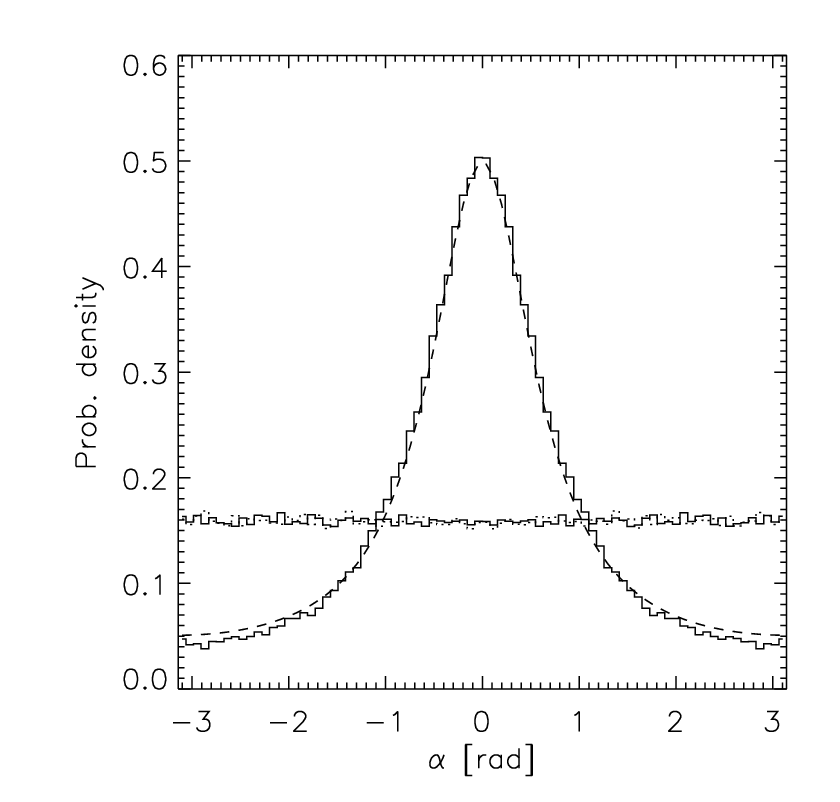
As expected for a close-to-Gaussian field, the histograms of phases for both and fields are close to uniform in the range . However, the overlaid histogram of the phase difference between the true and is visibly spiked around , indicating a strong correlation between the phases of the two fields. We now discuss how this phase difference is calculated in detail.


3.3.1 Phase difference distribution
As the phases are distributed on the interval their differences will have values on the interval . However, since the phases are a cyclic quantity, absolute phase difference will correspond to a phase difference smaller than . This is easily accounted for: if is less than , we add to ; if is greater than or equal to then we subtract from .
We can construct the correlation matrix for the phase difference between true convergence phase and galaxy-count derived convergence phase. In our simulations (Section 4.1), this is constructed from 36 different areas including and information, as for each area only one galaxy distribution realisation is available. By the ergodic principle, this should give an estimate of how much the phases usually differ between the density and galaxy fields in an area. We find that the correlation matrix constructed for pixels is strongly diagonal with the median absolute value of the correlation coefficient .
The histograms of for the whole field (Figure 1) as well as for individal wavenumbers (Figure 2) are well fitted by a wrapped Cauchy probability distribution function:
| (20) |
We note that the distribution is symmetric around zero. The parameter describing the width of the distribution is , where is the half-width of an unwrapped Cauchy distribution. For small values, can be estimated using the median absolute deviation (MAD)
| (21) |
We provide further details on this distribution in Appendix A. However, we want to use the phase information as a weakly informative prior, so we are free to relax this width; we will allow more tolerance in phase difference between our reconstructed and the field by choosing . Using would take us in the direction of a joint reconstruction of the density field from shear and galaxy position data, which is also of interest; some of our runs in Section 4.2 explore this possibility.
It is to be expected that will be a function of , with the phase differences between galaxies and dark matter for large scale modes being more constrained than for small scale ones. We indeed find this to be the case in our simulations, as shown in Figure 3. The phase difference distribution for each also follows a wrapped Cauchy distribution. This distribution is naturally generated when the difference between and comes from a white noise contribution, such as shot-noise, and possibly a further contribution from the stochasticity of the bias relation (Dekel & Lahav, 1999; Manera & Gaztañaga, 2011). Hence, the low modes have smaller phase differences, as this white noise offset is smaller as a proportion of the signal on these scales.
In the mock catalogue the galaxy biasing is roughly linear and deterministic. It could be that the wrapped Cauchy pdf of the phase differences is typical only for this type of bias, but might be quite different for more complex scenarios. Hence, further studie of how the phase difference distribution arises are important. However, as we permit very large errors on the phase difference, moderate deviations from our simulations’ bias model should not change the conclusions of the paper.
In reality, the estimation of will suffer from systematics originating, for example, from an inhomogeneous galaxy survey. These could be mitigated by methods used for the matter power spectrum estimation, where pixels are reweighted to account for the mask (Feldman et al., 1994; Percival et al., 2004). A further systematic will arise from using photometric redshifts to estimate distances (Figure 4). However, this will be mitigated by the fact the convergence is projected; nevertheless, careful tests of this systematic will be necessary.

3.4 Practical implementation
We are now ready to discuss our approach to finding a reconstructed convergence field. Rather than estimating the posterior distribution of our convergence hypotheses, we will seek a maximum a posteriori (MAP) solution. The reconstruction is performed by seeking a that maximises the posterior probability. The posterior pdf will be generally strongly peaked so it is convenient to work with its logarithm
| (22) |
which varies more slowly with the change in .
As the shape of the posterior pdf is generally unknown, we use a simple heuristic optimiser. We use the idea of Simulated Annealing (Kirkpatrick et al., 1983), but replace the usual Metropolis-Hastings sampler (Metropolis et al., 1953; Hastings, 1970) with a Multi Try Metropolis (Liu et al., 2000) one. In each step a set of trial convergence fields is generated from the current field
| (23) |
where components of each are drawn from normal distribution , where the scaling is proportional to the expected signal (see below). A proposal field is then chosen. To limit the random walk behaviour, the field with the highest probability different from the current one is chosen. Then a reference set that includes is formed from that field. The proposal field is then accepted with the probability
| (24) | ||||
| (25) |
In addition to a cooling schedule for the acceptance rate
| (26) |
we have added a similar schedule to decrease the step size in the sampling algorithm
| (27) |
to allow for more refined changes as the optimiser gets closer to the solution we seek (Elson et al., 2007; Kotze, 2009). The solution with the highest probability is stored and used as the output of the optimiser.
Operations on the fields, such as calculating the shears from the convergence, are performed in Fourier space, hence edge effects such as periodic boundaries of the reconstruction will be present. This would mean that the largest scales would not be recovered accurately. This is partially solved by introducing a larger reconstruction grid as suggested in Bridle et al. (1998) and here we use a grid 4 times bigger than the reconstruction area.
To aid the optimisation process we choose a starting position for our hypothesis which is expected to be close to the MAP solution. The initial guess for the reconstruction, , is a field fully consistent with the prior; that is, we choose phases from the galaxy convergence map. We also apply a power spectrum filter to the field
| (28) |
which gives the field the required amplitude of power spectrum and suppresses the high- noise. As this is only a starting guess, any with a very approximately correct shape and amplitude should suffice. Here, we choose the true average power spectrum from simulations. By choosing this starting point, the optimizer evolves the reconstruction from the prior to the posterior under the influence of lensing.
However, to check for possible local maxima in the posterior, we also try running the code from a noisy position such as without applying any filters.
4 Application to simulated data
4.1 Simulated galaxy catalogue

For this study we have used the mock galaxy catalogues created for the Dark Energy Survey based on the algorithm Adding Density Determined GAlaxies to Lightcone Simulations (ADDGALS; Wechsler et al 2013, in preparation; Busha et al 2013, in preparation). This algorithm attaches synthetic galaxies, including multiband photometry, to dark matter particles in a lightcone output from a dark matter -body simulation and is designed to match the luminosities, colors, and clustering properties of galaxies. The catalogue used here was based on a single ‘‘Carmen’’ simulation run as part of the LasDamas of simulations (McBride et al, in preparation)22 2 Further details regarding the simulations can be found at http://lss.phy.vanderbilt.edu/lasdamas/simulations.html. This simulation modeled a flat CDM universe with and in a 1 Gpc/ box with particles. A 220 sq deg light cone extending out to was created by pasting together 40 snapshot outputs.
The galaxy distribution for this mock catalogue was created by first using an input luminosity function to generate a list of galaxies, and then adding the galaxies to the dark matter simulation using an empirically measured relationship between a galaxy’s magnitude, redshift, and local dark matter density, – the probability that a galaxy with magnitude and redshift resides in a region with local density . This relation was tuned using a high resolution simulation combined with the SubHalo Abundance Matching technique that has been shown to reproduce the observed galaxy 2-point function to high accuracy (Kravtsov et al., 2004; Conroy et al., 2006; Reddick et al., 2012).
For the galaxy assignment algorithm, we choose a luminosity function that is similar to the SDSS luminosity function as measured in Blanton et al. (2003), but evolves in such a way as to reproduce the higher redshift observations (e.g., SDSS-Stripe 82, AGES, GAMA, NDWFS and DEEP2). In particular, and are varied as a function of redshift in accordance with the recent results from GAMA (Loveday et al., 2012).
Once the galaxy positions have been assigned, photometric properties are added. Here, we use a training set of spectroscopic galaxies taken from SDSS DR5. For each galaxy in both the training set and simulation we measure , the distance to the 5th nearest galaxy on the sky in a redshift bin. Each simulated galaxy is then assigned an SED based on drawing a random training-set galaxy with the appropriate magnitude and local density, k-correcting to the appropriate redshift, and projecting onto the desired filters. When doing the color assignment, the likelihood of assigning a red or a blue galaxy is smoothly varied as a function of redshift in order simultaneously reproduce the observed red fraction at low and high redshifts as observed in SDSS and DEEP2.
For the simulation of gravitational lensing, weak lensing shear at each galaxy position was computed using the multiple plane ray tracing code CALCLENS (Becker, 2012). Then an intrinsic ellipticity is assigned to each galaxy. The intrinsic shape distribution and dispersion in these simulations are magnitude dependent and are modeled after those found in deep SuprimeCam i′-band data with excellent seeing (), with fainter galaxies having a higher intrinsic ellipticity dispersion. Averaged over all galaxies .


4.2 Results
| Posterior | Phases tolerance | |
|---|---|---|
| Filt. | ||
| Filt. | ||
| Filt. | ||
| Noisy | ||
| Filt. |
From the simulated catalogue described in Section 4.1, we select a large square square patch of . To study the behaviour of the reconstructions, areas (with replacement) of were randomly selected from this patch. These were divided into pixels of containing galaxies. Hence the number density of sources is . We use the same galaxies as sources and tracers of the density field.
The reconstruction code was run for 30,000 trial steps for each sub-field, with trial fields generated in each optimization step. The reconstructed maps span , containing 14,400 pixels of ; i.e. we reconstruct a larger patch than the data patch in each case.
The reconstructions were performed for each of the fields using different phase distribution parameters and initial guesses that are summarised in Table 1. Using 100 different fields allowed us to examine the noise properties of the reconstruction method.
Reconstructions were performed using a maximum-likelihood (ML) method (i.e. no prior terms) and the maximum-probability approach with the phase prior. In this set of runs, the phase prior included a phase tolerance in order to provide a weakly informative prior. To obtain a reasonable starting point, was filtered according to equation (28).
Figure 5 shows examples of maps obtained using both methods of reconstruction (b and c) with the true simulated convergence map (a) and the convergence estimated from galaxy positions (d) shown for comparison (using , i.e. , see Section 3.3). The ML method reconstructs only the most prominent peaks, with a high level of contamination by spurious peaks. The inclusion of the phases prior appears to improve the map considerably, but it also maps features from that are not necessarily present in the true convergence, e.g. . However, these are consistent with the lensing only reconstruction.
To quantify the quality of the reconstruction, we construct a power spectrum of the error per mode in the reconstruction,
| (29) |
A faithful reconstruction will have small , preferably smaller than the true power in order to achieve good (i.e. the errors in the reconstruction are preferably smaller than the signal of the reconstructed structures for a given scale). shows the scale dependence of the reconstruction faithfulness. However, it is not intended as a metric of how well we can reconstruct the power spectrum from the maps.
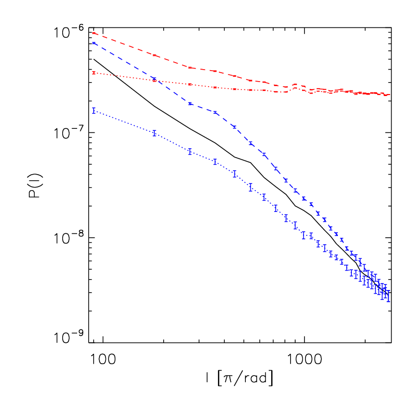


Figure 6 shows the power spectra (dashed) and error power spectra (dotted) of the reconstruction averaged over fields. The maximum-likelihood reconstruction (red) is dominated by noise on most scales. Including the phase prior (blue) leads to a reconstruction that has higher than the ML reconstruction on all scales, and has even beyond , far into the domain where the initial shear data is noise-dominated. On a pixel by pixel basis the phase prior improves the correlation between the true convergence and the reconstruction as shown in Figure 7. The Pearson correlation coefficient changes from for the ML reconstruction to in the case of the MP reconstruction.
The reduction of the noise visible in Figure 6 is due to the interplay between the galaxy phases and both the phase and amplitude of the lensing. Given noisy shear data, and if the phases of the two fields disagree strongly, the only permitted hypothesis that satisfies both the phase prior and the likelihood with modest probability, has low amplitude for the signal. On the other hand, where the phases agree, a higher amplitude is permitted.
To assess the errors on curves in Figure 6, an additional runs different starting points were performed on a single field, to see the variation in reconstructions permitted by the optimiser. The different fields were generated by multiplying each mode in by a complex random number with each component drawn from a standard normal distribution . The error bars on different power spectra in Figures 6, 8 and 9 show the standard deviation in error powers of this set of runs. We see that these errors are substantially smaller than the variation between the maximum-likelihood and maximum-probability runs (Figure 6) and also between maximum-probability runs with different values of the parameter (Figure 9).
To check the dependence of the reconstruction on the initial guess , further reconstructions with the phase prior were performed. The phase tolerance was again set to but was left unfiltered. Figure 8 shows the errors on these reconstruction compared to the analogous filtered one. The reconstruction with an unfiltered starting guess (green dotted) deviates more from the reconstruction with a filtered one (blue dashed) on small scales, suggesting that the posterior probability surface is very flat in some directions (or multimodal). Although, the difference is visible on all scales, the reconstruction remains a substantial improvement over the maximum likelihood reconstruction in Figure 6.
The tolerance we permit on the phases has a moderate impact on the reconstruction, as shown in Figure 9. The lines show error power spectra for reconstruction with phase tolerance of (red dotted), (green dashed) and (blue dot-dashed), and the error power grows by a factor of two on intermediate scales between the tightest and weakest of these tolerances. However, independent of the phase tolerance the reconstructions are similar on small scales where the reconstruction is noise dominated, and on the largest scales where the likelihood term is large.
5 Conclusions
In this paper, we have proposed a maximum-probability reconstruction method for the lensing convergence, and have studied the impact of a physically motivated prior term.
To put a weakly informative prior on the Fourier phases of the modes, we made a prediction of the convergence from the galaxy number overdensity, and used this to inform the preferred phases of the reconstructed convergence field. In this way, by using only the phases of this field, we avoid the use of the unknown amplitude of the linear galaxy bias. We also do not require a deterministic bias, as we allow a phase deviation between the galaxy distribution and the underlying matter density.
By implementing and testing this method with a realistic simulated galaxy shear catalogue, we have found that a weak prior on phases provides a good quality 2-D density reconstruction with signal-to-noise on scales up to and beyond (Figure 6).
The sensitivity of the phase prior reconstruction to initial conditions (Figure 8) shows that the probability surface is flat in directions associated with noise dominated modes, as expected. However, an approximate knowledge of the power spectrum can help to select a solution with modest signal-to-noise even on the smallest scales. The phase difference tolerance can be made more or less strict, depending on whether one wishes to make a joint reconstruction using weak lensing and phases, or instead to make a reconstruction from weak lensing weakly informed by phases. In either case, the reconstruction is found to be an improvement over maximum likelihood reconstruction (contrast Figures 9 and 6).
Although, most of the phase information is coming from the galaxy field, the amplitude of the modes is determined by the interplay between these and the lensing, which includes both phase and amplitude information. It is important to emphasise that in Figure 5(d) the amplitude is an assumption, whereas in Figure 5(c) it is derived purely from data.
In summary, using the phase information from the galaxy distribution to inform weak lensing density reconstruction, appears to be a very powerful addition to the tools we can use for mass mapping. As these maps combine information from the weak lensing and galaxy fields, they can potentially be used to improve our understanding of the relation between dark matter and galaxies, i.e. the bias.
Acknowledgments
We thank Bruce Bassett, Mathew Becker, Rob Crittenden, Alan Heavens and Phil Marshall for useful discussions. RS also thanks B. Bassett for organising the Cape Town Cosmology School 2012 which inspired some of the ideas presented in this paper.
This work was partially supported by STFC grant ST/K00090X/1 and a Royal Society-NRF International Exchange Grant. RS acknowledges support from STFC in the form of a Research Studentship. PM is supported by the U.S. Department of Energy under Contract No. DE- FG02-91ER40690.
Please contact the authors to request access to research materials discussed in this paper.
References
- Amara et al. (2012) Amara A. et al., 2012, MNRAS, 424, 553
- Bartelmann et al. (1996) Bartelmann M., Narayan R., Seitz S., Schneider P., 1996, ApJ, 464, L115+
- Bartelmann & Schneider (2001) Bartelmann M., Schneider P., 2001, Phys. Rep., 340, 291
- Becker (2012) Becker M. R., 2012, arXiv:1210.3069
- Blanton et al. (2003) Blanton M. R. et al., 2003, ApJ, 592, 819
- Bridle et al. (1998) Bridle S. L., Hobson M. P., Lasenby A. N., Saunders R., 1998, MNRAS, 299, 895
- Catelan et al. (2001) Catelan P., Kamionkowski M., Blandford R. D., 2001, MNRAS, 320, L7
- Chiang (2001) Chiang L.-Y., 2001, MNRAS, 325, 405
- Chiang et al. (2004) Chiang L.-Y., Naselsky P. D., Coles P., 2004, ApJ, 602, L1
- Conroy et al. (2006) Conroy C., Wechsler R. H., Kravtsov A. V., 2006, ApJ, 647, 201
- Dekel & Lahav (1999) Dekel A., Lahav O., 1999, ApJ, 520, 24
- Elson et al. (2007) Elson E. C., Bassett B. A., van der Heyden K., Vilakazi Z. Z., 2007, A&A, 464, 1167
- Feldman et al. (1994) Feldman H. A., Kaiser N., Peacock J. A., 1994, ApJ, 426, 23
- Hastings (1970) Hastings W. K., 1970, Biometrika, 57, 97
- Hirata & Seljak (2004) Hirata C. M., Seljak U., 2004, Phys. Rev. D, 70, 063526
- Hu & Keeton (2002) Hu W., Keeton C. R., 2002, Phys. Rev. D, 66, 063506
- Kaiser & Squires (1993) Kaiser N., Squires G., 1993, ApJ, 404, 441
- Kirkpatrick et al. (1983) Kirkpatrick S., Gelatt C. D., Vecchi M. P., 1983, Science, 220, 671
- Komatsu et al. (2009) Komatsu E. et al., 2009, in Astronomy, Vol. 2010, astro2010: The Astronomy and Astrophysics Decadal Survey, p. 158
- Kotze (2009) Kotze J., 2009, PhD thesis, University of Cape Town, Cape Town, ZA
- Kravtsov et al. (2004) Kravtsov A. V., Berlind A. A., Wechsler R. H., Klypin A. A., Gottlöber S., Allgood B., Primack J. R., 2004, ApJ, 609, 35
- Liu et al. (2000) Liu J. S., Liang F., Wong W. H., 2000, JASA, 95, pp. 121
- Loveday et al. (2012) Loveday J. et al., 2012, MNRAS, 420, 1239
- Manera & Gaztañaga (2011) Manera M., Gaztañaga E., 2011, MNRAS, 415, 383
- Marshall et al. (2002) Marshall P. J., Hobson M. P., Gull S. F., Bridle S. L., 2002, MNRAS, 335, 1037
- Metropolis et al. (1953) Metropolis N., Rosenbluth A. W., Rosenbluth M. N., Teller A. H., Teller E., 1953, The Journal of Chemical Physics, 21, 1087
- Munshi et al. (2008) Munshi D., Valageas P., van Waerbeke L., Heavens A., 2008, Phys. Rep., 462, 67
- Percival et al. (2004) Percival W. J., Verde L., Peacock J. A., 2004, MNRAS, 347, 645
- Reddick et al. (2012) Reddick R. M., Wechsler R. H., Tinker J. L., Behroozi P. S., 2012, arXiv:1207.2160
- Seitz et al. (1998) Seitz S., Schneider P., Bartelmann M., 1998, A&A, 337, 325
- Simon (2012) Simon P., 2012, arXiv:1203.6205
- Simon et al. (2012) Simon P. et al., 2012, MNRAS, 419, 998
- Simon et al. (2009) Simon P., Taylor A. N., Hartlap J., 2009, MNRAS, 399, 48
- Squires & Kaiser (1996) Squires G., Kaiser N., 1996, ApJ, 473, 65
- Watts & Coles (2003) Watts P., Coles P., 2003, MNRAS, 338, 806
Appendix A Wrapped Cauchy distribution
The Cauchy pdf is given by
| (30) |
The Wrapped Cauchy pdf is defined as
| (31) |
which gives
| (32) |
where and .
A Cauchy distributed random number can be generated from two independent normally distributed random numbers as
| (33) |
Then a Wrapped Cauchy distributed random number is obtained by taking
| (34) |
and applying a procedure similar to the one in Section 3.3.1, i.e., if is less than , we add to ; if is greater than or equal to then we subtract from .
For a distribution with the parameter can be approximated (for small values) as (Figure 10). For high values of this approximation breaks down; as the Wrapped Cauchy tends to a uniform distribution, and goes to a constant equal to the standard deviation of the uniform distribution, here (see Figure 10).