跳到论文正文
W Papers独立论文阅读器 arXiv:1306.5266 论文正文 计算阅读时间 · 0%
引用这篇论文根据当前论文元数据生成,正式投稿前建议核对。


License: arXiv.org perpetual non-exclusive license
arXiv:1306.5266v2 [math.PR] 07 Nov 2013

On large deviations for the cover time of two-dimensional torus

Francis Comets    Christophe Gallesco    Serguei Popov    Marina Vachkovskaia
Abstract

Let 𝒯n{\mathcal{T}}_{n} be the cover time of two-dimensional discrete torus ℤn2=ℤ2/n​ℤ2{\mathbb{Z}}^{2}_{n}={\mathbb{Z}}^{2}/n{\mathbb{Z}}^{2}. We prove that ℙ[𝒯n≤4πγn2ln2n]=exp(−n2​(1−γ)+o​(1))\mathbb{P}[{\mathcal{T}}_{n}\leq\frac{4}{\pi}\gamma n^{2}\ln^{2}n]=\exp(-n^{2(1-\sqrt{\gamma})+o(1)}) for γ∈(0,1)\gamma\in(0,1). One of the main methods used in the proofs is the decoupling of the walker’s trace into independent excursions by means of soft local times.
Keywords: soft local time, hitting time, simple random walk
AMS 2000 subject classifications: Primary 60G50, 82C41. Secondary 60G55.

1{}^{~1}Université Paris Diderot – Paris 7, Mathématiques, case 7012, F–75205 Paris Cedex 13, France
e-mail: comets@math.univ-paris-diderot.fr

2{}^{~2}Department of Statistics, Institute of Mathematics, Statistics and Scientific Computation, University of Campinas – UNICAMP, rua Sérgio Buarque de Holanda 651, 13083–859, Campinas SP, Brazil
e-mails: {gallesco,popov,marinav}@ime.unicamp.br

1 Introduction and results

Let (Xt,t=1,2,3,…)(X_{t},t=1,2,3,\ldots) be a discrete-time simple random walk on the two-dimensional discrete torus ℤn2=ℤ2/n​ℤ2{\mathbb{Z}}^{2}_{n}={\mathbb{Z}}^{2}/n{\mathbb{Z}}^{2}. Define the entrance time to the site x∈ℤn2x\in{\mathbb{Z}}^{2}_{n} by

Tn​(x)=min⁡{t≥0:Xt=x},T_{n}(x)=\min\{t\geq 0:X_{t}=x\}, (1.1)

and the cover time of the torus by

𝒯n=maxx∈ℤn2⁡Tn​(x),{\mathcal{T}}_{n}=\max_{x\in{\mathbb{Z}}^{2}_{n}}T_{n}(x), (1.2)

that is, 𝒯n{\mathcal{T}}_{n} is the first instant of time when all the sites of the torus were already visited by the walk.

The analysis of cover time by the planar random walk was suggested in [17] under the picturesque name of “white screen problem”, and was soon after popularized in the probabilistic community [1, Chapter 7]. We refer to [5] for a substantial survey on cover times, and to [16] for a short account with a focus on exceptional points. Besides being an appealing fundamental question, the study of cover time is of primer interest for performance evaluation of broadcast procedures in random networks, see e.g. [11].

Not only natural, the two-dimensional model is also more difficult than its higher-dimensional counterparts. This is because dimension two is critical for the walk, resulting in strong correlations. To illustrate the dimension-based comparison, observe that very fine results are available for d≥3d\geq 3, see e.g. [2] and references therein, and also [10] where a closely related continuous problem was studied. In contrast, in two dimensions the first-order asymptotics of the cover time was completed only recently, after a series of intermediate steps over a decade of efforts. In [6] it was proved that

𝒯nn2​ln2​n→4π​ in probability, as n→∞.\frac{{\mathcal{T}}_{n}}{n^{2}\ln^{2}n}\to\frac{4}{\pi}\text{ in probability, as $n\to\infty$}. (1.3)

More rough results, without the precise constant, can be obtained using the Matthews’ method [14]. The result (1.3) was then refined in [8]; in the same paper it was suggested that 𝒯n/2​n2\sqrt{{\mathcal{T}}_{n}/2n^{2}} should be around 2/π​ln⁡n−c​ln⁡ln⁡n\sqrt{2/\pi}\ln n-c\ln\ln n for a positive constant cc (observe that (1.3) means that 𝒯n/2​n2=(2/π+o⁡(1))​ln⁡n\sqrt{{\mathcal{T}}_{n}/2n^{2}}=\big(\sqrt{2/\pi}+o(1)\big)\ln n). This can be seen as a step towards the conjecture of [4] that 𝒯n/n2\sqrt{{\mathcal{T}}_{n}/n^{2}} should be tight around its median and nondegenerate. Such fine properties should be related to the fine structure of late points of the walk, i.e., the sites that get covered only “shortly” before 𝒯n{\mathcal{T}}_{n}. In spite of a very significant progress on this question achieved in [7], much remains to be discovered.

Now, we formulate our result on the deviations from below for the cover time:

Theorem 1.1.

Assume that γ∈(0,1)\gamma\in(0,1). Then, for all ε>0\varepsilon>0 we have

exp(−n2​(1−γ)+ε)≤ℙ[𝒯n≤4πγn2ln2n]≤exp(−n2​(1−γ)−ε)\exp\big(-n^{2(1-\sqrt{\gamma})+\varepsilon}\big)\leq\mathbb{P}\Big[{\mathcal{T}}_{n}\leq\frac{4}{\pi}\gamma n^{2}\ln^{2}n\Big]\leq\exp\big(-n^{2(1-\sqrt{\gamma})-\varepsilon}\big) (1.4)

for all large enough nn.

It should be mentioned that in [3] it was proved that it is exponentially unlikely to cover any bounded degree graph in linear (with respect to the number of vertices) number of steps. In this paper, however, we are concerned with times which differ from the cover time only by a constant factor, and so we obtain only stretched exponential decay.

Remark 1.2.

In fact, in Section 3.1 we prove a bit more than the upper bound in (1.4). Namely, assume that γ∈(0,1)\gamma\in(0,1), fix an arbitrary α∈(γ,1)\alpha\in(\sqrt{\gamma},1) and tile the torus ℤn2{\mathbb{Z}}^{2}_{n} with boxes of size nαn^{\alpha}. Then there exist c=c⁡(α,γ)>0c=c(\alpha,\gamma)>0, c′=c′​(α,γ)>0c^{\prime}=c^{\prime}(\alpha,\gamma)>0, such that, at the moment 4π​γ​n2​ln2​n\frac{4}{\pi}\gamma n^{2}\ln^{2}n, there are at least c​n2​(1−α)cn^{2(1-\alpha)} boxes which are not completely covered, with probability at least 1−exp⁡(−c′​n2​(1−α))1-\exp(-c^{\prime}n^{2(1-\alpha)}).

For completeness, we also include the result on the deviations from the other side:

Theorem 1.3.

Assume that γ>1\gamma>1. Then, for all ε>0\varepsilon>0 we have

n−2​(γ−1)−ε≤ℙ[𝒯n≥4πγn2ln2n]≤n−2​(γ−1)+εn^{-2(\gamma-1)-\varepsilon}\leq\mathbb{P}\Big[{\mathcal{T}}_{n}\geq\frac{4}{\pi}\gamma n^{2}\ln^{2}n\Big]\leq n^{-2(\gamma-1)+\varepsilon} (1.5)

for all large enough nn.

However, it should be noted that the proof of Theorem 1.3 is not difficult once one has (1.3), although, to the best of our knowledge, it did not appear in the literature explicitly in this form.

To see how the proof of Theorem 1.3 can be obtained, observe first that we have for all β>0\beta>0, ε>0\varepsilon>0, all large enough nn and all x∈ℤn2x\in{\mathbb{Z}}^{2}_{n},

maxy∈ℤn2ℙy[Tn(x)≥2πβn2ln2n]\displaystyle\max_{y\in{\mathbb{Z}}^{2}_{n}}\mathbb{P}_{y}\Big[T_{n}(x)\geq\frac{2}{\pi}\beta n^{2}\ln^{2}n\Big] ≤n−β+ε,\displaystyle\leq n^{-\beta+\varepsilon}, (1.6)
miny∈ℤn2y≠xℙy[Tn(x)≥2πβn2ln2n]\displaystyle\min_{\begin{subarray}{c}y\in{\mathbb{Z}}^{2}_{n}\\ y\neq x\end{subarray}}\mathbb{P}_{y}\Big[T_{n}(x)\geq\frac{2}{\pi}\beta n^{2}\ln^{2}n\Big] ≥n−β−ε.\displaystyle\geq n^{-\beta-\varepsilon}. (1.7)

The estimate (1.6) is Lemma 3.3 of [7]; in fact, it is straightforward to modify the proof of the same lemma to obtain (1.7).

Now, the second inequality in (1.5) immediately follows from (1.6) and the union bound. As for the first inequality, the strategy for achieving this lower bound can be described in the following way: let the random walk evolve freely almost up to the expected cover time so that, with good probability there are still uncovered sites, and then choose any particular uncovered site and make the walk avoid it till the end. More precisely, observe that, by (1.3), for any fixed δ>0\delta>0 it holds that

ℙ[𝒯n≥4π(1−δ)n2ln2n]≥12\mathbb{P}\Big[{\mathcal{T}}_{n}\geq\frac{4}{\pi}(1-\delta)n^{2}\ln^{2}n\Big]\geq\frac{1}{2}

for all nn large enough; that is, at time 4π​(1−δ)​n2​ln2​n\frac{4}{\pi}(1-\delta)n^{2}\ln^{2}n there is at least one uncovered site with probability at least 12\frac{1}{2}. An application of (1.7) with β=2​(γ−1+δ)\beta=2(\gamma-1+\delta) concludes the proof of Theorem 1.3.

One can informally interpret (1.6)–(1.7) in the following way: hitting time of a fixed state has approximately exponential distribution with mean 2π​n2​ln⁡n\frac{2}{\pi}n^{2}\ln n. First, the convergence in (1.3) agrees with the intuitive understanding that “hitting times of different sites should be roughly independent”, since the maximum of n2n^{2} i.i.d. exponential random variables with mean 2π​n2​ln⁡n\frac{2}{\pi}n^{2}\ln n is concentrated around 4π​n2​ln2​n\frac{4}{\pi}n^{2}\ln^{2}n. Moreover, the probability for the maximum of such r.v.’s to be larger by a factor γ>1\gamma>1 than this value is n−2​(γ−1)+o​(1)n^{-2(\gamma-1)+o(1)}. It is interesting to observe that, while Theorem 1.3 still agrees with this intuition, Theorem 1.1 does not. Indeed, the probability that the maximum of n2n^{2} i.i.d. exponential random variables with mean 2π​n2​ln⁡n\frac{2}{\pi}n^{2}\ln n is at most 4π​γ​n2​ln2​n\frac{4}{\pi}\gamma n^{2}\ln^{2}n (where γ∈(0,1)\gamma\in(0,1)) is of order (1−n2​γ)n2≃exp⁡(−n2​(1−γ))(1-n^{2\gamma})^{n^{2}}\simeq\exp(-n^{2(1-\gamma)}), which is not the actual order of magnitude obtained in Theorem 1.1. Thus, the behavior of the lower tails of the cover time reveals the fine dependence between hitting times of the different points on the torus.

To prove the upper bound in (1.4), we use the method of soft local times initially developed in [15], where it was used to obtain strong decoupling inequalities for the traces left by random interlacements on disjoint sets. This approach allows to simulate an adapted process on a general space Σ\Sigma using a realization of a Poisson point process on Σ×ℝ+\Sigma\times{\mathbb{R}}_{+}. Naturally, one can use the same realization of the Poisson process to simulate several different processes on Σ\Sigma, thus giving rise to a coupling of these processes. We do this to compare the excursions of the random walk at different regions with the independent excursions, that is, in some sense, we decouple the traces of the random walk in different places, which of course makes things simpler.

Let us comment also on the large deviations for the cover time of the torus in dimension d≥3d\geq 3. This question was studied in [10] in the continuous setting, i.e., for the Brownian motion. Among other results, in [10] the many-dimensional counterparts of Theorems 1.1 (only the upper bound, by exp⁡(−nd⁡(1−γ)+o⁡(1))\exp(-n^{d(1-\gamma)+o(1)})) and (1.3) were obtained. We expect no substantial difficulties in obtaining the same results for the random walk using the same methods as in the present paper, except for the lower bound for the deviation probability from below, since the approach of Section 3.2 fails in higher dimensions.

Notational convention: in the case when the starting point of the random walk is fixed, we indicate that in the subscript; otherwise, the initial distribution of the random walk is considered to be uniform. The positive constants (not depending on nn but possibly depending on the quantities, such as γ\gamma in Theorem 1.1, which are considered to be fixed) are denoted by c,c′,c1,c3,c4c,c^{\prime},c_{1},c_{3},c_{4} etc. Also, it is convenient to view the random walks on the torus, simultaneously for all torus sizes nn, as the random walk on the full lattice observed modulo n​ℤ2n{\mathbb{Z}}^{2}.

2 Soft local times

In this section we describe the method of soft local times [15], which is the key to the upper bound in (1.4).

First, we define the entrance time to a set A⊂ℤn2A\subset{\mathbb{Z}}^{2}_{n} by

Tn​(A)=minx∈A⁡Tn​(x).T_{n}(A)=\min_{x\in A}T_{n}(x).

We write x∼yx\sim y if xx and yy are neighbors in the graph ℤn2{\mathbb{Z}}^{2}_{n}. For A⊂ℤn2A\subset{\mathbb{Z}}^{2}_{n} let us define the (inner) boundary of AA by ∂A={x∈A: there exists ​y∉A​ such that ​x∼y}\partial A=\{x\in A:\text{ there exists }y\notin A\text{ such that }x\sim y\}.

Next, for A⊂ℤn2A\subset{\mathbb{Z}}^{2}_{n} we define the entrance law to AA: for x∉Ax\notin A and y∈∂Ay\in\partial A let

HA(x,y)=ℙx[XTn​(A)=y].H_{A}(x,y)=\mathbb{P}_{x}[X_{T_{n}(A)}=y]. (2.1)

Let us now describe the method of soft local times, which allows us to compare excursions of the random walk with independent excursions. Let A1,…,Ak0,A1′,…,Ak0′⊂ℤn2A_{1},\ldots,A_{k_{0}},A^{\prime}_{1},\ldots,A^{\prime}_{k_{0}}\subset{\mathbb{Z}}^{2}_{n} be such that Aj⊂Aj′A_{j}\subset A^{\prime}_{j}, Aj∩∂Aj′=∅A_{j}\cap\partial A^{\prime}_{j}=\emptyset for j=1,…,k0j=1,\ldots,k_{0}, and Ai′∩Aj′=∅A^{\prime}_{i}\cap A^{\prime}_{j}=\emptyset for i≠ji\neq j. Let A=⋃j=1k0AjA=\bigcup_{j=1}^{k_{0}}A_{j} and A′=⋃j=1k0Aj′A^{\prime}=\bigcup_{j=1}^{k_{0}}A^{\prime}_{j}; and assume that ∂A′=⋃j=1k0∂Aj′\partial A^{\prime}=\bigcup_{j=1}^{k_{0}}\partial A^{\prime}_{j}, which implies also that ∂A=⋃j=1k0∂Aj\partial A=\bigcup_{j=1}^{k_{0}}\partial A_{j}.

Now, suppose that we are only interested in the trace left by the random walk on the set AA. Then, (apart from the initial piece of the trajectory until hitting ∂A′\partial A^{\prime} for the first time) it is enough to know what are the excursions of the random walk between the boundaries of AA and A′A^{\prime}. To define these excursions, consider the following sequence of stopping times:

D0\displaystyle D_{0} =Tn​(∂A′),\displaystyle=T_{n}(\partial A^{\prime}),
S1\displaystyle S_{1} =min⁡{t>D0:Xt∈∂A},\displaystyle=\min\{t>D_{0}:X_{t}\in\partial A\},
D1\displaystyle D_{1} =min⁡{t>S1:Xt∈∂A′},\displaystyle=\min\{t>S_{1}:X_{t}\in\partial A^{\prime}\},

and

Sk\displaystyle S_{k} =min⁡{t>Dk−1:Xt∈∂A},\displaystyle=\min\{t>D_{k-1}:X_{t}\in\partial A\},
Dk\displaystyle D_{k} =min⁡{t>Sk:Xt∈∂A′},\displaystyle=\min\{t>S_{k}:X_{t}\in\partial A^{\prime}\},

for k≥2k\geq 2.

We denote by Σj\Sigma_{j} the space of excursions between ∂Aj\partial A_{j} and ∂Aj′\partial A^{\prime}_{j}; i.e., an element ZZ of this space is a finite nearest-neighbor trajectory beginning at a site of ∂Aj\partial A_{j} and ending on its first visit to ∂Aj′\partial A^{\prime}_{j}. Denote also Σ=⋃j=1k0Σj\Sigma=\bigcup_{j=1}^{k_{0}}\Sigma_{j}. The method of soft local times, as presented in [15], provides a way of constructing the excursions between ∂A\partial A and ∂A′\partial A^{\prime} of the walk XX using a Poisson point process on Σ×ℝ+\Sigma\times{\mathbb{R}}_{+}. To keep the presentation more clear and visual, we use another (in this case, equivalent) way of describing this approach, through a marked Poisson process on ∂A×ℝ+\partial A\times{\mathbb{R}}_{+}.

Refer to caption
Figure 1: The construction of the excursions, the points are represented with crosses, the marks are pictured above them. Observe that we take the initial excursion (up to time D0D_{0}) out of consideration (even if X0∈AX_{0}\in A).

Denote by Zi=(XSi,…,XDi)Z_{i}=(X_{S_{i}},\ldots,X_{D_{i}}) the iith excursion of XX between ∂A\partial A and ∂A′\partial A^{\prime}. According to Section 4 of [15], one can simulate the sequence of excursions (Zi,i=1,2,3,…)(Z_{i},i=1,2,3,\ldots) in the following way, see Figure 1:

  • •

    Consider a marked Poisson point process of rate 11 (with respect to (counting measure on ∂A\partial A)×\times(Lebesgue measure on ℝ+{\mathbb{R}}_{+})) on ∂A×ℝ+\partial A\times{\mathbb{R}}_{+}, with independent marks.

  • •

    These marks are the excursions of the simple random walk starting at the corresponding site of ∂A\partial A and stopped at the first visit to ∂A′\partial A^{\prime}.

  • •

    At time D0D_{0} take ξ0>0\xi_{0}>0 such that there is exactly one point of the Poisson process on the graph of ξ0​HA​(x0,⋅)\xi_{0}H_{A}(x_{0},\cdot) and nothing below this graph, where x0=XD0x_{0}=X_{D_{0}}.

  • •

    The mark of this point is our first excursion Z1Z_{1}.

  • •

    Then, repeat the procedure, taking the graph of ξ0​HA​(x0,⋅)\xi_{0}H_{A}(x_{0},\cdot) as “00-level”.

Formally, on each ray {y}×ℝ+\{y\}\times{\mathbb{R}}_{+} (where y∈∂Ay\in\partial A) take an independent Poisson point process of rate 11. Together, these one-dimensional processes can be seen as a random Radon measure

η=∑θ∈Θδ(zθ,uθ)\eta=\sum_{\theta\in\Theta}\delta_{(z_{\theta},u_{\theta})}

on the space ∂A×ℝ+\partial A\times{\mathbb{R}}_{+}, where Θ\Theta is a countable index set. The marks (Ψθ,θ∈Θ)(\Psi_{\theta},\theta\in\Theta) are independent excursions of the simple random walk, starting at zθz_{\theta} and stopped at the first visit to ∂A′\partial A^{\prime}.

Then (cf. Propositions 4.1 and 4.3 of [15]) define

ξ1=inf{s≥0: there exists θ∈Θ such that s​HA​(XD0,zθ)≥uθ},\xi_{1}=\inf\big\{s\geq 0:\text{ there exists $\theta\in\Theta$ such that $sH_{A}(X_{D_{0}},z_{\theta})\geq u_{\theta}$}\big\},

and

G1​(z)=ξ1​HA​(XD0,z), for z∈∂A.G_{1}(z)=\xi_{1}H_{A}(X_{D_{0}},z),\text{ for $z\in\partial A$.}

Denote by (z1,u1)(z_{1},u_{1}) the a.s. unique pair in {(zθ,uθ)}θ∈Θ\{(z_{\theta},u_{\theta})\}_{\theta\in\Theta} with ξ1​G1​(z1)=u1\xi_{1}G_{1}(z_{1})=u_{1}, and let Ψ1\Psi_{1} be the corresponding excursion. Then, it holds that Ψ1\Psi_{1} is distributed as Z1Z_{1} and the point process ∑(zθ,uθ)≠(z1,u1)δ(zθ,uθ−G1​(zθ))\sum_{(z_{\theta},u_{\theta})\neq(z_{1},u_{1})}\delta_{(z_{\theta},u_{\theta}-G_{1}(z_{\theta}))} is distributed as η\eta.

We can proceed iteratively to define ξn\xi_{n}, GnG_{n} and (zn,un)(z_{n},u_{n}) as follows

ξm\displaystyle\xi_{m} =inf{s≥0: there exists (zθ,uθ)∉{(zk,uk)}k=1m−1\displaystyle=\inf\big\{s\geq 0:\text{ there exists $(z_{\theta},u_{\theta})\notin\{(z_{k},u_{k})\}_{k=1}^{m-1}$}
 such that Gm−1(zθ)+sHA(XDm−1,zθ)≥uθ},\displaystyle~~~~~~~~~~~~~~~~~~~~~\text{ such that }G_{m-1}(z_{\theta})+sH_{A}(X_{D_{m-1}},z_{\theta})\geq u_{\theta}\big\},

and

Gm​(z)=Gm−1​(z)+ξm​HA​(XDm−1,z);G_{m}(z)=G_{m-1}(z)+\xi_{m}H_{A}(X_{D_{m-1}},z);

then define (zm,um)(z_{m},u_{m}) as the unique pair (zθ,uθ)∉{(zk,uk)}k=1m−1(z_{\theta},u_{\theta})\notin\{(z_{k},u_{k})\}_{k=1}^{m-1} with Gm​(zθ)=uθG_{m}(z_{\theta})=u_{\theta}, and let Ψm\Psi_{m} be the corresponding excursion. Then, one can show that ξ1,ξ2,ξ3,…\xi_{1},\xi_{2},\xi_{3},\ldots are i.i.d. random variables, exponentially distributed with parameter 11. Also, it holds that the sequence of excursions (Ψ1,…,Ψm)(\Psi_{1},\ldots,\Psi_{m}) equals in law to (Z1,…,Zm)(Z_{1},\ldots,Z_{m}), and these are independent from ξ1,…,ξm\xi_{1},\ldots,\xi_{m}. Also,

∑θ∈Θ:(zθ,uθ)∉{(zk,uk)}k=1mδ(zθ,uθ−Gm​(zλ))\sum_{\mathclap{\begin{subarray}{c}\theta\in\Theta:\\ (z_{\theta},u_{\theta})\notin\{(z_{k},u_{k})\}_{k=1}^{m}\end{subarray}}}\quad\delta_{(z_{\theta},u_{\theta}-G_{m}(z_{\lambda}))}

is distributed as η\eta and independent of the above. The function GmG_{m} is called the soft local time of the (excursion) process, the reason for this name is explained in Section 1.3 of [15]. According to the above definitions, the soft local time in yy up to mmth excursion is expressed as

Gm​(y)=∑i=1mξi​HA​(XDi,y).G_{m}(y)=\sum_{i=1}^{m}\xi_{i}H_{A}(X_{D_{i}},y). (2.2)
Refer to caption
Figure 2: The construction of the i.i.d. excursions between ∂Aj\partial A_{j} and ∂Aj′\partial A^{\prime}_{j}. It is important to observe that the points of the Poisson process appear in different order in this construction when compared to the corresponding excursions on Figure 1 (note that we use the same realization of the Poisson process).

We need to introduce some further notations. Let us write x∈Zx\in Z when the excursion ZZ passes through x∈Ax\in A. Consider any probability measure H~j​(⋅){\tilde{H}}_{j}(\cdot) on ∂Aj\partial A_{j}. Let Z~1(j),Z~2(j),Z~3(j),…∈Σj{\tilde{Z}}_{1}^{(j)},{\tilde{Z}}_{2}^{(j)},{\tilde{Z}}_{3}^{(j)},\ldots\in\Sigma_{j} be a sequence of independent elements of the excursion space, chosen according to the following procedure: take a starting point x∈∂Ajx\in\partial A_{j} with probability H~j​(x){\tilde{H}}_{j}(x), and then run the simple random walk until it hits ∂Aj′\partial A^{\prime}_{j}. Similarly to the previous construction of the excursions of the random walk XX, we can simulate the sequence Z~1(j),Z~2(j),…{\tilde{Z}}_{1}^{(j)},{\tilde{Z}}_{2}^{(j)},\ldots of independent excursions in the same way, and its soft local time in yy up to time mm equals

G~m(j)​(y)=H~j​(y)​∑i=1mξi(j),{\tilde{G}}^{(j)}_{m}(y)={\tilde{H}}_{j}(y)\sum_{i=1}^{m}\xi^{(j)}_{i}, (2.3)

where (ξ1(j),ξ2(j),ξ3(j),…)\big(\xi^{(j)}_{1},\xi^{(j)}_{2},\xi^{(j)}_{3},\ldots\big) is another sequence of Exp(1) i.i.d. random variables. For the construction of this sequence of independent excursions, we use the same realization of the marked Poisson point process, thus creating a coupling of the sequence of the excursions of XX with k0k_{0} collections of i.i.d. excursions (see Figure 2). At this point we have to observe that the sequence (ξi,i≥1)(\xi_{i},i\geq 1) is not independent from the collection of sequences (ξi(j),i≥1,j=1,…,k0)(\xi^{(j)}_{i},i\geq 1,j=1,\ldots,k_{0}), although this fact does not result in any major complications.

Let us denote

σ1(j)=min⁡{i≥1:Zi∈Σj},\sigma_{1}^{(j)}=\min\{i\geq 1:Z_{i}\in\Sigma_{j}\},

and, for m≥1m\geq 1,

σm+1(j)=min⁡{i>σm(j):Zi∈Σj}.\sigma_{m+1}^{(j)}=\min\{i>\sigma_{m}^{(j)}:Z_{i}\in\Sigma_{j}\}.

Then, we denote by Zi(j):=Zσi(j)Z^{(j)}_{i}:=Z_{\sigma_{i}^{(j)}} the iith excursion between ∂Aj\partial A_{j} and ∂Aj′\partial A^{\prime}_{j}. We also set ψj,t=max⁡{i:Sσi(j)≤t}\psi_{j,t}=\max\{i:S_{\sigma_{i}^{(j)}}\leq t\}, and then denote by ζj​(t)=σψj,t(j)\zeta_{j}(t)=\sigma_{\psi_{j,t}}^{(j)} the number of excursions between ∂Aj\partial A_{j} and ∂Aj′\partial A^{\prime}_{j} up to time tt (possibly including the last incomplete one), and by ζ⁡(t)=∑j=1k0ζj​(t)\zeta(t)=\sum_{j=1}^{k_{0}}\zeta_{j}(t) the total number of excursions up to time tt.

For j=1,…,k0j=1,\ldots,k_{0} and b>a>0b>a>0 define the random variables

Nj(a,b)=#{θ∈Θ:zθ∈∂Aj,aH~(zθ)<uθ≤bH~(zθ)}.N_{j}(a,b)=\#\{\theta\in\Theta:z_{\theta}\in\partial A_{j},a{\tilde{H}}(z_{\theta})<u_{\theta}\leq b{\tilde{H}}(z_{\theta})\}. (2.4)

It should be observed that the analysis of the soft local times is considerably simpler in this paper than in [15]. This is because here the (conditional) entrance measures to AjA_{j} are typically very close to each other (as in (2.5) below). That permits us to make sure statements about the comparison of the soft local times for different processes in case when the realization of the Poisson process in ∂Aj×ℝ+\partial A_{j}\times{\mathbb{R}}_{+} is sufficiently well behaved, as e.g. in (2.6) below.

Lemma 2.1.

Assume that the probability measures (H~j,j=1,…,k0)({\tilde{H}}_{j},j=1,\ldots,k_{0}) are such that for all y∈∂A′y\in\partial A^{\prime}, x∈∂Ajx\in\partial A_{j}, j=1,…,k0j=1,\ldots,k_{0}, and some v∈(0,1)v\in(0,1), we have

1−v3≤ℙy​[XTn​(A)=x∣XTn​(A)∈Aj]H~j​(x)\displaystyle 1-\frac{v}{3}\leq\frac{\mathbb{P}_{y}[X_{T_{n}(A)}=x\mid X_{T_{n}(A)}\in A_{j}]}{{\tilde{H}}_{j}(x)} ≤1+v3.\displaystyle\leq 1+\frac{v}{3}. (2.5)

Futhermore, define the events

Ujm0\displaystyle U_{j}^{m_{0}} ={Nj(m,(1+v)m)<2vm,\displaystyle=\big\{N_{j}(m,(1+v)m)<2vm,
(1−v)m<Nj(0,m)<(1+v)m, for all m≥m0}.\displaystyle~~~~~~~~~~~(1-v)m<N_{j}(0,m)<(1+v)m,\text{ for all }m\geq m_{0}\big\}. (2.6)

Then, for all j=1,…,k0j=1,\ldots,k_{0} it holds that

  • (i)

    ℙ⁡[Ujm0]≥1−c1​exp⁡(−c2​v​m0)\mathbb{P}[U_{j}^{m_{0}}]\geq 1-c_{1}\exp(-c_{2}vm_{0}), and

  • (ii)

    on the event Ujm0U_{j}^{m_{0}} we have for all m≥m0m\geq m_{0}

    {Z~1(j),…,Z~(1−v)​m(j)}\displaystyle\{{\tilde{Z}}^{(j)}_{1},\ldots,{\tilde{Z}}^{(j)}_{(1-v)m}\} ⊂{Z1(j),…,Z(1+3​v)​m(j)},\displaystyle\subset\{Z^{(j)}_{1},\ldots,Z^{(j)}_{(1+3v)m}\},
    {Z1(j),…,Z(1−v)​m(j)}\displaystyle\{Z^{(j)}_{1},\ldots,Z^{(j)}_{(1-v)m}\} ⊂{Z~1(j),…,Z~(1+3​v)​m(j)}.\displaystyle\subset\{{\tilde{Z}}^{(j)}_{1},\ldots,{\tilde{Z}}^{(j)}_{(1+3v)m}\}.
Proof.

Fix any j0∈{1,…,k0}j_{0}\in\{1,\ldots,k_{0}\} and observe that Nj0​(a,b)N_{j_{0}}(a,b) has Poisson distribution with parameter b−ab-a. It is then straightforward to obtain (i) using the usual large deviation bounds.

To prove (ii), fix k≥1k\geq 1 and let

yj0(k)=arg miny∈∂Aj0⁡Gk​(y)H~j0​(y)y_{j_{0}}^{(k)}=\mathop{\text{arg$\,$min}}_{y\in\partial A_{j_{0}}}\frac{G_{k}(y)}{{\tilde{H}}_{j_{0}}(y)}

(with the convention 0/0=+∞0/0=+\infty). We then argue that for all k≥1k\geq 1 we always have

Gk​(y)H~j0​(y)≤(1+v)​Gk​(yj0(k))H~j0​(yj0(k))for all ​y∈∂Aj0.\frac{G_{k}(y)}{{\tilde{H}}_{j_{0}}(y)}\leq(1+v)\frac{G_{k}(y_{j_{0}}^{(k)})}{{\tilde{H}}_{j_{0}}(y_{j_{0}}^{(k)})}\qquad\text{for all }y\in\partial A_{j_{0}}. (2.7)

Indeed, by (2.5) we have

Gk​(y)H~j0​(y)\displaystyle\frac{G_{k}(y)}{{\tilde{H}}_{j_{0}}(y)} =1H~j0​(y)​∑ℓ=1kξℓ​HA​(XDℓ−1,y)\displaystyle=\frac{1}{{\tilde{H}}_{j_{0}}(y)}\sum_{\ell=1}^{k}\xi_{\ell}H_{A}(X_{D_{\ell-1}},y)
=∑ℓ=1kξℓℙXDℓ−1​[XTn​(A)=y∣XTn​(A)∈Aj0]H~j0​(y)ℙXDℓ−1[XTn​(A)∈Aj0]\displaystyle=\sum_{\ell=1}^{k}\xi_{\ell}\frac{\mathbb{P}_{X_{D_{\ell-1}}}[X_{T_{n}(A)}=y\mid X_{T_{n}(A)}\in A_{j_{0}}]}{{\tilde{H}}_{j_{0}}(y)}\mathbb{P}_{X_{D_{\ell-1}}}[X_{T_{n}(A)}\in A_{j_{0}}]
≤1+v31−v3⋅∑ℓ=1kξℓℙXDℓ−1​[XTn​(A)=y0(k)∣XDℓ−1∈Aj0]H~j0​(yj0(k))ℙXDℓ−1[XTn​(A)∈Aj0]\displaystyle\leq\frac{1+\frac{v}{3}}{1-\frac{v}{3}}\cdot\sum_{\ell=1}^{k}\xi_{\ell}\frac{\mathbb{P}_{X_{D_{\ell-1}}}[X_{T_{n}(A)}=y^{(k)}_{0}\mid X_{D_{\ell-1}}\in A_{j_{0}}]}{{\tilde{H}}_{j_{0}}(y_{j_{0}}^{(k)})}\mathbb{P}_{X_{D_{\ell-1}}}[X_{T_{n}(A)}\in A_{j_{0}}]
≤(1+v)​Gk​(yj0(k))H~j0​(yj0(k)),\displaystyle\leq(1+v)\frac{G_{k}(y_{j_{0}}^{(k)})}{{\tilde{H}}_{j_{0}}(y_{j_{0}}^{(k)})},

since (1+v3)/(1−v3)≤1+v(1+\frac{v}{3})/(1-\frac{v}{3})\leq 1+v for v∈(0,1)v\in(0,1).

Refer to caption
Figure 3: On the proof of Lemma 2.1. For simplicity, here we assumed that H~j0≡h{\tilde{H}}_{j_{0}}\equiv h for a positive constant hh.

Now, let m≥m0m\geq m_{0}, and abbreviate k=σ(1−v)​m(j0)k=\sigma^{(j_{0})}_{(1-v)m}. We then have Gk​(yj0(k))H~j0​(yj0(k))≤m\frac{G_{k}(y_{j_{0}}^{(k)})}{{\tilde{H}}_{j_{0}}(y_{j_{0}}^{(k)})}\leq m (because otherwise, recall (2.6), we would have more than (1−v)​m(1-v)m points of the Poisson process below the graph of GkG_{k}), and so, by (2.7), Gk​(y)H~j0​(y)≤(1+v)​m\frac{G_{k}(y)}{{\tilde{H}}_{j_{0}}(y)}\leq(1+v)m for all y∈∂Aj0y\in\partial A_{j_{0}} (see Figure 3), which implies that

{Z1(j),…,Z(1−v)​m(j)}⊂{Z~1(j),…,Z~(1+3​v)​m(j)}.\{Z^{(j)}_{1},\ldots,Z^{(j)}_{(1-v)m}\}\subset\{{\tilde{Z}}^{(j)}_{1},\ldots,{\tilde{Z}}^{(j)}_{(1+3v)m}\}.

Analogously, for k′=σ(1+3​v)​m(j0)k^{\prime}=\sigma^{(j_{0})}_{(1+3v)m} we must have Gk′​(y0(k′))H~j0​(y0(k′))≥m\frac{G_{k^{\prime}}(y_{0}^{(k^{\prime})})}{{\tilde{H}}_{j_{0}}(y_{0}^{(k^{\prime})})}\geq m (because otherwise Gk′​(⋅)H~j0​(⋅)\frac{G_{k^{\prime}}(\cdot)}{{\tilde{H}}_{j_{0}}(\cdot)} would lie strictly below (1+v)​m(1+v)m, and we would have Nj​(0,(1+v)​m)<(1+3​v)​mN_{j}(0,(1+v)m)<(1+3v)m), so

{Z~1(j),…,Z~(1−v)​m(j)}⊂{Z1(j),…,Z(1+3​v)​m(j)},\{{\tilde{Z}}^{(j)}_{1},\ldots,{\tilde{Z}}^{(j)}_{(1-v)m}\}\subset\{Z^{(j)}_{1},\ldots,Z^{(j)}_{(1+3v)m}\},

which concludes the proof of Lemma 2.1. ∎

3 Proof of Theorem 1.1

The proof is divided into two parts. First, in Section 3.1 we use the method of soft local times to prove the second inequality in (1.4). Then, in order to prove the first inequality in (1.4) we present a particular strategy for the walk, that assures that the torus will be covered with a not-too-small probability by time 4π​γ​n2​ln2​n\frac{4}{\pi}\gamma n^{2}\ln^{2}n.

3.1 Upper bound

Note that for any fixed x∈ℤn2x\in{\mathbb{Z}}^{2}_{n} there is a natural bijection of ℤn2{\mathbb{Z}}^{2}_{n} and [1,n]2⊂ℤ2[1,n]^{2}\subset{\mathbb{Z}}^{2} in such a way that xx is mapped to (⌈n2⌉,⌈n2⌉)∈ℤ2\big(\lceil\frac{n}{2}\rceil,\lceil\frac{n}{2}\rceil\big)\in{\mathbb{Z}}^{2}. Then, for y∈ℤn2y\in{\mathbb{Z}}^{2}_{n} define ‖y−x‖\|y-x\| to be the Euclidean distance between (⌈n2⌉,⌈n2⌉)\big(\lceil\frac{n}{2}\rceil,\lceil\frac{n}{2}\rceil\big) and the image of yy, and we define also ‖y−x‖1\|y-x\|_{1} and ‖y−x‖∞\|y-x\|_{\infty} to be the ℓ1\ell_{1} and the ℓ∞\ell_{\infty} distances correspondingly. For r<n2r<\frac{n}{2} we then define the discrete ball B⁡(x,r)∈ℤn2B(x,r)\in{\mathbb{Z}}^{2}_{n} as the set of sites which are mapped by this bijection to the Euclidean ball of radius rr centered in (⌈n2⌉,⌈n2⌉)\big(\lceil\frac{n}{2}\rceil,\lceil\frac{n}{2}\rceil\big).

Define excursions between the balls B⁡(0,r)B(0,r) and B⁡(0,R)B(0,R) as in Section 2 (with A1=B⁡(0,r)A_{1}=B(0,r), A1′=B⁡(0,R)A^{\prime}_{1}=B(0,R), k0=1k_{0}=1).

Now, we need to control the time it takes to complete the jjth excursion (see Lemma 3.2 of [7]):

Lemma 3.1.

There exist δ0>0\delta_{0}>0, c>0c>0 such that if r<R≤n2r<R\leq\frac{n}{2} and δ≤δ0\delta\leq\delta_{0} with δ≥6​c1​(1r+rR)\delta\geq 6c_{1}(\frac{1}{r}+\frac{r}{R}), we have for all x0∈ℤn2x_{0}\in{\mathbb{Z}}^{2}_{n}

ℙx0[Dj≤(1+δ)2​n2​ln⁡Rrπj]≥1−exp(−c​δ2​ln⁡Rrln⁡nrj).\mathbb{P}_{x_{0}}\Big[D_{j}\leq(1+\delta)\frac{2n^{2}\ln\frac{R}{r}}{\pi}j\Big]\geq 1-\exp\Big(-\frac{c\delta^{2}\ln\frac{R}{r}}{\ln\frac{n}{r}}j\Big). (3.1)

Next, let us obtain the following consequence of Lemma 2.1:

Lemma 3.2.

Let 0<rn<Rn<n/30<r_{n}<R_{n}<n/3 be such that rn≥nlnh⁡nr_{n}\geq\frac{n}{\ln^{h}n} for some h>0h>0. Then for any φ∈(0,1)\varphi\in(0,1), there exists δ>0\delta>0 such that if H~{\tilde{H}} is a probability measure on ∂B⁡(0,rn)\partial B(0,r_{n}) with

supz∈∂B⁡(0,Rn)y∈∂B⁡(0,rn)|HB⁡(0,rn)​(z,y)H~​(y)−1|<δ\sup_{\begin{subarray}{c}z\in\partial B(0,R_{n})\\ y\in\partial B(0,r_{n})\end{subarray}}\Big|\frac{H_{B(0,r_{n})}(z,y)}{{\tilde{H}}(y)}-1\Big|<\delta (3.2)

then, as n→∞n\to\infty,

ℙ[there exists y∈B(0,rn) such that y∉Z~j for all j≤k0(n)]→1,\mathbb{P}\big[\text{there exists }y\in B(0,r_{n})\text{ such that }y\notin{\tilde{Z}}_{j}\text{ for all }j\leq k_{0}(n)\big]\to 1, (3.3)

where Z~1,Z~2,Z~3,…{\tilde{Z}}_{1},{\tilde{Z}}_{2},{\tilde{Z}}_{3},\ldots are i.i.d. excursions between ∂B⁡(0,rn)\partial B(0,r_{n}) and ∂B⁡(0,Rn)\partial B(0,R_{n}) with entrance measure H~{\tilde{H}}, and k0​(n)=2​φ​ln2⁡Rnln⁡Rn/rnk_{0}(n)=2\varphi\frac{\ln^{2}R_{n}}{\ln R_{n}/r_{n}}.

Proof.

Lemma 2.1 implies that one can choose a small enough δ>0\delta>0 in such a way that one may couple the independent excursions with the excursion process Z1,Z2,Z3,…Z_{1},Z_{2},Z_{3},\ldots of the random walk XX on ℤn2{\mathbb{Z}}^{2}_{n} so that

{Z~1,…,Z~k0​(n)}⊂{Z1,…,Z(1+δ′)​k0​(n)}\{{\tilde{Z}}_{1},\ldots,{\tilde{Z}}_{k_{0}(n)}\}\subset\{Z_{1},\ldots,Z_{(1+\delta^{\prime})k_{0}(n)}\}

with probability converging to 11 with nn, where δ′>0\delta^{\prime}>0 is such that (1+δ′)​φ<1(1+\delta^{\prime})\varphi<1. Now, choose bb such that (1+δ′)​φ<b<1(1+\delta^{\prime})\varphi<b<1 and observe that Theorem 1.2 of [7] implies that a fixed ball with radius at least nlnh⁡n\frac{n}{\ln^{h}n} will not be completely covered up to time 4π​b​n2​ln2​n\frac{4}{\pi}bn^{2}\ln^{2}n with probability converging to 11. Together with Lemma 3.1 this implies that

ℙ⁡[B⁡(0,rn)​ is not completely covered by ​{Z1,…,Z(1+δ′)​k0​(n)}]→1\mathbb{P}[B(0,r_{n})\text{ is not completely covered by }\{Z_{1},\ldots,Z_{(1+\delta^{\prime})k_{0}(n)}\}]\to 1

as n→∞n\to\infty, and this completes the proof of (3.3). ∎

We continue the proof of the upper bound in Theorem 1.1. Fix an arbitrary α∈(γ,1)\alpha\in(\sqrt{\gamma},1), and let us denote

sn=n⌊n1−α⌋,kn=⌊n1−α⌋2.s_{n}=\frac{n}{\lfloor n^{1-\alpha}\rfloor},\phantom{**}k_{n}=\lfloor n^{1-\alpha}\rfloor^{2}.

Let us tile the (continuous) torus ℝn2:=ℝ2/n​ℤ2{\mathbb{R}}^{2}_{n}:={\mathbb{R}}^{2}/n{\mathbb{Z}}^{2} with knk_{n} squares with side sns_{n}. Let us enumerate the squares in some way, and let x1′,…,xkn′x^{\prime}_{1},\ldots,x^{\prime}_{k_{n}} be the sites at the centers of these squares. We then consider some isometric immersion of the torus ℤn2{\mathbb{Z}}^{2}_{n} into ℝn2{\mathbb{R}}^{2}_{n}, and denote by x1,…,xkn∈ℤn2x_{1},\ldots,x_{k_{n}}\in{\mathbb{Z}}^{2}_{n} the (discrete) sites closest to x1′,…,xkn′∈ℝn2x^{\prime}_{1},\ldots,x^{\prime}_{k_{n}}\in{\mathbb{R}}^{2}_{n}.

Fix a small enough b∈(0,1/3)b\in(0,1/3) (to be specified later), and define Aj=B⁡(xj,b​sn)A_{j}=B(x_{j},bs_{n}), Aj′=B⁡(xj,sn/3)A^{\prime}_{j}=B(x_{j},s_{n}/3); also, as before, set A=⋃j=1knAjA=\bigcup_{j=1}^{k_{n}}A_{j} and A′=⋃j=1knAj′A^{\prime}=\bigcup_{j=1}^{k_{n}}A^{\prime}_{j}. We construct the excursions of the random walk XX between ∂Aj\partial A_{j} and ∂Aj′\partial A^{\prime}_{j}, j=1,…,knj=1,\ldots,k_{n}, as in Section 2. Then, fix any site z0∉A′z_{0}\notin A^{\prime} and define H~j(x)=ℙz0[XTn​(Aj)=x]{\tilde{H}}_{j}(x)=\mathbb{P}_{z_{0}}[X_{T_{n}(A_{j})}=x].

We need to show that the entrance measures to AjA_{j}, j=1,…,knj=1,\ldots,k_{n}, are “almost equal to H~j{\tilde{H}}_{j}” on the boundary of each ball, if the parameter bb are suitably chosen:

Lemma 3.3.

For any ε>0\varepsilon>0 we can choose b∈(0,1/3)b\in(0,1/3) in such a way that for all y∈∂A′y\in\partial A^{\prime}, x∈∂Ajx\in\partial A_{j}, j=1,…,knj=1,\ldots,k_{n}, we have

1−ε≤ℙy​[XTn​(A)=x∣XTn​(A)∈Aj]H~j​(x)\displaystyle 1-\varepsilon\leq\frac{\mathbb{P}_{y}[X_{T_{n}(A)}=x\mid X_{T_{n}(A)}\in A_{j}]}{{\tilde{H}}_{j}(x)} ≤1+ε,\displaystyle\leq 1+\varepsilon, (3.4)
Proof.

This fact easily follows e.g. from Lemma 2.2 of [7]: one can use conditioning on the position of the walk upon hitting B⁡(xj,R)B(x_{j},R) for a suitably chosen RR, and then use (2.11) of [7]. ∎

As in Section 2, we denote by ζj\zeta_{j} be the number of excursions of XX between ∂Aj\partial A_{j} and ∂Aj′\partial A^{\prime}_{j} up to time 4π​γ​n2​ln2​n\frac{4}{\pi}\gamma n^{2}\ln^{2}n, and let ζ=ζ1+⋯+ζkn\zeta=\zeta_{1}+\cdots+\zeta_{k_{n}} be the total number of excursions.

Let γ′\gamma^{\prime} be such that γ<γ′<α2\gamma<\gamma^{\prime}<\alpha^{2}. Define the event

Λ1={ζ≤2​γ′​kn​ln2​n|ln⁡(3​b)|}\Lambda_{1}=\Big\{\zeta\leq\frac{2\gamma^{\prime}k_{n}\ln^{2}n}{|\ln(3b)|}\Big\}

(recall that knk_{n} is approximately n2​(1−α)n^{2(1-\alpha)}).

Lemma 3.4.

There is c>0c>0 such that

ℙ⁡[Λ1]≥1−exp⁡(−c​kn​ln2​n).\mathbb{P}[\Lambda_{1}]\geq 1-\exp\big(-ck_{n}\ln^{2}n\big). (3.5)
Proof.

It is tempting to write that the total number of excursions should have the same law as the number of excursions between B⁡(0,b​sn)B(0,bs_{n}) and B⁡(0,sn/3)B(0,s_{n}/3) in ℤsn2{\mathbb{Z}}^{2}_{s_{n}} (if so, an application of Lemma 3.1 would do the job). In the continuous setting this would work well, but, unfortunately, sns_{n} is not necessarily integer which makes the above-mentioned equality in law formally false.

So, we proceed in the following way. First, by CLT one can obtain that there exists c1=c1​(b)>0c_{1}=c_{1}(b)>0 such that ℙx[Xsn2∈A]≥c1\mathbb{P}_{x}[X_{s_{n}^{2}}\in A]\geq c_{1} for all x∈ℤn2x\in{\mathbb{Z}}^{2}_{n}. This implies that

𝔼x​exp⁡(Tn​(A)sn2)≤c2.\mathbb{E}_{x}\exp\Big(\frac{T_{n}(A)}{s_{n}^{2}}\Big)\leq c_{2}. (3.6)

Then, to find an upper bound on maxx⁡𝔼x​Tn​(A)\max_{x}\mathbb{E}_{x}T_{n}(A), we can first approximate the random walk with the Brownian motion by means of the multidimensional version (Theorem 1 of [9]) of the KMT strong approximation theorem [12], and then use Lemma 2.1 from [6] together with (3.6) to obtain the following fact: for any δ∈(0,γ′−γ)\delta\in(0,\gamma^{\prime}-\gamma) one can choose small enough bb in such a way that

maxx⁡𝔼x​Tn​(A)≤2π​(γ+δ)​sn2​|ln⁡(3​b)|.\max_{x}\mathbb{E}_{x}T_{n}(A)\leq\frac{2}{\pi}(\gamma+\delta)s_{n}^{2}|\ln(3b)|. (3.7)

The rest of the proof goes exactly in the same way as the proof of Lemma 3.2 (the relation (3.19) there) in [7]. ∎

Next, fix γ′′\gamma^{\prime\prime} in such a way that γ′<γ′′<α2\gamma^{\prime}<\gamma^{\prime\prime}<\alpha^{2}. If we had at least γ′γ′′​kn\frac{\gamma^{\prime}}{\gamma^{\prime\prime}}k_{n} balls among (A1,…,Akn)(A_{1},\ldots,A_{k_{n}}) with the corresponding number of excursions more than 2​γ′′​ln2​n|ln⁡(3​b)|\frac{2\gamma^{\prime\prime}\ln^{2}n}{|\ln(3b)|} in each of them, then the total number of excursions ζ\zeta would be strictly greater than 2​γ′​kn​ln2​n|ln⁡(3​b)|\frac{2\gamma^{\prime}k_{n}\ln^{2}n}{|\ln(3b)|}, so the event Λ1\Lambda_{1} would not occur. Thus,

on Λ1 we have that ∑j=1kn𝟏{ζj≤2​γ′′​ln2​n|ln⁡(3​b)|}≥(1−γ′γ′′)kn,\text{on~$\Lambda_{1}$ we have that }\sum_{j=1}^{k_{n}}{\mathbf{1}}{\{\zeta_{j}\leq\textstyle\frac{2\gamma^{\prime\prime}\ln^{2}n}{|\ln(3b)|}\}}\geq\Big(1-\frac{\gamma^{\prime}}{\gamma^{\prime\prime}}\Big)k_{n}, (3.8)

i.e., on the event Λ1\Lambda_{1} the number of places where we have not too many excursions is of order knk_{n}.

Now, choose v>0v>0 in such a way that (1+2​v)​γ′​α−2<1(1+2v)\gamma^{\prime}\alpha^{-2}<1, and assume that bb is sufficiently small so that the hypothesis of Lemma 2.1 holds on ℤsn2{\mathbb{Z}}^{2}_{s_{n}} for r=b​snr=bs_{n}, R=sn/3R=s_{n}/3 (Lemma 3.3 assures that we can choose such bb). Denote

ℓ1:=γ′′​α−2​ln2​sn|ln⁡(3​b)|,ℓ2:=(1+3​v)​γ′′​α−2​ln2​sn|ln⁡(3​b)|,\ell_{1}:=\frac{\gamma^{\prime\prime}\alpha^{-2}\ln^{2}s_{n}}{|\ln(3b)|},\qquad\ell_{2}:=\frac{(1+3v)\gamma^{\prime\prime}\alpha^{-2}\ln^{2}s_{n}}{|\ln(3b)|},

and let Z~1(j),Z~2(j),Z~3(j),…{\tilde{Z}}^{(j)}_{1},{\tilde{Z}}^{(j)}_{2},{\tilde{Z}}^{(j)}_{3},\ldots be the independent excursions between AjA_{j} and Aj′A^{\prime}_{j} obtained using the coupling of Section 2. Define the events Λ2(j)=Ujℓ1\Lambda_{2}^{(j)}=U_{j}^{\ell_{1}}, where Ujℓ1U_{j}^{\ell_{1}} is the event in (2.6), and

Λ3(j)\displaystyle\Lambda_{3}^{(j)} ={there exists y∈Aj such that y∉Z~m(j) for all m≤ℓ2}.\displaystyle=\big\{\text{there exists }y\in A_{j}\text{ such that }y\notin{\tilde{Z}}^{(j)}_{m}\text{ for all }m\leq\ell_{2}\big\}.

Observe that, by Lemmas 2.1 and 3.2, we have

ℙ⁡[Λ2(j)∩Λ3(j)]→1 as ​n→∞,\mathbb{P}[\Lambda_{2}^{(j)}\cap\Lambda_{3}^{(j)}]\to 1\qquad\text{ as }n\to\infty, (3.9)

for any j=1,…,knj=1,\ldots,k_{n}.

Next, choose γ~∈(γ′γ′′,1){\tilde{\gamma}}\in\big(\frac{\gamma^{\prime}}{\gamma^{\prime\prime}},1\big), and define the event

Λ4={∑j=1kn𝟏{Λ2(j)∩Λ3(j)}≥γ~kn+1};\Lambda_{4}=\Big\{\sum_{j=1}^{k_{n}}{\mathbf{1}}{\{\Lambda_{2}^{(j)}\cap\Lambda_{3}^{(j)}\}}\geq{\tilde{\gamma}}k_{n}+1\Big\}; (3.10)

observe that the indicators in the above sum are i.i.d. random variables. By (3.9), for all large enough nn it holds that (recall that kn=n2​(1−α)​(1+o⁡(1))k_{n}=n^{2(1-\alpha)}(1+o(1)))

ℙ⁡[Λ4]≥1−exp⁡(−c​n2​(1−α))\mathbb{P}[\Lambda_{4}]\geq 1-\exp(-cn^{2(1-\alpha)}) (3.11)

But, taking (3.8) into account, we see that on Λ1∩Λ4\Lambda_{1}\cap\Lambda_{4} at time 4π​γ​n2​ln2​n\frac{4}{\pi}\gamma n^{2}\ln^{2}n we have at least (γ~−γ′γ′′)​kn\big({\tilde{\gamma}}-\frac{\gamma^{\prime}}{\gamma^{\prime\prime}}\big)k_{n} balls among A1,…,AknA_{1},\ldots,A_{k_{n}} which are not completely covered (observe that we have to exclude at most one ball that may have been crossed by the initial excursion (X0,…,XD0)(X_{0},\ldots,X_{D_{0}}); this is why we put “+1+1” in (3.10)). This means that 𝒯n>4π​γ​n2​ln2​n{\mathcal{T}}_{n}>\frac{4}{\pi}\gamma n^{2}\ln^{2}n on Λ1∩Λ4\Lambda_{1}\cap\Lambda_{4}, so the second inequality in (1.4) follows from (3.11) and Lemma 3.4. ∎

3.2 Lower bound

In this section, we prove the lower bound of (1.4). For this, we propose a simple strategy for the random walk to cover ℤn2{\mathbb{Z}}_{n}^{2} before time 4π​γ​n2​ln2​n\frac{4}{\pi}\gamma n^{2}\ln^{2}n. We start with an informal discussion to outline the main ideas. We first divide the torus ℤn2{\mathbb{Z}}_{n}^{2} into n2​(1−α)n^{2(1-\alpha)} boxes B1,…,Bn2​(1−α)B_{1},\ldots,B_{n^{2(1-\alpha)}} of size nαn^{\alpha} with α<γ\alpha<\sqrt{\gamma}. Since we want the random walk to cover the torus ℤn2{\mathbb{Z}}_{n}^{2} before time t0=4π​γ​n2​ln2​nt_{0}=\frac{4}{\pi}\gamma n^{2}\ln^{2}n, the natural strategy is to attempt to cover each box in time at most

rn:=t0n2​(1−α)=4​γπ​α2​n2​α​(ln⁡nα)2.r_{n}:=\frac{t_{0}}{n^{2(1-\alpha)}}=\frac{4\gamma}{\pi\alpha^{2}}n^{2\alpha}(\ln n^{\alpha})^{2}.

For this, we divide the time interval [0,t0][0,t_{0}] into time intervals [(j−1)​rn,j​rn)[(j-1)r_{n},jr_{n}), for j∈{1,…,n2​(1−α)}j\in\{1,\dots,n^{2(1-\alpha)}\}, and during each of them we force the random walk to spend most of the time in the box BjB_{j}. In order to do this, we control the size of excursions of the random walk outside BjB_{j} and show that with probability greater than exp⁡(−c​ln10​n)\exp(-c\ln^{10}n) the time spent by the random walk in BjB_{j} is almost rnr_{n}. Then, we show that the trace left by the random walk on BjB_{j} is not very different from the trace left on BjB_{j} by a random walk in a torus a bit larger than BjB_{j}, with a not-too-small probability (we invite the reader to look at Figure 5 to get an idea about how this is done). Since α<γ\alpha<\sqrt{\gamma}, this allows us to apply (1.3) to conclude that, conditionally on the events mentioned above, with probability greater than a constant c′>0c^{\prime}>0 the random walk covers the box BjB_{j} during the time interval [(j−1)​rn,j​rn)[(j-1)r_{n},jr_{n}). Finally, choosing α\alpha close enough to γ\sqrt{\gamma} and applying the Markov property, we obtain the total cost for this strategy that is at least (c′​exp⁡(−c​ln10​n))n2​(1−α)≥exp⁡(−n2​(1−γ)+ε)(c^{\prime}\exp(-c\ln^{10}n))^{n^{2(1-\alpha)}}\geq\exp(-n^{2(1-\sqrt{\gamma})+\varepsilon}) for ε>0\varepsilon>0.

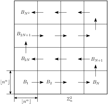
Now, let us start the proof. Let α∈(0,γ)\alpha\in(0,\sqrt{\gamma}) and N=⌈n⌊nα⌋⌉N=\big\lceil\frac{n}{\lfloor n^{\alpha}\rfloor}\big\rceil. We divide the torus ℤn2{\mathbb{Z}}_{n}^{2} into N2N^{2} boxes of size ⌊nα⌋\lfloor n^{\alpha}\rfloor (i.e., each box contains ⌊nα⌋2\lfloor n^{\alpha}\rfloor^{2} sites). The “lower left” box is called B1B_{1} (in this section the torus ℤn2{\mathbb{Z}}_{n}^{2} is identified with [0,n)2⊂ℤ2[0,n)^{2}\subset{\mathbb{Z}}^{2}) and the other boxes are positioned and enumerated following the arrows showed in Figure 4 up to the box BN2B_{N^{2}}. Observe that if nn is not divisible by ⌊nα⌋\lfloor n^{\alpha}\rfloor, then the boxes Bj​NB_{jN}, B(j−1)​N+1B_{(j-1)N+1} on Figure 4 have some area in common for j∈{1,…,N}j\in\{1,\dots,N\}. The same is true for the boxes BjB_{j}, BN2−(j−1)B_{N^{2}-(j-1)} for j∈{1,…,N}j\in\{1,\dots,N\}.

Refer to caption
Figure 4: Enumeration of the boxes BiB_{i}, i∈{1,…,N2}i\in\{1,\dots,N^{2}\}.

Let η∈(0,min⁡{1,12​(γα−1)})\eta\in\big(0,\min\{1,\frac{1}{2}(\frac{\sqrt{\gamma}}{\alpha}-1)\}\big) and for all i∈{1,…,N2}i\in\{1,\dots,N^{2}\}, introduce the following sets

Bi′={x∈ℤn2: there exists ​y∈Bi​ such that ​‖y−x‖∞≤⌊η​nα⌋}.B^{\prime}_{i}=\{x\in{\mathbb{Z}}^{2}_{n}:\text{ there exists }y\in B_{i}\text{ such that }\|y-x\|_{\infty}\leq\lfloor\eta n^{\alpha}\rfloor\}.

Now, consider the torus ℤℓn2{\mathbb{Z}}^{2}_{\ell_{n}} where ℓn=2​⌊η​nα⌋+⌊nα⌋\ell_{n}=2\lfloor\eta n^{\alpha}\rfloor+\lfloor n^{\alpha}\rfloor and fix a box BB of size ⌊nα⌋\lfloor n^{\alpha}\rfloor “centered” in it. Let

B~={x∈ℤℓn2: for all y∈B,∥y−x∥∞≥⌊ηnα⌋}{\tilde{B}}=\{x\in{\mathbb{Z}}^{2}_{\ell_{n}}:\text{ for all }y\in B,\|y-x\|_{\infty}\geq\lfloor\eta n^{\alpha}\rfloor\}

be the “boundary” of the torus ℤℓn2{\mathbb{Z}}^{2}_{\ell_{n}}. For all i∈ℕi\in{\mathbb{N}}, we consider the sequence Y(i)Y^{(i)} (independent of XX) of i.i.d. random elements, where for each i≥1i\geq 1,

Y(i)={Yj,x(i),x∈B~,j≥1},Y^{(i)}=\Big\{Y^{(i)}_{j,x},x\in{\tilde{B}},j\geq 1\Big\},

and the Yj,x(i)Y^{(i)}_{j,x} are independent random variables such that

ℙ[Yj,x(i)=y]=HB(x,y),\mathbb{P}[Y^{(i)}_{j,x}=y]=H_{B}(x,y),

where HB​(x,⋅)H_{B}(x,\cdot) is the entrance law in BB for the simple random walk on the torus ℤℓn2{\mathbb{Z}}^{2}_{\ell_{n}} starting from xx, similarly to (2.1). Using the natural identification of the boxes Bi′B^{\prime}_{i} with ℤℓn2{\mathbb{Z}}^{2}_{\ell_{n}} and the boxes BiB_{i} with BB, each random element Y(i)Y^{(i)} will be viewed as a set of random variables indexed by ∂Bi′\partial B^{\prime}_{i} and j≥1j\geq 1 and taking values in BiB_{i}.

Set V0=0V_{0}=0. For i∈{1,…,N2}i\in\{1,\dots,N^{2}\}, we define inductively (see Figure 5):

σ0(i)\displaystyle\sigma_{0}^{(i)} =Vi−1,\displaystyle=V_{i-1},
τ0(i)\displaystyle\tau_{0}^{(i)} =inf{t≥σ0(i):Xt∈∂Bi′}\displaystyle=\inf\big\{t\geq\sigma_{0}^{(i)}:X_{t}\in\partial B^{\prime}_{i}\big\}

(observe that for i=1i=1 the value of Vi−1=V0V_{i-1}=V_{0} is set to be equal to 00, and, for the next steps, see (3.12) below) and for all j≥1j\geq 1, define

σj(i)\displaystyle\sigma_{j}^{(i)} =inf{t≥τj−1(i):Xt=Yj,Xτj−1(i)(i)},\displaystyle=\inf\Big\{t\geq\tau_{j-1}^{(i)}:X_{t}=Y^{(i)}_{j,X_{\tau^{(i)}_{j-1}}}\Big\},
τj(i)\displaystyle\tau_{j}^{(i)} =inf{t≥σj(i):Xt∈∂Bi′}.\displaystyle=\inf\big\{t\geq\sigma^{(i)}_{j}:X_{t}\in\partial B^{\prime}_{i}\big\}.

Let δ>0\delta>0 and recall that rn=4π​γ​n2​α​ln2​nr_{n}=\frac{4}{\pi}\gamma n^{2\alpha}\ln^{2}n. We also define

Ji=inf{j≥0:∑k=0j(τk(i)−σk(i))≥⌊(1−δ)​rn⌋}J_{i}=\inf\Big\{j\geq 0:\sum_{k=0}^{j}(\tau_{k}^{(i)}-\sigma_{k}^{(i)})\geq\lfloor(1-\delta)r_{n}\rfloor\Big\}

and

βi=σJi(i)+⌊(1−δ)​rn⌋−∑k=0Ji−1(τk(i)−σk(i)).\displaystyle\beta_{i}=\sigma_{J_{i}}^{(i)}+\lfloor(1-\delta)r_{n}\rfloor-\sum_{k=0}^{J_{i}-1}(\tau_{k}^{(i)}-\sigma_{k}^{(i)}).

Finally, we define

Vi=inf{t≥βi:Xt=wi}V_{i}=\inf\big\{t\geq\beta_{i}:X_{t}=w_{i}\big\} (3.12)

where wiw_{i} is the lower left corner point of the box Bi+1B_{i+1}.

Refer to caption
Figure 5: The strategy for covering the box BiB_{i}. We let the walk evolve freely until it hits the boundary of Bi′B^{\prime}_{i}. Then, we force the walk to go rapidly to a random site of ∂Bi\partial B_{i} (this corresponds to the gray parts of the trajectory). This random site is chosen according to the entrance law to BiB_{i} as if we had the torus ℤℓn2{\mathbb{Z}}^{2}_{\ell_{n}} instead of the box Bi′B^{\prime}_{i}. This allows us to dominate the trace of the random walk X^{\hat{X}} on B⊂ℤℓn2B\subset{\mathbb{Z}}^{2}_{\ell_{n}} by the trace of the random walk XX on BiB_{i}.

By transitivity of the simple random walk on the torus ℤn2{\mathbb{Z}}_{n}^{2} we have that

ℙ[𝒯n≤4πγn2ln2n]=ℙx[𝒯n≤4πγn2ln2n]\displaystyle\mathbb{P}\Big[{\mathcal{T}}_{n}\leq\frac{4}{\pi}\gamma n^{2}\ln^{2}n\Big]=\mathbb{P}_{x}\Big[{\mathcal{T}}_{n}\leq\frac{4}{\pi}\gamma n^{2}\ln^{2}n\Big] (3.13)

for all x∈ℤn2x\in{\mathbb{Z}}^{2}_{n}. So, in the rest of the proof we assume that x=0x=0.

Define 𝒮(i)\mathcal{S}^{(i)} as the trace left by the excursions of the random walk XX during the time intervals [σj(i),τj(i)][\sigma^{(i)}_{j},\tau^{(i)}_{j}], 0≤j<Ji0\leq j<J_{i} and [σJi(i),βi][\sigma_{J_{i}}^{(i)},\beta_{i}]. Define the events MiM_{i}, for i∈{1,…,N2}i\in\{1,\dots,N^{2}\} as

Mi\displaystyle M_{i} ={Ji≤ln6n,Bi⊂𝒮(i)}∩{σj+1(i)−τj(i)≤δ4πγn2​αln4⁡n,0≤j<Ji}\displaystyle=\Big\{J_{i}\leq\ln^{6}n,B_{i}\subset\mathcal{S}^{(i)}\Big\}\cap\Big\{\sigma^{(i)}_{j+1}-\tau^{(i)}_{j}\leq\delta\frac{4}{\pi}\gamma\frac{n^{2\alpha}}{\ln^{4}n},0\leq j<J_{i}\Big\}
∩{Vi−βi≤δ4πγn2​αln4⁡n}.\displaystyle\phantom{**}\cap\Big\{V_{i}-\beta_{i}\leq\delta\frac{4}{\pi}\gamma\frac{n^{2\alpha}}{\ln^{4}n}\Big\}.

Observe that ⋂i=1N2Mi\bigcap_{i=1}^{N^{2}}M_{i} is a desired strategy:

{⋂i=1N2Mi}⊂{𝒯n≤4πγn2ln2n}.\displaystyle\Big\{\bigcap_{i=1}^{N^{2}}M_{i}\Big\}\subset\Big\{{\mathcal{T}}_{n}\leq\frac{4}{\pi}\gamma n^{2}\ln^{2}n\Big\}. (3.14)

For i∈{1,…,N2}i\in\{1,\dots,N^{2}\} we introduce the σ\sigma-fields 𝒢Vi=ℱVi∨σ⁡(Y(j),j≤i){\mathcal{G}}_{V_{i}}=\mathcal{F}_{V_{i}}\vee\sigma(Y^{(j)},j\leq i), where ℱVi\mathcal{F}_{V_{i}} is the σ\sigma-field generated the random walk XX until time ViV_{i}. Conditioning iteratively by 𝒢Vi{\mathcal{G}}_{V_{i}} for i∈{1,…,N2}i\in\{1,\dots,N^{2}\} and using the strong Markov property of XX (observe that XX still has the strong Markov property when conditioning by 𝒢Vi{\mathcal{G}}_{V_{i}} since the random elements Y(i)Y^{(i)} are independent of XX), we obtain that

ℙ0​[⋂i=1N2Mi]=(ℙ0​[M1])N2.\mathbb{P}_{0}\Big[\bigcap_{i=1}^{N^{2}}M_{i}\Big]=\big(\mathbb{P}_{0}[M_{1}]\big)^{N^{2}}.

We will now estimate ℙ0​[M1]\mathbb{P}_{0}[M_{1}]. For this, we introduce the σ\sigma-field ℋ{\mathcal{H}} generated by the random element Y(1)Y^{(1)} and by XX within the time intervals ([σj(1),τj(1)],0≤j<J1)([\sigma^{(1)}_{j},\tau^{(1)}_{j}],0\leq j<J_{1}) and [σJ1(1),β1][\sigma_{J_{1}}^{(1)},\beta_{1}]. Define also the events

Φj(1)={σj+1(1)−τj(1)≤δ4πγn2​αln4⁡n}\Phi^{(1)}_{j}=\Big\{\sigma^{(1)}_{j+1}-\tau^{(1)}_{j}\leq\delta\frac{4}{\pi}\gamma\frac{n^{2\alpha}}{\ln^{4}n}\Big\}

for 0≤j<J10\leq j<J_{1} and

ΦJ1(1)={V1−β1≤δ4πγn2​αln4⁡n}.\Phi^{(1)}_{J_{1}}=\Big\{V_{1}-\beta_{1}\leq\delta\frac{4}{\pi}\gamma\frac{n^{2\alpha}}{\ln^{4}n}\Big\}.

By definition of M1M_{1} we have

ℙ0​[M1]\displaystyle\mathbb{P}_{0}[M_{1}] =ℙ0​[J1≤ln6⁡n,B1⊂𝒮(1),⋂j=0J1Φj(1)]\displaystyle=\mathbb{P}_{0}\Big[J_{1}\leq\ln^{6}n,B_{1}\subset\mathcal{S}^{(1)},\bigcap_{j=0}^{J_{1}}\Phi^{(1)}_{j}\Big]
=𝔼0​[𝟏​{J1≤ln6⁡n,B1⊂𝒮(1)}​ℙ0​[⋂j=0J1Φj(1)∣ℋ]].\displaystyle=\mathbb{E}_{0}\Big[{\mathbf{1}}{\{J_{1}\leq\ln^{6}n,B_{1}\subset\mathcal{S}^{(1)}\}}\mathbb{P}_{0}\Big[\bigcap_{j=0}^{J_{1}}\Phi^{(1)}_{j}\mid{\mathcal{H}}\Big]\Big]. (3.15)

Now observe that, conditioned on ℋ{\mathcal{H}}, the events Φj(1)\Phi^{(1)}_{j}, 0≤j≤J10\leq j\leq J_{1}, are independent. Further, in the time interval [τj(1),σj+1(1)][\tau^{(1)}_{j},\sigma^{(1)}_{j+1}], for 0≤j<J10\leq j<J_{1}, we have an excursion of XX starting at point Xτj(1)X_{\tau^{(1)}_{j}} on ∂B1′\partial B^{\prime}_{1} and ending at point Yj,Xτj(1)(1)Y^{(1)}_{j,X_{\tau^{(1)}_{j}}} on ∂B1\partial B_{1}. The last excursion in the time interval [β1,V1][\beta_{1},V_{1}] is conditioned to start from some point in B1′B^{\prime}_{1} and to end at the lower left corner of B2B_{2}. Considering the process S=(St)t≥0S=(S_{t})_{t\geq 0} which under the measure PxP_{x} is a random walk on ℤ2{\mathbb{Z}}^{2} starting at xx, we deduce that

ℙ0​[⋂j=0J1Φj(1)∣ℋ]\displaystyle\mathbb{P}_{0}\Big[\bigcap_{j=0}^{J_{1}}\Phi^{(1)}_{j}\mid{\mathcal{H}}\Big] ≥(infx∈B1′,y∈∂B1ℙx[Xv=y])J1\displaystyle\geq\Big(\inf_{\begin{subarray}{c}x\in B^{\prime}_{1},\\ y\in\partial B_{1}\end{subarray}}\mathbb{P}_{x}[X_{v}=y]\Big)^{J_{1}}
≥(infx∈B1′,y∈∂B1Px[Sv=y])J1\displaystyle\geq\Big(\inf_{\begin{subarray}{c}x\in B^{\prime}_{1},\\ y\in\partial B_{1}\end{subarray}}P_{x}[S_{v}=y]\Big)^{J_{1}}

with v=⌊δ​4π​γ​n2​αln4⁡n⌋v=\big\lfloor\delta\frac{4}{\pi}\gamma\frac{n^{2\alpha}}{\ln^{4}n}\big\rfloor if ⌊δ​4π​γ​n2​αln4⁡n⌋\big\lfloor\delta\frac{4}{\pi}\gamma\frac{n^{2\alpha}}{\ln^{4}n}\big\rfloor and ‖x−y‖1\|x-y\|_{1} have the same parity (where ∥⋅∥1\|\cdot\|_{1} is the 1-norm on ℤn2{\mathbb{Z}}^{2}_{n}) and v=⌊δ​4π​γ​n2​αln4⁡n⌋−1v=\lfloor\delta\frac{4}{\pi}\gamma\frac{n^{2\alpha}}{\ln^{4}n}\rfloor-1 otherwise. Using the local central limit theorem (see e.g. Theorem 2.1.3 in [13]) and the fact that ‖x−y‖1≤4​nα\|x-y\|_{1}\leq 4n^{\alpha} (recall that η<1\eta<1), we obtain

(infx∈B1′,y∈∂B1Px[Sv=y])J1≥exp(−c0​J1​ln4​nδ​γ).\displaystyle\Big(\inf_{\begin{subarray}{c}x\in B^{\prime}_{1},\\ y\in\partial B_{1}\end{subarray}}P_{x}\Big[S_{v}=y\Big]\Big)^{J_{1}}\geq\exp\Big(-\frac{c_{0}J_{1}\ln^{4}n}{\delta\gamma}\Big).

for some constant c0>0c_{0}>0 and nn large enough. From (3.15), we deduce

ℙ0​[M1]≥exp⁡(−c0​ln10​nδ​γ)×ℙ0​[J1≤ln6⁡n,B1⊂𝒮(1)]\displaystyle\mathbb{P}_{0}[M_{1}]\geq\exp\Big(-\frac{c_{0}\ln^{10}n}{\delta\gamma}\Big)\times\mathbb{P}_{0}[J_{1}\leq\ln^{6}n,B_{1}\subset\mathcal{S}^{(1)}] (3.16)

for nn large enough. Let us now bound from below the probability in the right-hand side of (3.16). We start by writing

ℙ0​[J1≤ln6⁡n,B1⊂𝒮(1)]\displaystyle\mathbb{P}_{0}[J_{1}\leq\ln^{6}n,B_{1}\subset\mathcal{S}^{(1)}] ≥ℙ0[J1≤ln6n]−ℙ0[B1⊄𝒮(1)].\displaystyle\geq\mathbb{P}_{0}[J_{1}\leq\ln^{6}n]-\mathbb{P}_{0}[B_{1}\not\subset\mathcal{S}^{(1)}]. (3.17)

Now, let ℚx{\mathbb{Q}}_{x} be the law of a simple random walk X^\hat{X} on ℤℓn2{\mathbb{Z}}^{2}_{\ell_{n}} starting at xx and define the random variables σ^j\hat{\sigma}_{j}, τ^j\hat{\tau}_{j}, β^\hat{\beta}, J^\hat{J} and 𝒮^\hat{\mathcal{S}} for X^\hat{X} analogously to σj(1)\sigma^{(1)}_{j}, τj(1)\tau^{(1)}_{j}, β1\beta_{1} J1J_{1} and 𝒮(1)\mathcal{S}^{(1)} for XX (BB and B~{\tilde{B}} play the role of B1B_{1} and ∂B1′\partial B^{\prime}_{1}, correspondingly). Observe that by construction, the excursions of XX during the time intervals [σj(1),τj(1)][\sigma^{(1)}_{j},\tau^{(1)}_{j}] until time β1\beta_{1} have the same law under ℙ0\mathbb{P}_{0} as the excursions of X^\hat{X} during the time intervals [σ^j,τ^j][\hat{\sigma}_{j},\hat{\tau}_{j}] until time β^\hat{\beta} under ℚx0{\mathbb{Q}}_{x_{0}} where x0:=(⌊η​nα⌋,⌊η​nα⌋)x_{0}:=(\lfloor\eta n^{\alpha}\rfloor,\lfloor\eta n^{\alpha}\rfloor). Therefore, we have

ℙ0​[J1≤ln6⁡n,B1⊂𝒮(1)]\displaystyle\mathbb{P}_{0}[J_{1}\leq\ln^{6}n,B_{1}\subset\mathcal{S}^{(1)}] ≥ℚx0[J^≤ln6n]−ℚx0[B⊄𝒮^]\displaystyle\geq{\mathbb{Q}}_{x_{0}}[\hat{J}\leq\ln^{6}n]-{\mathbb{Q}}_{x_{0}}[B\not\subset\hat{\mathcal{S}}]
≥ℚx0[J^≤ln6n]−ℚx0[𝒯ℓn>(1−δ)rn].\displaystyle\geq{\mathbb{Q}}_{x_{0}}[\hat{J}\leq\ln^{6}n]-{\mathbb{Q}}_{x_{0}}[{\mathcal{T}}_{\ell_{n}}>(1-\delta)r_{n}]. (3.18)

Using the fact that η<12​(γα−1)\eta<\frac{1}{2}(\frac{\sqrt{\gamma}}{\alpha}-1) we can choose δ>0\delta>0 such that δ<1−α2​(1+2​η)2γ\delta<1-\frac{\alpha^{2}(1+2\eta)^{2}}{\gamma}, then by (1.3) we obtain

ℚx0[𝒯ℓn>(1−δ)rn]≤14{\mathbb{Q}}_{x_{0}}[{\mathcal{T}}_{\ell_{n}}>(1-\delta)r_{n}]\leq\frac{1}{4} (3.19)

for all nn large enough.

Now let us show that ℚx0[J^≤ln6n]≥12{\mathbb{Q}}_{x_{0}}[\hat{J}\leq\ln^{6}n]\geq\frac{1}{2} for all large enough nn. We first introduce the following event

Λ={there exists j∈{0,…,J^−1} such that τ^j−σ^j≤rnln6⁡n}.\Lambda=\Big\{\text{there exists $j\in\{0,\dots,\hat{J}-1\}$ such that $\hat{\tau}_{j}-\hat{\sigma}_{j}\leq\frac{r_{n}}{\ln^{6}n}$}\Big\}.

Since J^≤rn⌊η​nα⌋\hat{J}\leq\frac{r_{n}}{\lfloor\eta n^{\alpha}\rfloor} (indeed, as any excursion starts from ∂B\partial B and ends at B~\tilde{B}, we need at least ⌊η​nα⌋\lfloor\eta n^{\alpha}\rfloor steps to complete it), we obtain by the Markov property

ℚx0[J^>ln6n]\displaystyle{\mathbb{Q}}_{x_{0}}[\hat{J}>\ln^{6}n] ≤ℚx0​[Λ]\displaystyle\leq{\mathbb{Q}}_{x_{0}}[\Lambda]
≤∑j=0⌊rn​⌊η​nα⌋−1⌋−1ℚx0[τ^j−σ^j≤rnln6⁡n]\displaystyle\leq\sum_{j=0}^{\lfloor r_{n}\lfloor\eta n^{\alpha}\rfloor^{-1}\rfloor-1}{\mathbb{Q}}_{x_{0}}\Big[\hat{\tau}_{j}-\hat{\sigma}_{j}\leq\frac{r_{n}}{\ln^{6}n}\Big]
≤rn⌊η​nα⌋supx∈∂Bℚx[maxt≤rn​ln−6​n∥X^t∥1≥ηnα]\displaystyle\leq\frac{r_{n}}{\lfloor\eta n^{\alpha}\rfloor}\sup_{x\in\partial B}{\mathbb{Q}}_{x}\Big[\max_{t\leq r_{n}\ln^{-6}n}\|\hat{X}_{t}\|_{1}\geq\eta n^{\alpha}\Big]
=rn⌊η​nα⌋supx∈∂BPx[maxt≤rn​ln−6​n∥St∥1≥ηnα].\displaystyle=\frac{r_{n}}{\lfloor\eta n^{\alpha}\rfloor}\sup_{x\in\partial B}P_{x}\Big[\max_{t\leq r_{n}\ln^{-6}n}\|S_{t}\|_{1}\geq\eta n^{\alpha}\Big]. (3.20)

Using item b) of Proposition 2.1.2 in [13], we obtain that there exist positive constants c1c_{1} and c2c_{2} such that

supx∈∂BPx[maxt≤rn​ln−6​n∥S(t)∥1≥ηnα]≤c1exp(−c2η2γ−1ln4n).\sup_{x\in\partial B}P_{x}\Big[\max_{t\leq r_{n}\ln^{-6}n}\|S(t)\|_{1}\geq\eta n^{\alpha}\Big]\leq c_{1}\exp(-c_{2}\eta^{2}\gamma^{-1}\ln^{4}n).

Together with (3.20) this implies that ℚx0[J^>ln6n]→0{\mathbb{Q}}_{x_{0}}[\hat{J}>\ln^{6}n]\to 0 as n→∞n\to\infty and therefore ℚx0[J^≤ln6n]≥12{\mathbb{Q}}_{x_{0}}[\hat{J}\leq\ln^{6}n]\geq\frac{1}{2} for nn large enough. Combining this fact with (3.17), (3.18), and (3.19) we obtain that

ℙ0​[J1≤ln6⁡n,B1⊂𝒮(1)]≥14\mathbb{P}_{0}[J_{1}\leq\ln^{6}n,B_{1}\subset\mathcal{S}^{(1)}]\geq\frac{1}{4} (3.21)

for all nn large enough. Finally, using (3.16), (3.14) and (3.13) we deduce that

ℙ[𝒯n≤4πγn2ln2n]\displaystyle\mathbb{P}\Big[{\mathcal{T}}_{n}\leq\frac{4}{\pi}\gamma n^{2}\ln^{2}n\Big] ≥(14​exp⁡(−c0​ln10​nδ​γ))N2\displaystyle\geq\Big(\frac{1}{4}\exp\Big(-\frac{c_{0}\ln^{10}n}{\delta\gamma}\Big)\Big)^{N^{2}}
≥exp⁡(−2​n2​(1−α)​(c0δ​γ​ln10​n+2​ln⁡2))\displaystyle\geq\exp\Big(-2n^{2(1-\alpha)}\Big(\frac{c_{0}}{\delta\gamma}\ln^{10}n+2\ln 2\Big)\Big)

for nn large enough. Since α∈(0,γ)\alpha\in(0,\sqrt{\gamma}) can be chosen arbitrarily close to γ\sqrt{\gamma} we obtain the lower bound in Theorem 1.1. ∎

Acknowledgments

The authors thank the French-Brazilian program Chaires Françaises dans l’État de São Paulo which supported the visit of F.C. to Brazil. S.P. and M.V. were partially supported by CNPq (grants 300886/2008–0 and 301455/2009–0). The last three authors thank FAPESP (2009/52379–8) for financial support. F.C. is partially supported by CNRS, UMR 7599 LPMA.

References

  • [1] D. Aldous, J. Fill (2010) Reversible Markov Chains and Random Walks on Graphs. In preparation. http://www.stat.berkeley.edu/˜aldous/RWG/book.html
  • [2] D. Belius (2013) Gumbel fluctuations for cover times in the discrete torus. To appear in: Probab. Theory Relat. Fields
  • [3] I. Benjamini, O. Gurel-Gurevich, B. Morris (2013) Linear cover time is exponentially unlikely Probab. Theory Relat. Fields 155 (1-2), 451–461.
  • [4] M. Bramson, O. Zeitouni (2009) Tightness for a family of recursion equations. Ann. Probab. 37 (2), 615–653.
  • [5] A. Dembo (2005) Favorite points, cover times and fractals. In: Lectures on probability theory and statistics (St Flour 2003). Lecture Notes in Math., 1869, 1–101, Springer, Berlin.
  • [6] A. Dembo, Y. Peres, J. Rosen, O. Zeitouni (2004) Cover times for Brownian motion and random walks in two dimensions. Ann. Math. (2) 160 (2), 433–464.
  • [7] A. Dembo, Y. Peres, J. Rosen, O. Zeitouni (2006) Late points for random walks in two dimensions. Ann. Probab. 34 (1), 219–263.
  • [8] J. Ding (2012) On cover times for 2D lattices. Electr. J. Probab. 17 (45), 1–18.
  • [9] U. Einmahl (1989) Extensions of results of Komlós, Major, and Tusnády to the multivariate case. J. Multivariate Anal. 28 (1), 20–68.
  • [10] J. Goodman, F. den Hollander (2012) Extremal geometry of a Brownian porous medium. To appear in: Probab. Theory Relat. Fields
  • [11] J. Kahn, J. Kim, L. Lovàsz, V. Vu (2000) The cover time, the blanket time, and the Matthews bound. 41st Annual Symp. Found. Computer Science (Redondo Beach, CA, 2000), 467–475, IEEE Comput. Soc. Press, Los Alamitos, CA.
  • [12] J. Komlós, P. Major, G. Tusnády (1975) An approximation of partial sums of independent RV’s and the sample DF. I. Z. Wahrsch. Verw. Gebiete 32, 111–131.
  • [13] G. Lawler, V. Limic (2010) Random walk: a modern introduction. Cambridge Studies in Advanced Mathematics, 123. Cambridge University Press, Cambridge,
  • [14] P. Matthews (1988) Covering problems for Markov chains. Ann. Probab. 16 (3), 1215–1228.
  • [15] S. Popov, A. Teixeira (2013) Soft local times and decoupling of random interlacements. To appear in: J. European Math. Soc.
  • [16] Z. Shi (2006) Problèmes de recouvrement et points exceptionnels pour la marche aléatoire et le mouvement Brownien. (Séminaire Bourbaki.) Astérisque 307, 469–480.
  • [17] H. Wilf (1989) The editor’s corner: the white screen problem. Amer. Math. Monthly 96 (8), 704–707.