A non-linear rod model for folded elastic strips

We consider an inextensible elastic plate of thickness $h$ and width $w$ with a large aspect-ratio, $h\ll w$. In its undeformed configuration, the strip is planar. Under the action of a mechanical load, it is deformed into a 3d shape, as sketched in figure 2.

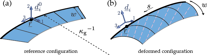
The deformed strip is parameterized by a space curve $\underline{r}(s)$, called the centerline, and by an orthonormal frame $(\underline{d}_{1}(s),\underline{d}_{2}(s),\underline{d}_{3}(s))$, called the material frame. To define the centerline, we pick one of the lateral edges, which is the thick curve in the figure 2. The name ‘centerline’ is used for consistency with the theory of rods even though this curve is off the center of the strip. We denote by $s$ be the arc-length along this edge, and by $\underline{r}(s)$ the position in space of the centerline. The derivation with respect to arc-length is denoted by a prime. By definition, the tangent $\underline{r}^{\prime}(s)$ is a unit vector. Since the plate is inextensible, the arc-length $s$ will be used as a Lagrangian variable. The direct orthonormal frame $\underline{d}_{i}(s)$, with $i=1,2,3$, is defined in such a way that $\underline{d}_{3}$ is the tangent to the centerline,

and that $\underline{d}_{1}(s)$ and $\underline{d}_{3}(s)$ span the tangent plane to the midsurface of the elastic strip at the point $\underline{r}(s)$. Then, the unit vector $\underline{d}_{2}(s)=\underline{d}_{3}(s)\times\underline{d}_{1}(s)$ is normal to the midsurface at the edge $\underline{r}(s)$. By construction, the material frame is orthonormal and direct:

for any indices $i,j=\{1,2,3\}$ and for any $s$. Here, $\delta_{ij}$ denotes Kronecker’s symbol, equal to $1$ if $i=j$ and $0$ otherwise.

The rate of rotation of the material frame with respect to the arc-length is captured by a vector $\underline{\omega}(s)$, which we call the Darboux vector or the twist-curvature strain. It is such that, for any $i=1,2,3$,

In classical rod theories, the rotation gradient $\underline{\omega}(s)$ measures the strain associated with the bending and twisting modes. Here, we use a plate model, and the bending strain is measured by the curvature form (second fundamental form) of the mid-surface, which we denote by $\underline{\underline{k}}$. Near a generic point $\underline{r}(s)$ on the centerline, we use the frame $(\underline{d}_{3}(s),\underline{d}_{1}(s))$ tangent to surface: in this frame, the curvature tensor $\underline{\underline{k}}(s)$ is represented by a symmetric matrix,

From the differential geometry of surfaces [13, 14], the gradient of the unit normal to a surface along any tangent direction can be computed from the second fundamental form. In particular, if we consider the gradient of the normal $\underline{d}_{2}(s)$ along the tangent $\underline{d}_{3}(s)$ to the centerline, we have $\underline{d}_{2}^{\prime}(s)=-\underline{\underline{k}}(s)\cdot\underline{d}_{3}(s)=-(k_{13}(s)\,\underline{d}_{1}(s)+k_{33}(s)\,\underline{d}_{3}(s))$. Identifying with the case $i=2$ equation (3), we find that the plate’s bending strain and the equivalent rod’s curvature strain are related by: $k_{13}(s)=\omega_{3}(s)$ and $k_{33}(s)=-\omega_{1}(s)$, where $\omega_{j}=\underline{\omega}\cdot\underline{d}_{j}$ denote the components of the Darboux vector in the material frame. We use this to express the second fundamental form of the midsurface of the plate, in terms of the Darboux vector $\underline{\omega}$ of the equivalent rod:

We assume that the midsurface of the plate is inextensible. This has two consequences. First, by Gauss’ theorema egregium [13], its Gauss curvature, defined as the determinant of $\underline{\underline{k}}$, is zero:

Second, we note that the quantity $\omega_{2}$, which defines the geodesic curvature of the centerline with respect to the midsurface, is conserved by isometries [13]. Let $\kappa_{\mathrm{g}}=\omega_{2}^{0}$ denote the signed curvature of the edge (centerline) in the flat configuration of reference: in the actual configuration, the conservation of the geodesic curvature implies

In equation (4), we have expressed the ‘microscopic’ strain $\underline{\underline{k}}$ in terms of the strain $\underline{\omega}$ of the equivalent rod, and of an additional ‘internal’ strain variable $k_{11}$. Equation (5) is a kinematic constraint. It could be used to eliminate the strain variable $k_{11}$ in favor of $\underline{\omega}$; we will refrain to do so, however, as this requires the additional assumption $\omega_{1}\neq 0$. Equation (6) is a second kinematic constraint applicable to the equivalent rod model.

Let us denote by $k^{*}$ the typical curvature of the plate, $|\underline{\underline{k}}|\sim k^{*}$. We assume that the strip is narrow, in the sense that the variations of the curvature tensor on distances comparable to the width $w$ remain small compared to $k^{*}$: $w\,|\underline{\nabla}\underline{\underline{k}}|\ll k^{*}$. Therefore, we ignore the dependence of the curvature strain on the transverse coordinate: in the entire cross-section containing the centerline point $\underline{r}(s)$, we approximate the curvature tensor by $\underline{\underline{k}}(s)$. This approximation has been used in the past to describe plates with straight centerlines [30]. It is possible to go beyond this approximation [31], as required when the curvature becomes large at localized spots along one of the edges [33] — we will refer to this model as a strip of finite width. An even more general model, applicable to strips of finite width and non-zero geodesic curvature, has been recently derived in [12].

We return to our small width approximation: the bending energy of the inextensible plate $E_{\mathrm{p}}$ can be integrated along the transverse direction, which yields

where $D=E\,h^{3}/(12(1-\nu^{2})))$ is the bending modulus of the plate, $E$ its Young’s modulus, $\nu$ its Poisson’s ratio and $h$ its thickness. For a $2\times 2$ matrix, the following identity holds: $\tr^{2}\underline{\underline{k}}=\tr\left(\underline{\underline{k}}^{2}\right)+2\,\det\underline{\underline{k}}$. Dropping the determinant using the inextensibility condition (5), one can rewrite the elastic energy as

where $B=w\,D$ is a rod-type bending modulus, and the double contraction operator is defined by $\underline{\underline{a}}:\underline{\underline{b}}=\tr(\underline{\underline{a}}\cdot\underline{\underline{b}})=\sum_{ij}a_{ij}\,b_{ji}$. Note that when $k_{11}$ is eliminated using the constraint (5), the elastic energy $E_{\mathrm{p}}$ coincides with that derived by Sadowsky [30]:

We derive the equivalent rod model for our thin strip simply by viewing the energy $E_{\mathrm{p}}$ in equation (8) as the energy of a thin rod. The equivalent thin rod has one internal degree of freedom $k_{11}$ and is subjected to two kinematical constraints $\mathcal{C}_{\mathrm{d}}(\omega_{1},\omega_{3},k_{11})$ and $\mathcal{C}_{\mathrm{g}}(\omega_{2})$. In the A, we derive the equations for a rod of this type. The condition of equilibrium of the internal variable reads

Here, $\delta E_{\mathrm{p}}/\delta\omega_{i}$ and $\delta E_{\mathrm{p}}/\delta k_{11}$ denote the functional derivative of the elastic energy $E_{\mathrm{p}}$ with respect to the local strain $\omega_{i}(s)$ and internal variable $k_{11}(s)$, respectively. These equations were obtained by extending equations (87a–87b) of the appendix to the case of two constraints, and by identifying the internal degree of freedom $k=k_{11}$ and the energy $E_{\mathrm{el}}=E_{\mathrm{p}}$. The two Lagrange multipliers $\lambda_{\mathrm{d}}$ and $\lambda_{\mathrm{g}}$ are associated with the two constraint. For convenience, they have been rescaled with the bending modulus $B$, i.e. the quantity $\lambda$ in the appendix is replaced with $B\,\lambda_{\mathrm{d}}$ and $B\,\lambda_{\mathrm{g}}$.

Equation (9a) can be interpreted as the cancellation of the total generalized force acting on the internal variable, which is the sum of the standard force in the first term, and of constraint forces [34] in the last two terms. Similarly, the constitutive law in equation (9b) is made up of the usual contribution in rod theory, whereby the internal moment is the gradient of the elastic energy with respect to the twist and curvature strains, plus two other terms which are known as (generalized) constraint forces.

Using the explicit form of the energy $E_{\mathrm{p}}$ and of the constraints $\mathcal{C}_{\mathrm{d}}$ and $\mathcal{C}_{\mathrm{g}}$, equation (9a) yields

This equation will be used to eliminate the internal variable $k_{11}$ whenever it appears. In particular, the developability constraint in equation (5) takes the form

The second equation (9b) yields

Eliminating $k_{11}$ and projecting onto the material basis, we find the expressions of the twisting and bending moments $m_{i}=\underline{m}\cdot\underline{d}_{i}$:

This is the constitutive law for a narrow elastic developable strip in the language of rods.

The expression of the constraints in equations (6) and (11) and the constitutive law (12) are the main results of of section 2. They translate the inextensible strip model into the language of Kirchhoff’s rods. Even though the strip is linearly elastic, its constitutive law is effectively non-linear because of the developability constraint.

We emphasize that the cross-sections of the strip are allowed to bend, as sketched in figure 2(b): this is required to preserve developabitility when the centerline is both twisted and bent, i.e. when both $\omega_{1}$ and $\omega_{3}$ are non-zero. We found that the strip is equivalent to an Euler-Bernoulli rod — for classical rods, the latter model is usually justified by assuming that the cross-sections do not bend but this is just a coincidence.

The strong formulation of the equilibrium of elastic rods is known as the Kirchhoff equations [22]. It can be derived by integration by parts from the principle of virtual work, as explained in A:

Here, $\underline{n}$ is the Lagrange multiplier associated with the inextensibility and Euler-Bernoulli constraints, which can be interpreted as the internal force. Given a distribution of external force $\underline{p}(s)$ and moment $\underline{q}(s)$, one can find the equilibria of the strip by solving the kinematical equations (1–3), the contraints (6) and (11), the constitutive law (12) and the equilibrium (13) for the unknowns $\underline{r}(s)$, $\underline{d}_{i}(s)$, $\omega_{i}(s)$, $\lambda_{\mathrm{d}}(s)$ and $\lambda_{\mathrm{g}}(s)$.

The planar configuration of the bistrip is show in figure 3: in this configuration, the curvature of the central fold coincides with the geodesic curvature $\kappa_{\mathrm{g}}$.

The outer and inner flaps, on each side of the central fold, are labelled by $(+)$ and $(-)$, respectively.

A typical 3d configuration of the bistrip is shown in figure 4.

To apply the analysis of section 2 to each of these flaps, we attach a material frame $\underline{d}_{i}^{(\epsilon)}$, with $i=1,2,3$ and $\epsilon=\pm$ to them. Let us denote by $\underline{R}(s)$ the common ridge, and $s$ the arc-length along this ridge. We use this ridge as the centerline for both flaps: in the notations of the previous section, $\underline{r}^{(+)}(s)=\underline{r}^{(-)}(s)=\underline{R}(s)$.

We observe that the tangent material vectors $\underline{d}_{3}^{(\pm)}$ to both flaps are identical, since they share the same centerline: by equation (1), $\underline{d}_{3}^{(+)}(s)={\underline{r}^{(+)}}^{\prime}(s)=\underline{R}^{\prime}(s)={\underline{r}^{(-)}}^{\prime}(s)=\underline{d}_{3}^{(-)}(s)$. This allows us to define the bisecting frame $\underline{D}_{\mu}(s)$, with $\mu=I,I\!\!I,I\!\!I\!\!I$ as follows. Let us first define $\underline{D}_{I\!\!I\!\!I}(s)$ to be the unit tangent to the ridge,

which coincides with the other tangents, $\underline{D}_{I\!\!I\!\!I}(s)=\underline{d}_{3}^{(+)}(s)=\underline{d}_{3}^{(-)}(s)$. The vector $\underline{D}_{I}(s)$ is defined as the unit vector that bisects the directions spanned by $\underline{d}_{1}^{(+)}(s)$ and $\underline{d}_{1}^{(-)}(s)$, as shown in the insets of figure 4. Similarly, the vector $\underline{D}_{I\!\!I}(s)$ is the unit vector that bisects the directions spanned by $\underline{d}_{2}^{(+)}(s)$ and $\underline{d}_{2}^{(-)}(s)$. By construction, the bisecting frame is an orthonormal frame,

for any pair of indices, $\mu,\nu=I,I\!\!I,I\!\!I\!\!I$. As a result, the gradient of rotation of the bisecting frame $\underline{D}_{\mu}$ can be measured by a Darboux vector $\underline{\Omega}$ such that

The star symbols in equation labels, as in equations (14) and (16), will be used to mark any equation that defines the equivalent rod model.

Let us denote by $\beta$ half of the bending angle of the ridge, see the inset of figure 4(a). This angle can be defined as a signed quantity if we use the orientation provided by the tangent $\underline{D}_{I\!\!I\!\!I}=\underline{R}^{\prime}$: by convention $\beta$ is positive in the figure. In terms of the parameter $\beta$, the dihedral angle at the ridge writes $\pi-2\,\beta$.

The local material frames $\underline{d}_{i}^{(\epsilon)}$ ($i=1,2,3$ and $\epsilon=\pm$) can be reconstructed in terms of the bisecting frame and of the angle $\beta$ as follows:

By this equation, the entire bistrip can be reconstructed in terms of $\underline{R}$, $\underline{D}_{\mu}$ and $\beta$. Therefore, we use the ridge $\underline{R}$, the bisecting frame $\underline{D}_{\mu}$ and the ridge angle $\beta$ as the main unknowns. We shall show that the bistrip is equivalent to a rod having a centerline $\underline{R}(s)$ and a material frame $\underline{D}_{\mu}(s)$. The kinematic equations (14) shows that this equivalent rod is effectively an inextensible, Navier-Bernoulli rod — we emphasize that the cross-sections are not assumed to be rigid, however, as already discussed in section 2. The rest of this section is concerned about deriving the constitutive law for the equivalent rod that captures the elasticity of the flaps and of the ridge.

By differentiating equation (17) with respect to arc-length $s$, and identifying the result with equation (3) defining the local strains $\underline{\omega}^{(\epsilon)}$ in each flap, $\epsilon=\pm$, we obtain the following expression of the local strains:

Note that the second term is associated with the ‘internal’ degree of freedom $\beta$ associated with the ridge angle.

To use the constitutive laws for a single strip derived earlier, we shall need the components of $\underline{\omega}^{(\epsilon)}$ in the local material frame, which we denote by $\omega^{(\epsilon)}_{i}=\underline{\omega}^{(\epsilon)}\cdot\underline{d}_{i}^{(\epsilon)}$ in the local frames. Projecting the previous equation, we find

In the right-hand side, we denote by $\Omega_{\mu}=\underline{\Omega}\cdot\underline{D}_{\mu}$ the projections of the strain vector $\underline{\Omega}$ of the equivalent rod in its own material (bisecting) frame $\underline{D}_{\mu}$, with $\mu=I,I\!\!I,I\!\!I\!\!I$.

Let us denote by $\underline{p}(s)$ and $\underline{q}(s)$ the force and moment applied across the ridge, per unit arc-length $\mathrm{d}s$, by the inner region $(-)$ onto the outer region $(+)$. The outer flap feels a force $\underline{p}^{(+)}(s)=+\underline{p}(s)$ and moment $\underline{q}^{(+)}(s)=+\underline{q}(s)$. By the principle of action-reaction, the inner flap feels the opposite force and moment, $\underline{p}^{(-)}(s)=-\underline{p}(s)$ and moment $\underline{q}^{(-)}(s)=-\underline{q}(s)$. We write this in compact form as

for $\epsilon=\pm$.

We model the central fold as an elastic hinge. The twisting moment $\underline{q}(s)\cdot\underline{R}^{\prime}(s)$ is therefore assumed to be a function of the angle $\beta$:

where $Q_{\mathrm{r}}$ is the constitutive law of the ridge. By convention, the argument of $Q_{\mathrm{r}}$ is the turning angle $2\,\beta$ at the ridge, and not $\beta$. This is motivated by the fact that the work done by the ridge is $(2\,\delta\beta)\,Q_{\mathrm{r}}(2\,\beta)$ when the parameter $\beta$ is incremented by $\delta\beta$.

Assuming that the constitutive law of the ridge is linear, we write

where $K_{\mathrm{r}}$ is the stiffness of the ridge, and $\beta_{\textrm{n}}$ the natural value of the angle $\beta$. By creasing the strip, one induces irreversible deformations at the ridge: this is modeled by changing the value of $\beta_{\mathrm{n}}$.

Equation (13a) expresses the balance of force in each flap. With our current notations, it can be rewritten as ${\underline{n}^{(\epsilon)}}^{\prime}(s)+\underline{p}^{(\epsilon)}(s)=\underline{0}$, where $\epsilon=\pm$ labels the flaps and $\underline{n}^{(\epsilon)}$ denotes the internal force in each flap. We define the total internal force $\underline{N}(s)$ in the bistrip,

By summing the local balance of forces and using the definition of $\underline{p}^{(\epsilon)}$ in equation (20), we find that the bistrip satisfies the global balance of forces

External force applied on the bistrip could be considered by adding a term in the left-hand side, as in the classical theory of rods.

Let us now turn to the balance of moments, which can be written in each flap as in equation (13b). Recalling that the two flaps share the same tangent $\underline{r}^{\prime}=\underline{R}^{\prime}=\underline{D}_{I\!\!I\!\!I}$, we have ${\underline{m}^{(\epsilon)}}^{\prime}+\underline{D}_{I\!\!I\!\!I}\times\underline{n}^{(\epsilon)}+\underline{q}^{(\epsilon)}=\underline{0}$. In terms of the total moment $\underline{M}(s)$ in the bistrip, defined by

we write the global balance of moment in the bistrip as

In equations (25) and (27), we have recovered the classical Kirchhoff equation for the equilibrium of thin rods: these equations express the global balance of forces and moments in the bistrip.

The global balance of moments (27) does not involve the internal twisting moment due to the ridge, $Q_{\mathrm{r}}$. A second equation for the balance of moments can be derived by projecting the local balance of moments in each strip onto the shared tangent: ${\underline{m}^{(\epsilon)}}^{\prime}\cdot\underline{R}^{\prime}+\underline{q}^{(\epsilon)}\cdot\underline{R}^{\prime}=0$. Subtracting the equations corresponding to $\epsilon=+$ and $\epsilon=-$, and expressing $\underline{q}^{(\pm)}$ in terms of $Q_{\mathrm{r}}$ using equations (21) and (22), we have

where $\underline{\Delta}$ is half the difference of the internal moments:

As suggested by the presence of the ridge moment $Q_{\mathrm{r}}$, equation (28) expresses the balance of moments at the ridge. It can be viewed as the equation that sets the internal degree of freedom $\beta$.

Two kinematic constraints are applicable in each flap $\epsilon=\pm$: the geodesic constraint $\mathcal{C}_{\mathrm{g}}^{(\epsilon)}=0$ and the developability constraint $\mathcal{C}_{\mathrm{d}}^{(\epsilon)}=0$, see equations (5) and (6). Below, we express these constraints in terms of the centerline $\underline{R}$, of the bisecting frame $\underline{D}_{\mu}$, and of the ridge angle $\beta$. This yields effective kinematic constraints that are applicable to the equivalent rod.

Let us start by the geodesic constraint in equation (6). The geodesic curvature $\kappa_{\mathrm{g}}$ has been interpreted in figure 3, and is identical in both flaps: $\omega_{2}^{(+)}(s)=\omega_{2}^{(-)}(s)=\kappa_{\mathrm{g}}$. In particular, the average of the local curvature reads $\frac{1}{2}\,\left(\omega_{2}^{(-)}(s)+\omega_{2}^{(+)}(s)\right)=\kappa_{\mathrm{g}}$. Using equation (19b), we can rewrite the left-hand side in terms of the strain $\underline{\Omega}$ of the equivalent rod:

By this kinematic constraint, the internal degree of freedom $\beta$ appears to be a function of the curvature strain $\Omega_{I\!\!I}$. We could eliminate $\beta$ in favor of $\Omega_{I\!\!I}$ using this equation. We shall instead view $\beta$ and $\Omega_{I\!\!I}$ as two degrees of freedom subjected to the constraint (30): this makes the final equations easier to interpret.

A second constraint follows from the equality $\omega_{2}^{(+)}(s)=\omega_{2}^{(-)}(s)$: when expressed in terms of $\underline{\Omega}$ as above, it reads $\Omega_{I}\,\sin\beta=0$. We shall ignore the special case $\beta=0$: as explained in section 4.2, the bistrip is then on the boundary of the space of configurations and the equations of equilibrium are inapplicable anyway. Under the assumption $\beta\neq 0$, we have:

In view of the two constraints just derived, we can simplify the expressions of the local strains given earlier in equations (19a) and (19c):

The developability constraint in equation (11) can be simplified as well:

where we have introduced an auxiliary variable $\sigma(s)=\epsilon\,\omega_{1}^{(\epsilon)}(s)$ which is given in terms of $\underline{\Omega}$ by

We note that the first term in equation (28) expressing the balance of moments at the ridge can be written in coordinates as: $\underline{\Delta}^{\prime}\cdot\underline{D}_{I\!\!I\!\!I}=(\underline{\Delta}\cdot\underline{D}_{I\!\!I\!\!I})^{\prime}-\Delta\cdot\underline{D}_{I\!\!I\!\!I}^{\prime}={\Delta_{I\!\!I\!\!I}}^{\prime}-\underline{\Delta}\cdot(\underline{\Omega}\times\underline{D}_{I\!\!I\!\!I})$, where $\underline{\Omega}\times\underline{D}_{I\!\!I\!\!I}=\Omega_{I\!\!I}\,\underline{D}_{I}$ by the constraint in equation (31). Here, we denote by $\Delta_{\mu}=\underline{\Delta}\cdot\underline{D}_{\mu}$ and $\Omega_{\mu}=\underline{\Omega}\cdot\underline{D}_{\mu}$ the components of the differential internal moment $\underline{\Delta}$ and of the twist-curvature strain $\underline{\Omega}$ in the bisecting frame. We can therefore rewrite the equilibrium of the ridge as

To obtain a complete set of equations for the bistrip, we need the expressions of the total internal moment $\underline{M}$ and of the differential internal moment $\underline{\Delta}$ appearing in the equations of equilibrium. We derive the constitutive laws of the bistrip below, by combining the local constitutive law in each flap, and expressing them in terms of the twist-curvature strain $\underline{\Omega}$ of the effective rod.

Let us denote the average over the two flaps $\epsilon=\pm$ by angular brackets: $\langle f^{(\epsilon)}\rangle_{\epsilon}=\frac{1}{2}(f_{-}+f_{+})$. In terms of the Lagrange multipliers $\lambda_{\mathrm{d}}^{(\epsilon)}$ associated with the developability constraint in each flap, we define the following quantities:

Inserting the expression for $\lambda_{\mathrm{d}}^{(\epsilon)}$ found in equation (33), we find explicit expressions for the auxiliary variables $b_{k}^{\pm}$:

The Lagrange multipliers $\lambda_{\mathrm{g}}^{(\epsilon)}$ associated with the geodesic constraints are eliminated in favor of their average $\Lambda_{+}(s)=\langle\lambda_{\mathrm{g}}^{(\epsilon)}(s)\rangle_{\epsilon}$ and half-difference $\Lambda_{-}(s)=\langle\epsilon\,\lambda_{\mathrm{g}}^{(\epsilon)}(s)\rangle_{\epsilon}$: for $\epsilon=\pm$, they can be reconstructed by

We view $\Lambda_{+}(s)$ and $\Lambda_{-}(s)$ as quantities attached to the equivalent rod: they are the Lagrange multipliers associated to the two kinematic constraints (30) and (31).

Let us now consider the local constitutive law in equation (12), which provides the expression of the internal moment $\underline{m}^{(\epsilon)}$ in each flap as a function of $\lambda_{\mathrm{d}}^{(\epsilon)}$, $\lambda_{\mathrm{g}}^{(\epsilon)}$ and $\omega_{2}^{(\epsilon)}$. These quantities can be expressed in terms of the properties of the equivalent rod, using equations (36), (38) and (6), respectively. This yields

Inserting the expressions of the local strains $\omega_{1}^{(\epsilon)}$ and $\omega_{3}^{(\epsilon)}$ and of the local frame $\underline{d}_{i}^{(\epsilon)}$ in equations (32) and (17), we obtain the following expressions of the internal moments $\underline{M}$ and $\underline{\Delta}$ defined in equations (26) as (29):

This equation is the main result of section 3, and one of the main results of our paper. It yields the constitutive law of the rod that is equivalent to the bistrip, and captures the details of how the strip deforms at the ‘microscopic’ scale $w$. The constitutive law is geometrically exact and handles large deformations of the cross-section: the inextensibility of the strip is treated exactly, the cross-sections of the flaps may bend significantly, and the angle $\beta$ can change by a finite amount. The constitutive law is non-linear because of the geometry: the coefficients $b_{i}^{\pm}(\beta,\beta^{\prime},\Omega_{I\!\!I},\Omega_{I\!\!I\!\!I})$ in the matrix above depend non-linearly on the strains through equations (37). By contrast, the underlying plate model makes use of a linear constitutive law: the bending energy of the plate is quadratic with respect to the strain, see equation (7).

This constitutive law (39) depends on the bending strain $\Omega_{I\!\!I}$ — recall that the other bending mode $\Omega_{I}$ is frozen by equation (31) — and on the twisting strain $\Omega_{I\!\!I\!\!I}$, like in the classical theory of thin elastic rods. It also depends on the internal degree of freedom $\beta$ and on its derivative $\beta^{\prime}$, and on the Lagrange multipliers $\Lambda_{+}$ and $\Lambda_{-}$ associated with the two applicable constraints.

The expression of $\Delta_{I\!\!I}$ has been omitted in the constitutive law (39), as it does not appear in the equations of equilibrium: it is absent from equation (35) expressing the balance of moments at the ridge. For reference, its expression is $\Delta_{I\!\!I}(s)=\sin^{2}\beta(s)\,b_{1}^{-}\big(\beta(s),\Omega_{I\!\!I}(s),\Omega_{I\!\!I\!\!I}(s),\beta^{\prime}(s)\big)\,\Omega_{I\!\!I}(s)+\cos\beta(s)\,\Lambda_{-}(s)$.

We recapitulate the equations that govern the bistrip, collecting them by family: these are all the equations that we have marked by a star symbol so far.

• •

  The main unknowns of the model are (i) the centerline $\underline{R}(s)$ and a direct orthonormal frame $\big(\underline{D}_{\mu}(s)\big)_{\mu=1,2,3}$, as usual in rod theory; and (ii) an ‘internal’ degree of freedom, namely the ridge angle $\beta(s)$.

• •

  The kinematic equation defining the strain $\underline{\Omega}$ reads

  $$\underline{D}_{\mu}^{\prime}(s)=\underline{\Omega}(s)\times\underline{D}_{\mu}(s)\textrm{.}$$

  (40)

  This is the standard definition of the twist-curvature strain vector for rods.

• •

  The following kinematic constraints are applicable:

  	$$\displaystyle\underline{R}^{\prime}(s)=\underline{D}_{I\!\!I\!\!I}(s)\textrm{,}$$		(41a)
  	$$\displaystyle\Omega_{I\!\!I}(s)\,\cos\beta(s)=\kappa_{\mathrm{g}}\textrm{,}$$		(41b)
  	$$\displaystyle\Omega_{I}(s)=0\textrm{.}$$		(41c)

  Equation (41a) defines the classical inextensible Euler-Bernoulli rod model: $s$ being a Lagrangian variable, $|\underline{R}^{\prime}(s)|=|D_{I\!\!I\!\!I}(s)|=1$ implies inextensibility and $\underline{R}^{\prime}\cdot\underline{D}_{\mu}=\underline{D}_{I\!\!I\!\!I}\cdot\underline{D}_{\mu}=0$ for $\mu=I,I\!\!I$ implies the absence of normal shear. The two kinematic constraints (41b–41c) are specific to the bistrip.

• •

  The equations of equilibrium read

  	$$\displaystyle\underline{N}^{\prime}(s)=\underline{0}$$		(42a)
  	$$\displaystyle\underline{M}^{\prime}(s)+\underline{R}^{\prime}(s)\times\underline{N}(s)=\underline{0}$$		(42b)
  	$$\displaystyle\Delta_{I\!\!I\!\!I}^{\prime}(s)-\Delta_{I}(s)\,\Omega_{I\!\!I}(s)-Q_{\mathrm{r}}(2\,\beta(s))=0$$		(42c)

  Equations (42a–42b) are the classical Kirchhoff equations for rods. The additional equation (42c) expresses the balance of moments at the ridge, and sets the equilibrium value of the internal degree of freedom $\beta$.

• •

  Finally, the constitutive law reads

  $$\left(\begin{array}[]{c}M_{I}\\ M_{I\!\!I}\\ M_{I\!\!I\!\!I}\\ \hline\cr\Delta_{I}\\ \Delta_{I\!\!I\!\!I}\end{array}\right)=B\,\left(\begin{array}[]{cc|cc|c}\sin(2\,\beta)\,b_{1}^{-}&0&0&-2\,\sin\beta&0\\ 2\,\sin^{2}\beta\,b_{1}^{+}&0&2\,\cos\beta&0&0\\ 0&4\,b_{3}^{+}&0&0&4\,b_{3}^{-}\\ \hline\cr\cos\beta\,\sin\beta\,b_{1}^{+}&0&-\sin\beta&0&0\\ 0&2\,b_{3}^{-}&0&0&2\,b_{3}^{+}\end{array}\right)\cdot\left(\begin{array}[]{c}\Omega_{I\!\!I}\\ \Omega_{I\!\!I\!\!I}\\ \hline\cr\Lambda_{+}\\ \Lambda_{-}\\ \hline\cr\beta^{\prime}\end{array}\right)\textrm{,}$$

  (43)

  where the secondary variables $b_{k}^{\pm}(\beta,\beta^{\prime},\Omega_{I\!\!I},\Omega_{I\!\!I\!\!I})$, with $k=1,3$, were defined in equation (37).

References

- [1] H. M. Wingler, Bauhaus: Weimar, Dessau, Berlin, Chicago, The MIT Press, 1969.
- [2] H. Engel, Structure systems, Westport, CT: Praeger, 1968.
- [3] P. Jackson, Folding Techniques for Designers: From Sheet to Form, Laurence King Publishers, 2011.
- [4] M. Schenk, S. D. Guest, Origami folding: A structural engineering approach, in: P. Wang-Iverson, R. J. Lang, M. Yim (Eds.), Origami5, Fifth International Meeting of Origami Science, Mathematics, and Education, A K Peters/CRC Press, 2011, pp. 291–303.
- [5] K. Miura, Method of packing and deployment of large membranes in space, The Institute of Space and Astronautical Science.
- [6] K. Kuribayashi, K. Tsuchiya, Z. You, D. Tomus, M. Umemoto, T. Ito, M. Sasaki, Self-deployable origami stent grafts as a biomedical application of Ni-rich TiNi shape memory alloy foil, Materials Science and Engineering: A 419 (1– 2) (2006) 131–137.
- [7] D. A. Huffman, Curvature and Creases: A Primer on Paper, IEEE Transactions on Computers C-25 (10) (1976) 1010–1019.
- [8] J. P. Duncan, J. L. Duncan, Folded Developables, Proceedings of the Royal Society of London. Series A 383 (1784) (1982) 191–205.
- [9] D. Fuchs, S. Tabachnikov, More on Paperfolding, The American Mathematical Monthly 106 (1) (1999) 27–35.
- [10] H. Pottmann, J. Wallner, Computational Line Geometry, Springer-Verlag, Berlin, Heidelberg, 2001.
- [11] M. Kilian, S. Flöry, Z. Chen, N. J. Mitra, A. Sheffer, H. Pottmann, Curved folding, SIGGRAPH Computer Graphics 27 (3).
- [12] M. A. Dias, L. H. Dudte, L. Mahadevan, C. D. Santangelo, Geometric Mechanics of Curved Crease Origami, Phys. Rev. Lett. 109 (11) (2012) 114301.
- [13] M. Spivak, A comprehensive introduction to differential geometry, 2nd Edition, Vol. 3, Publish or perish, Inc., 1979.
- [14] M. P. do Carmo, Differential Geometry of Curves and Surfaces, Prentice-Hall, Englewood Cliffs, 1976.
- [15] E. H. Dill, Kirchhoff’s theory of rods, Archive for history of exact sciences 44 (1992) 1–23.
- [16] A. E. H. Love, A Treatise on the Mathematical Theory of Elasticity, Dover Publications, USA, 1944.
- [17] S. S. Antman, Nonlinear Problems of Elasticity, Springer, 1995.
- [18] C. W. Wolgemuth, R. E. Goldstein, T. R. Powers, Dynamic supercoiling bifurcations of growing elastic filaments, Physica D: Nonlinear Phenomena 190 (3–4) (2004) 266 – 289.
- [19] D. Moulton, T. Lessinnes, A. Goriely, Morphoelastic rods. Part I: A single growing elastic rod, Journal of the Mechanics and Physics of Solids 61 (2) (2013) 398–427.
- [20] Y. Shi, J. E. Hearst, The kirchhoff elastic rod, the nonlinear schrödinger equation, and dna supercoiling, The Journal of Chemical Physics 101 (6) (1994) 5186–5200.
- [21] T. R. Powers, Dynamics of filaments and membranes in a viscous fluid, Reviews of Modern Physics 82 (2) (2010) 1607–1631.
- [22] B. Audoly, Y. Pomeau, Elasticity and geometry: from hair curls to the nonlinear response of shells, Oxford University Press, 2010.
- [23] R. E. Goldstein, P. B. Warren, R. C. Ball, Shape of a ponytail and the statistical physics of hair fiber bundles, Physical Review Letters 108 (2012) 078101.
- [24] A. Hamdouni, O. Millet, An asymptotic non-linear model for thin-walled rods with strongly curved open cross-section, International Journal of Non-Linear Mechanics 41 (3) (2006) 396–416.
- [25] A. Hamdouni, O. Millet, An asymptotic linear thin-walled rod model coupling twist and bending, International Applied Mechanics 46 (9) (2011) 1072–1092.
- [26] E. H. Mansfield, Large-deflexion torsion and flexure of initially curved strips, Proceedings of the Royal Society of London. A. Mathematical and Physical Sciences 334 (1598) (1973) 279–298.
- [27] K. A. Seffen, Z. You, S. Pellegrino, Folding and deployment of curved tape springs, International Journal of Mechanical Sciences 42 (2000) 2055–2073.
- [28] F. Guinot, S. Bourgeois, B. Cochelin, L. Blanchard, A planar rod model with flexible thin-walled cross-sections. application to the folding of tape springs, International Journal of Solids and Structures 49 (2012) 73–86.
- [29] L. Giomi, L. Mahadevan, Multi-stability of free spontaneously curved anisotropic strips, Proceedings of the Royal Society A: Mathematical, Physical and Engineering Science 468 (2138) (2012) 511–530.
- [30] M. Sadowsky, Ein elementarer Beweis für die Existenz eines abwickelbares Möbiusschen Bandes und Zurückfürung des geometrischen Problems auf ein Variationsproblem, Sitzungsber. Preuss. Akad. Wiss. 22 (1930) 412–415.
- [31] W. Wunderlich, über ein abwickelbares möbiusband, Monatshefte für Mathematik 66 (3) (1962) 276–289.
- [32] E. L. Starostin, G. H. M. van der Heijden, Tension-Induced multistability in inextensible helical ribbons, Phys. Rev. Lett. 101 (2008) 084301.
- [33] E. L. Starostin, G. H. M. van der Heijden, The shape of a Möbius strip, Nature Materials 6 (11) (2007) 563–567.
- [34] C. Lanczos, The Variational Principles of Mechanics, University of Toronto Press, 1970.
- [35] P.-O. Mouthuy, M. Coulombier, T. Pardoen, J.-P. Raskin, A. M. Jonas, Overcurvature describes the buckling and folding of rings from curved origami to foldable tents, Nature Communications 3 (2012) 1290.
- [36] N. Chouaïeb, Kirchhoff’s problem of helical solutions of uniform rods and stability properties, Ph.D. thesis, École polytechnique fédérale de Lausanne, Lausanne, Switzerland (2003).
- [37] E. E. Zajac, Stability of two planar loop Elasticas, Journal of Applied Mechanics 29 (1962) 136–142.
- [38] A. Goriely, Twisted elastic rings and the rediscoveries of Michell’s instability, Journal of Elasticity 84 (2006) 281–299.
- [39] Wolfram Research, Inc., Mathematica edition: Version 9.0, champaign, IL (USA) (2012).
- [40] E. J. Doedel, A. R. Champneys, T. F. Fairgrieve, Y. A. Kuznetsov, B. Sandstede, X. J. Wang, AUTO-07p: continuation and bifurcation software for ordinary differential equations, See http://indy.cs.concordia.ca/auto/ (2007).
- [41] A. D. Norman, K. A. Seffen, S. D. Guest, Morphing of curved corrugated shells, International Journal of Solids and Structures 46 (7–8) (2009) 1624–1633.
- [42] E. D. Demaine, M. L. Demaine, V. Hart, G. N. Price, T. Tachi, (non)existence of pleated folds: how paper folds between creases, Graphs and Combinatorics 27 (3) (2011) 377–397.
- [43] K. A. Seffen, Compliant shell mechanisms, Philosophical transactions. Series A, Mathematical, physical, and engineering sciences 370 (1965) (2012) 2010–26.
- [44] M. A. Dias, C. D. Santangelo, The shape and mechanics of curved-fold origami structures, Europhysics Letters 100 (5) (2012) 54005.
- [45] Z. Wei, Z. Guo, L. Dudte, H. Liang, L. Mahadevan, Geometric Mechanics of Periodic Pleated Origami, arXiv1211.6396 (2012) 1–28.
- [46] D. J. Steigmann, M. G. Faulkner, Variational theory for spatial rods, Journal of Elasticity 33 (1) (1993) 1–26.