Randomized Interpolative Decomposition of Separated RepresentationsThanks: D. J. Biagioni was partially supported by NREL grant UGA-0-41026-08 and NSF grant DMS-1228359. D. Beylkin received support under FA9550-11-C-0028 by the DoD, AFOSR NDSEG Fellowship. G. Beylkin was partially supported by NSF grants DMS-1009951, DMS 1228359 and DOE/ORNL grant 4000038129.

David J. Biagioni

\,{}^{*}

, Daniel Beylkin

\,{}^{**}

and Gregory Beylkin

\,{}^{***}

Current address: ^∗Department of Aerospace Engineering Sciences
University of Colorado at Boulder
429 UCB
Boulder, CO 80309-0526

\,{}^{**}

Program in Applied Mathematics
Yale University
51 Prospect St.
New Haven, CT 06511
^∗∗∗Department of Applied Mathematics
University of Colorado at Boulder
526 UCB
Boulder, CO 80309-0526

Abstract.

We introduce an algorithm to compute tensor Interpolative Decomposition (tensor ID) for the reduction of the separation rank of Canonical Tensor Decompositions (CTDs). Tensor ID selects, for a user-defined accuracy $\epsilon$ , a near optimal subset of terms of a CTD to represent the remaining terms via a linear combination of the selected terms. Tensor ID can be used as an alternative to or in combination with the Alternating Least Squares (ALS) algorithm. We present examples of its use within a convergent iteration to compute inverse operators in high dimensions. We also briefly discuss the spectral norm as a computational alternative to the Frobenius norm in estimating approximation errors of tensor ID.

We reduce the problem of finding tensor IDs to that of constructing Interpolative Decompositions of certain matrices. These matrices are generated via randomized projection of the terms of the given tensor. We provide cost estimates and several examples of the new approach to the reduction of separation rank.

Key words and phrases:

Canonical Tensor Decomposition, tensor Interpolative Decomposition, Alternating Least Squares algorithm, randomized projection, Self-Guiding Tensor Iteration

1. Introduction

The computational cost of many fast algorithms grows exponentially in the problem dimension, $d$ . In order to maintain linear complexity in $d$ , we use separated representations as a framework for numerical computations in high dimensions [12, 13]. Separated representations generalize the usual notion of separation of variables by representing a multivariate function as

(1.1)

u\left(x_{1},x_{2},\dots x_{d}\right)=\sum_{l=1}^{r}\sigma_{l}u_{1}^{(l)}\left(x_{1}\right)u_{2}^{(l)}\left(x_{2}\right)\cdots u_{d}^{(l)}\left(x_{d}\right),

where the number of terms, $r$ , is called the separation rank of the function $u$ . Any discretization of (1.1) with $u_{i_{j}}^{(l)}=u_{j}^{(l)}\left(x_{i_{j}}\right)$ , $i_{j}=1,\dots M_{j}$ and $j=1,\dots d$ , leads to a Canonical Tensor Decomposition (CTD),

(1.2)

\mathcal{U}_{i_{1}\dots i_{d}}=\sum_{l=1}^{r}\sigma_{l}u_{i_{1}}^{(l)}u_{i_{2}}^{(l)}\cdots u_{i_{d}}^{(l)}.

The functions $u_{j}^{(l)}\left(x_{j}\right)$ in (1.1) and the corresponding vectors $u_{i_{j}}^{(l)}$ in (1.2) are normalized to have unit Frobenius norm so that the size of the terms is carried by their positive $s$ -values, $\sigma_{l}$ .

Numerical computations using such representations requires an algorithm to reduce the number of terms for a given accuracy, $\epsilon$ . Such reduction can be achieved via Alternating Least Squares (ALS) algorithm (see e.g., [32, 18, 15, 12, 13, 51, 36]). Specifically, given a CTD of rank $r$ , ALS allows us to find a representation of the same form but with fewer terms,

(1.3)

\tilde{\mathcal{U}}_{i_{1}\dots i_{d}}=\sum_{l=1}^{k}\tilde{\sigma}_{l}\tilde{u}_{i_{1}}^{(l)}\tilde{u}_{i_{2}}^{(l)}\cdots\tilde{u}_{i_{d}}^{(l)},\,\,\,\,\,\,\,\,\,\,\,\,k<r,

so that $\left\|\mathcal{U}-\tilde{\mathcal{U}}\right\|\leq\epsilon\left\|\mathcal{U}\right\|$ , where $\epsilon$ is a user-selected accuracy. Standard operations on separated representations of rank $k$ , such as multiplication, may result in a large number, e.g., $\mathcal{O}\left(k^{2}\right)$ , of intermediate terms. If the intermediate separation rank is $r=\mathcal{O}\left(k^{2}\right)$ reducible to $\mathcal{O}\left(k\right)$ , then the cost of ALS can estimated as $\mathcal{O}\left(d\cdot k^{4}\cdot M\right)\cdot(number\,\,of\,\,iterations)$ , where we assumed that $M_{j}=M$ , $j=1,\dots d$ . Noting that the number of iterations is not easily controlled and may be large, the computational cost of ALS can be significant, although it is linear in the dimension $d$ .

In this paper we describe randomized tensor Interpolative Decomposition (ID) for the reduction of the separation rank of a tensor in the canonical form (1.2) that is faster (for a class of problems) than ALS by $\mathcal{O}\left(k\right)\cdot(number\,\,of\,\,iterations)$ . We adopt the term tensor ID by analogy with matrix ID (see e.g., [31]) and note that the reduction of the number of linearly dependent terms in the separated representations has been already performed using Gram matrices.¹¹ 1 Martin Mohlenkamp (Ohio University) and G.B. developed and used a deterministic algorithm for tensor ID based on pivoted Cholesky decomposition of the Gram matrix (see e.g., discussion around Theorem 3.5). The reason we revisit this type of approach is that the use of the Gram matrix limits the accuracy of computations to about one half of the available digits (e.g., single precision while using double precision arithmetic) and may be problematic due to the dynamic range of its entries if used for sufficiently high dimensions. The randomized approach allows us to avoid these issues, at least for moderate dimensions. While we tested the randomized algorithm on a number of representative examples, the full justification of our approach needs additional work. Currently we verify accuracy of the result a posteriori. The randomized tensor ID algorithm can be supplemented by a fixed number of ALS-type iterations which play an auxiliary role of improving the conditioning of CTD. We demonstrate a significant acceleration of the reduction of separation rank on a number of examples.

On the technical level, we extend recently developed ideas of randomized algorithms for matrix ID [19, 38, 42, 31] to the tensor setting. These algorithms use the fact that the projection of columns of a low rank matrix onto a sufficient number of random vectors provides, with high probability, a good approximation of the matrix range. The number of random vectors needed is only slightly greater than the rank of the matrix which, in turn, implies that the cost of computing the matrix ID can be greatly reduced. We extend this randomized framework to tensors by posing the problem as that of computing the matrix ID of a certain associated matrix. We first present the main ideas without details or proofs and lay out technical information in the sections that follow.

Our interest in the development of tensor ID stems from applications where we compute functions of operators in high dimensions. In particular, we are interested in computing Green’s functions (see examples in Section 5). The inverse operator (the Green’s function) can be computed via self-correcting, quadratically convergent Schulz iteration [50]. Many other important functions of operators can also be obtained via self-correcting, convergent iterations. In such cases we can use the iteration itself to generate the necessary variety of terms in the separated representation and use the randomized tensor ID as a way to select the desired subset of terms while maintaining accuracy. The intermediate errors incurred by such reduction are then corrected by the iteration itself. We dub such an approach Self-Guiding Tensor Iteration (SGTI) and provide examples of computing Green’s functions using it. We plan to address a general problem of computing functions of operators in high dimensions via the SGTI approach separately.

Finally, we have observed that, in a tensor setting, a randomized approach based on sampling may provide an additional speed-up in reducing the separation rank. We plan to address this idea separately, as well.

1.1. Definitions and notation.

Throughout the paper, CTDs are denoted by the calligraphic letters $\mathcal{Q}$ through $\mathcal{Z}$ . We assume that each direction $j=1,\dots,d$ may be represented by $M_{j}$ values, stored in the vectors $\mathbf{u}_{j}$ . Thus, $\mathcal{U}\in\mathbb{V}=\bigotimes_{j=1}^{d}\mathbb{R}^{M_{j}}$ and, using the Kronecker product notation, can also be written as

(1.4)

\mathcal{U}=\sum_{l=1}^{r}\sigma_{l}\bigotimes_{j=1}^{d}\mathbf{u}_{j}^{(l)}

instead of (1.2). It may sometimes be convenient to emphasize that $\mathcal{U}$ is a sum of rank-one tensors, so that

(1.5)

\mathcal{U}=\sum_{l=1}^{r}\sigma_{l}\mathcal{U}^{(l)},\,\,\,\,\,\mbox{where}\,\,\,\,\,\,\,\,\,\,\mathcal{U}^{(l)}=\bigotimes_{j=1}^{d}\mathbf{u}_{j}^{(l)}.

The standard Frobenius inner product between any two tensors $\mathcal{U}$ and $\mathcal{V}$ is defined as

(1.6)

\langle\mathcal{U},\mathcal{V}\rangle=\sum_{i_{1}=1}^{M_{1}}\cdots\sum_{i_{d}=1}^{M_{d}}\mathcal{U}_{i_{1}\dots i_{d}}\mathcal{V}_{i_{1}\dots i_{d}}

which for CTDs reduces to

(1.7)

\langle\mathcal{U},\mathcal{V}\rangle=\sum_{l=1}^{r_{u}}\sum_{m=1}^{r_{v}}\sigma_{l}^{u}\sigma_{m}^{v}\langle\mathcal{U}^{(l)},\mathcal{V}^{(m)}\rangle\,\,=\,\,\sum_{l=1}^{r_{u}}\sum_{m=1}^{r_{v}}\sigma_{l}^{u}\sigma_{m}^{v}\prod_{j=1}^{d}\langle\mathbf{u}_{j}^{(l)},\mathbf{v}_{j}^{(m)}\rangle,

where $\langle\cdot,\cdot\rangle$ denotes the inner product between component vectors. The Frobenius norm is then defined as

(1.8)

\left\|\mathcal{U}\right\|_{F}=\sqrt{\langle\mathcal{U},\mathcal{U}\rangle}.

Remark 1.1.

The directional vectors $\mathbf{u}_{j}^{(l)}$ may represent objects of different types, including proper one dimensional vectors, matrices or even low dimensional tensors. The vectors $\mathbf{u}_{j}^{(l)}$ can have a complicated structure (e.g., sparse matrices or low dimensional tensors) as long as the Frobenius inner product between them is well defined.

1.2. Tensor interpolative decomposition

The tensor ID is motivated by the fact that certain tensor operations, e.g. multiplication, can result in CTDs with many nearly linearly dependent terms. In such case, we formulate the problem of separated rank reduction as that of identifying a near optimal (in a sense to be explained later) subset $\left\{\mathcal{U}^{(l_{m})}\right\}_{m=1}^{k}$ , $k<r$ , of linearly independent terms of $\mathcal{U}$ in (1.4) to represent the remaining terms. In contrast to (1.3), we seek a CTD

(1.9)

\mathcal{U}_{k}=\sum_{m=1}^{k}\widehat{\sigma}_{m}\mathcal{U}^{(l_{m})},\,\,\,\,\,\,\,\,\,\,k<r,

with modified $s$ -values $\widehat{\sigma}_{m}$ , so that $\left\|\mathcal{U}-\mathcal{U}_{k}\right\|\leq\epsilon\left\|\mathcal{U}\right\|$ .

The tensor ID extends the concept of the matrix ID introduced and developed in [30, 53, 28, 27, 19, 38, 42, 31]. For an $m\times n$ matrix $A$ and desired accuracy $\epsilon$ , the construction of the matrix ID entails identifying a set of columns with indices $\mathcal{L}_{k}=\{l_{1},l_{2},\dots,l_{k}\}\subseteq\{1,2,\dots,n\}$ and $k\times n$ (well conditioned) coefficient matrix $P$ , such that

(1.10)

\left\|A-A_{c}P\right\|_{2}<\epsilon\left\|A\right\|_{2},

where $A_{c}$ is the so-called column skeleton of $A$ , i.e., a matrix containing the columns with indices $\mathcal{L}_{k}$ .

We associate the problem of selecting linearly independent terms of the tensor $\mathcal{U}$ to that of selecting linearly independent columns of an appropriately chosen matrix. For conceptual purposes, let us introduce the $N\times r$ matrix

(1.11)

U=\left[\begin{array}[]{cccc}|&|&&|\\ \sigma_{1}\mathcal{U}^{(1)}&\sigma_{2}\mathcal{U}^{(2)}&\cdots&\sigma_{r}\mathcal{U}^{(r)}\\ |&|&&|\end{array}\right],

by treating the terms of $\mathcal{U}$ as vectors in $\mathbb{R}^{N}$ , where $N=\prod_{j=1}^{d}M_{j}$ is gigantic. Forming such a matrix is in no way practical for most (if not all) problems of interest. However, by efficiently constructing the matrix ID of $U$ (without using this matrix explicitly), we show in Section 3 that it is possible to construct a rank- $k$ approximation to the tensor $\mathcal{U}$ as in (1.9).

In Section 3.2, we start by showing how to use the $r\times r$ Gram matrix (corresponding to $U^{*}U$ )

(1.12)

G=\left[\begin{array}[]{cccc}\langle\sigma_{1}\mathcal{U}^{(1)},\sigma_{1}\mathcal{U}^{(1)}\rangle&\langle\sigma_{1}\mathcal{U}^{(1)},\sigma_{2}\mathcal{U}^{(2)}\rangle&\cdots&\langle\sigma_{1}\mathcal{U}^{(1)},\sigma_{r}\mathcal{U}^{(r)}\rangle\\ \langle\sigma_{2}\mathcal{U}^{(2)},\sigma_{1}\mathcal{U}^{(1)}\rangle&\langle\sigma_{2}\mathcal{U}^{(2)},\sigma_{2}\mathcal{U}^{(2)}\rangle&\cdots&\langle\sigma_{2}\mathcal{U}^{(2)},\sigma_{r}\mathcal{U}^{(r)}\rangle\\ \vdots&\vdots&\ddots&\vdots\\ \langle\sigma_{r}\mathcal{U}^{(r)},\sigma_{1}\mathcal{U}^{(1)}\rangle&\langle\sigma_{r}\mathcal{U}^{(r)},\sigma_{2}\mathcal{U}^{(2)}\rangle&\cdots&\langle\sigma_{r}\mathcal{U}^{(r)},\sigma_{r}\mathcal{U}^{(r)}\rangle\end{array}\right]

to compute the tensor ID of $\mathcal{U}$ . For this purpose, we use a symmetric rank- $k$ ID of $G$ ,

(1.13)

G_{k}=P^{*}G_{S}P,

where $G_{S}$ is a $k\times k$ sub-matrix of $G$ , and derive estimates for the resulting error in approximating the tensor $\mathcal{U}$ .

Constructing the tensor ID via the Gram matrix limits the achievable accuracy $\epsilon$ to about half the digits of machine precision. To avoid the loss of accuracy, we develop a randomized algorithm for computing the tensor ID. Specifically (see Section 3), we form a collection of $\ell$ random tensors in separated form,

(1.14)

\mathcal{R}^{(l)}=\bigotimes_{j=1}^{d}\mathbf{r}_{j}^{(l)},\,\,\,\,\,\,\,\,\,\,l=1,\dots,\ell,

with independent random variables $r_{i_{j}}^{(l)}$ of zero mean and unit variance and $\ell$ somewhat larger than the expected separation rank $k$ . We then form the $\ell\times r$ projection matrix

(1.15)

Y=\left[\begin{array}[]{cccc}\langle\mathcal{R}^{(1)},\sigma_{1}\mathcal{U}^{(1)}\rangle&\langle\mathcal{R}^{(1)},\sigma_{2}\mathcal{U}^{(2)}\rangle&\cdots&\langle\mathcal{R}^{(1)},\sigma_{r}\mathcal{U}^{(r)}\rangle\\ \langle\mathcal{R}^{(2)},\sigma_{1}\mathcal{U}^{(1)}\rangle&\langle\mathcal{R}^{(2)},\sigma_{2}\mathcal{U}^{(2)}\rangle&\cdots&\langle\mathcal{R}^{(2)},\sigma_{r}\mathcal{U}^{(r)}\rangle\\ \vdots&\vdots&\ddots&\vdots\\ \langle\mathcal{R}^{(\ell)},\sigma_{1}\mathcal{U}^{(1)}\rangle&\langle\mathcal{R}^{(\ell)},\sigma_{2}\mathcal{U}^{(2)}\rangle&\cdots&\langle\mathcal{R}^{(\ell)},\sigma_{r}\mathcal{U}^{(r)}\rangle\end{array}\right],

and use the matrix ID of $Y$ to construct a rank- $k$ approximation $\mathcal{U}_{k}$ of the tensor $\mathcal{U}$ . While the theoretical underpinnings for this approach require further work, we have found that the method works well in many practical examples, some of which which are presented in Section 5.

1.3. Contributions and relationship to prior work

Separated representations of functions and operators were introduced in [12, 13] (see also [11]). Since that time, their use as a framework for numerical operator calculus has appeared in a number of contexts, for example, in the construction of Green’s functions, quadratures, nonlinear approximations, and solutions of stochastic differential equations (see [29] for a recent survey).

The Canonical Tensor Decomposition (CTD) has a long history and is also known as PARAFAC (PARAllel FACtor analysis) [32] or CANDECOMP (CANonical DECOMPosition) [18]. The CTD has been used extensively in various areas, including chemometrics, psychometrics, multivariate regression, and signal processing. For additional references, we refer to recent surveys [36, 1, 29].

Current practice for reducing the separation rank of a CTD is to use the Alternating Least Squares (ALS) algorithm or its variants (see, e.g., [32, 18, 15, 12, 13, 51, 36, 44]). Although many problems may indeed be solved using this algorithm, this approach limits both the size of problems and the attainable accuracy. This paper provides an efficient alternative to ALS for applications where a self-correcting convergent iterative algorithm is used for solving numerical problems (cf., Section 5).

We also introduce randomized methods into the CTD setting. The use of randomized methods for matrix problems has gained wide popularity within the last several years (see [31] for a recent survey). The theoretical foundation for many of these methods can be traced to the Johnson-Lindenstrauss Lemma [34], which guarantees so-called concentration of measure when vectors in high dimensions are projected into a lower dimensional space. The idea of using random projections in computational problems was proposed and developed in different areas over several years; see, e.g., [46, 2, 4, 16, 17]. The application of such an approach to low rank matrix approximation has been further developed in [41, 49, 38, 42]. A variety of sampling methods for the same purpose have been proposed in [24, 26, 3, 48], and several recent papers introduced randomized methods to the tensor setting for the Tucker decomposition [20, 40, 25, 52].

The tensor ID described in Sections 1.2 and 3 extends the concept of the matrix ID developed in [53, 28, 27] and further extended in [30, 19, 41, 38, 42]. Our method for constructing tensor ID uses a randomized projection method with some similarities to approaches in [41, 49, 38, 42].

Many of the standard arguments to justify the use of random projections of low rank matrices do not translate easily to the tensor setting as they lead to overly pessimistic estimates. For example, the usual arguments on concentration of measure for columns of the matrix $Y$ in (1.15) lead to a lower bound for the number of random projections that is exponential in the dimension $d$ . Similar pessimistic estimates appears in the recent works [45, 47]. Nevertheless, as we describe in Sections 3 and 5, the method we propose works significantly better than these estimates suggest. Further work on this topic is needed.

We begin by reviewing the necessary mathematical preliminaries in Section 2. We then describe our approach to the reduction of separation rank in Section 3. We set the conceptual framework for the tensor ID in Sections 3.1 – 3.2 and describe an efficient randomized algorithm for its computation in Section 3. We then address the loss of accuracy and the high cost of evaluating the Frobenius norm in Section 4, and discuss rank-one tensor approximation as an alternative method for norm estimation. Finally, we present several examples illustrating the new algorithm in Section 5.

2. Preliminaries

We start by summarizing several randomized algorithms for matrices that will be used in Section 3.

2.1. Randomized algorithm for approximating the range of a matrix

Let us define Q-factorization as a decomposition of an $m\times n$ matrix $A$ of fixed rank $k$ via

(2.1)

A_{k}=QS

where $Q$ is an $m\times k$ matrix with orthonormal columns and $S$ is a $k\times n$ coefficient matrix (not necessarily upper-triangular). An efficient approach is to first construct the matrix $Q$ to approximate the range of $A$ , and then set

(2.2)

S=Q^{*}A.

The matrix $A_{k}$ is then seen to be an orthogonal projection of the columns of $A$ onto the subspace captured by $Q$ .

When $A$ is low rank, the construction of (2.1) is amenable to randomized methods. We use Algorithm 4.1 of [31] to construct $Q$ , summarized in this paper as Algorithm 1 (see also [49, 38, 42]).

Algorithm 1 Randomized Algorithm for Approximating the Range of a Matrix [31]

Input: An $m\times n$ matrix $A$ of fixed rank $k$ , and integer $\ell>k$ .

Output: An $m\times\ell$ matrix $Q$ whose columns comprise an orthonormal basis for the range of $A$ .

1.

Generate an $m\times\ell$ Gaussian random matrix, $R$ .
2.

Form the $m\times\ell$ matrix, $Y=AR$ .
3.

Construct QR factorization of $Y$ , yielding the matrix $Q$ .

This procedure yields a matrix $Q$ satisfying the following error estimate,

Theorem 2.1.

[31] (Halko, Martinsson, and Tropp) Select a target rank $k\geq 2$ and an integer $p\geq 2$ , where $\ell=k+p\leq\min\{m,n\}$ and generate an $m\times\ell$ matrix $Q$ with orthonormal columns. Then we have

(2.3)

\mathbb{E}\left[\left\|A-QQ^{*}A\right\|_{2}\right]\leq\tau_{k+1}(A)\left(1+\frac{4\sqrt{\ell}}{p-1}\sqrt{\min\{m,n\}}\right),

where $\mathbb{E}$ denotes expectation with respect to the random matrix $R$ and $\tau_{k+1}(A)$ is the $k+1$ singular value of $A$ .

The probability of violating the estimate (2.3) decays exponentially in $p$ ,

(2.4)

\mbox{Pr}\left\{\left\|A-QQ^{*}A\right\|\geq\tau_{k+1}(A)\left(1+9\sqrt{\ell}\cdot\sqrt{\min\{m,n\}}\right)\right\}\leq 3\cdot p^{-p},

implying that $p$ need not be large (e.g., $p=5$ or $p=10$ ). Thus, with very high probability, the randomized method comes close to constructing an optimal rank- $k$ approximation (the best possible bound in (2.3) is $\tau_{k+1}(A)$ which follows from the optimality of the SVD).

Let $c_{A}$ denote the cost of applying $A$ to a vector, and let $t_{R}$ denote the cost of generating a single random entry of $R$ . Constructing $S$ costs $\ell\cdot c_{A}$ operations, leading to a total complexity on the order of

(2.5)

\begin{array}[]{ccccccc}\ell\cdot n\cdot t_{R}&+&\ell\cdot c_{A}&+&\ell^{2}\cdot m&+&\ell\cdot c_{A}.\\ \mbox{Form}\,\,R&&\mbox{Form}\,\,Y&&\mbox{QR of}\,\,Y&&\mbox{\mbox{Form}\,}S\end{array}

2.2. Interpolative matrix decomposition

Our approach also relies on computing the interpolative decomposition of a matrix. The idea of matrix ID is to find, for a given accuracy $\epsilon$ , a near optimal set of columns (rows) of a matrix so that the rest of columns (rows) can be represented as a linear combination from the selected set. Algorithmically, this decomposition proceeds via pivoted QR factorization and so is closely related to the factorization (2.1) in Section 2.1. The fact that a basis for the range of $A$ is constructed purely as a subset of its columns (not necessarily orthonormal) will be crucial when dealing with CTDs.

Lemma 2.2.

[42](Martinsson, Rokhlin, and Tygert) Suppose $A$ is an $m\times n$ matrix. Then, for any positive integer $k$ with $k\leq m$ and $k\leq n$ , there exist a real $k\times n$ matrix $P$ , and a real $m\times k$ matrix $A_{c}$ whose columns constitute a subset of the columns of $A$ , such that

1. Some subset of the columns of $P$ makes up the $k\times k$ identity matrix,

2. no entry of $P$ has an absolute value greater than 1,

3. $\left\|P\right\|_{2}\leq\sqrt{k(n-k)+1},$

4. the smallest singular value of $P$ is at least 1,

5. $A_{c}P=A$ when $k=m$ or $k=n$ , and

6. $\left\|A_{c}P-A\right\|_{2}\leq\sqrt{k(n-k)+1}\tau_{k+1}(A)$ when $k<m$ and $k<n$ , where $\tau_{k+1}(A)$ is the $k+1$ singular value of $A$ .

Properties 1, 2, 3, and 4 ensure that the interpolative decomposition of $A$ is numerically stable.

Remark 2.3.

In [19], the authors show how the rank-revealing QR factorization of $A$ is used to compute decomposition

(2.6)

A=A_{c}\left[\begin{array}[]{c|c}I&T\end{array}\right]P_{c}^{*}+X,

where $A_{c}$ is the column skeleton of $A$ , $P=\left[\begin{array}[]{c|c}I&T\end{array}\right]P_{c}^{*}$ and $X=A_{c}P-A$ as in Lemma 2.2. The matrix $P_{c}$ is an $n\times n$ permutation matrix and $T$ is a $k\times(n-k)$ matrix that solves an associated linear system (see [19] for details). This decomposition can be extended to include both rows and columns, yielding a $k\times k$ skeleton matrix $A_{s}$ such that

(2.7)

A=P_{r}^{*}\left[\begin{array}[]{c}I\\ \hline\cr S\end{array}\right]A_{s}\left[\begin{array}[]{c|c}I&T\end{array}\right]P_{c}+X.

Here $P_{r}$ is an $m\times m$ permutation matrix and $S$ is a $(m-k)\times k$ matrix analogous to $T$ . While the full decomposition (2.7) is used in the proof of Theorem 3.5 (see the Online Supplement), the column oriented decomposition (2.6) is the main ingredient in the tensor ID described in this paper.

2.3. A randomized algorithm for interpolative matrix decomposition

The deterministic calculation of the interpolative decomposition is as expensive as the standard QR. However, when $A$ is of low rank, the matrix ID can be constructed efficiently using a randomized algorithm described in [38, 55, 42, 31] under slightly weaker conditions than those in Lemma 2.2. The randomized matrix ID algorithm is summarized in this paper as Algorithm 2.

Algorithm 2 Randomized Algorithm for Matrix ID [42]

Input: An $m\times n$ matrix $A$ and integer $\ell>k$ .

Output: Indices $\mathcal{L}_{k}$ of the $k$ skeleton columns, the $k\times n$ coefficient matrix $P$ , and the $m\times k$ column skeleton matrix $A_{c}$ .

1.

Generate an $m\times\ell$ Gaussian random matrix, $R$ .
2.

Form the $\ell\times n$ matrix, $Y=R^{*}A$ .
3.

Construct QR factorization of $Y$ .
4.

Using Lemma 2.2, construct $\mathcal{L}_{k}$ and $P$ from the QR of $Y$ .
5.

Collect the $k$ skeleton columns into the matrix $A_{c}$ .

Steps 1–3 of Algorithm 2 are the same as those of Algorithm 1 applied to $A^{*}$ ; the remainder of the steps reorganize the QR factorization of the projection matrix $Y$ . The cost of collecting the $k$ columns of $A$ into matrix $A_{c}$ requires $\mathcal{O}(k\cdot m)$ operations. Hence, the computational cost of the randomized ID is estimated as

(2.8)

\begin{array}[]{ccccccc}\ell\cdot m\cdot t_{R}&+&\ell\cdot c_{A}&+&k\cdot\ell\cdot n&+&k\cdot m.\\ \mbox{Form}\,\,R&&\mbox{Form}\,\,Y&&\mbox{ID of}\,\,Y&&\mbox{Form}\,\,A_{c}\end{array}

To provide an informal description of the properties of the randomized matrix ID, we state

Lemma 2.4.

(Observation 3.3 of [42]) The randomized matrix ID algorithm constructs matrices $A_{c}$ and $P$ such that

1. some subset of the columns of $P$ makes up the $k\times k$ identity matrix

2. no entry of $P$ has absolute values greater than $2$ ,

3. $\left\|P\right\|_{2}\leq\sqrt{4k\left(n-k\right)+1}$ ,

4. the smallest singular value of $P$ is at least 1,

5. $A_{c}P=A$ when $k=m$ or $k=n$ ,

6. $\left\|A_{c}P-A\right\|_{2}\leq\sqrt{4k\left(n-k\right)+1}\tau_{k+1}(A)$ when $k<m$ and $k<n$ , where $\tau_{k+1}(A)$ is the $k+1$ singular value of $A$ .

Comparing this lemma with Lemma 2.2, the only difference is the appearance of a extra factor of size $\sim 2$ in Properties 2, 3 and 6.

Remark 2.5.

The proofs of the results summarized above assume that the random variables are Gaussian with zero mean and unit variance. However, it is well known that effectiveness of many randomized algorithms is somewhat independent of the distribution. Numerical experiments show that uniform, Bernoulli, log normal and several other distributions also work well in this context. This observation is an important for the discussion of randomized tensor projections (see Section 3.3.1).

2.4. Q-factorization for tensors

Collecting together the vectors $\mathbf{u}_{j}^{(l)}$ in (1.4) from all terms $l=1,\dots,r$ , we define the $M_{j}\times r$ directional component matrices,

(2.9)

U_{(j)}=\left[\begin{array}[]{cccc}|&|&&|\\ \mathbf{u}_{j}^{(1)}&\mathbf{u}_{j}^{(2)}&\cdots&\mathbf{u}_{j}^{(r)}\\ |&|&&|\end{array}\right],\,\,\,\,\,\,\,\,\,\,\,\,\,j=1,\dots,d.

We refer to the component index $j$ as the direction – rather than dimension – since these components are not necessarily univariate.

Factorizing the directional component matrices of the tensor $\mathcal{U}$ leads to a factorization of $\mathcal{U}$ itself. Consider

(2.10)

U_{(j)}=Q_{(j)}S_{(j)},\,\,\,\,\,\,\,\,\,\,j=1,\dots,d,

where $Q_{(j)}$ is an $M_{j}\times k_{j}$ matrix with orthonormal columns and $S_{(j)}$ is a $k_{j}\times r$ directional component matrix,

(2.11)

S_{(j)}=\left[\begin{array}[]{cccc}|&|&&|\\ \mathbf{s}_{j}^{(1)}&\mathbf{s}_{j}^{(2)}&\cdots&\mathbf{s}_{j}^{(r)}\\ |&|&&|\end{array}\right],\,\,\,\,\,\,\,\,\,\,\,\,\,j=1,\dots,d.

Here $k_{j}$ is the rank of the matrix $U_{(j)}$ (for a given accuracy $\epsilon$ ). Given (2.10), it is straightforward to demonstrate that tensor $\mathcal{U}$ in (1.4) admits the decomposition

(2.12)

\mathcal{U}=\mathcal{Q}\mathcal{S},\,\,\,\,\,\,\,\,\,\,\,\,\,\mbox{where}\,\,\,\,\,\,\,\,\,\,\,\,\mathcal{Q}=\bigotimes_{j=1}^{d}Q_{(j)},\,\,\,\,\,\,\,\,\,\,\mathcal{S}=\sum_{l=1}^{r}\sigma_{l}\bigotimes_{j=1}^{d}\mathbf{s}_{j}^{(l)}.

We call this – the $d$ independent factorizations of the component matrices $U_{(j)}$ – the Q-factorization of tensor $\mathcal{U}$ . Notice that $\mathcal{Q}$ is a separation rank-one operator, and $\mathcal{S}$ is a CTD that typically has significantly smaller component dimensions than $\mathcal{U}$ . Since $\mathcal{S}\in\bigotimes_{j=1}^{d}\mathbb{R}^{k_{j}}$ with $k_{j}\leq r$ , for many problems of practical interest, we have $k_{j}\ll M_{j}$ for some or all of the directions $j=1,\dots d$ . We note that Q-factorization is not new and is known under different names, e.g., CANDELINC or simply compression (see Section 5 of [36] and references therein).

It is easy to show

Lemma 2.6.

Suppose that a rank- $r$ canonical tensor admits the Q-factorization $\mathcal{U}=\mathcal{Q}\mathcal{S}$ as in (2.12). Then we obtain

(2.13)

\left\|\mathcal{U}\right\|_{F}=\left\|\mathcal{S}\right\|_{F}.

Due to this Lemma, the accuracy of the rank reduction for the tensor $\mathcal{S}$ is the same as that for the original tensor $\mathcal{U}$ . To see this, let $\mathcal{S}_{k}=\sum_{l=1}^{k}\hat{\sigma}_{l}\bigotimes_{j=1}^{d}\hat{\mathbf{s}}_{j}^{(l)}$ and assume it satisfies

(2.14)

\left\|\mathcal{S}-\mathcal{S}_{k}\right\|_{F}\leq\epsilon\left\|\mathcal{S}\right\|_{F}.

Then, setting $\mathcal{U}_{k}=\mathcal{Q}\mathcal{S}_{k}$ , we have

(2.15)

\left\|\mathcal{U}-\mathcal{U}_{k}\right\|_{F}=\left\|\mathcal{Q}(\mathcal{S}-\mathcal{S}_{k})\right\|_{F}\,\,=\,\,\left\|\mathcal{S}-\mathcal{S}_{k}\right\|_{F}\,\,\leq\,\,\epsilon\left\|\mathcal{U}\right\|_{F}.

3. Randomized Tensor Interpolative Decomposition

3.1. On the interpolative decomposition of symmetric matrices

We briefly describe a matrix ID for symmetric matrices because it parallels the development for tensors (and, to our knowledge, its description is not available in the literature). Suppose $A$ is an $m\times n$ matrix of rank $k$ (for a given accuracy $\epsilon$ ) where $m\gg n$ , and let $B=A^{*}A$ denote its $n\times n$ Gram matrix (see 1.11 and 1.12). Theorem 3.1 below relates the error in approximating $B$ by a symmetric matrix ID to that of approximating $A$ by a corresponding matrix ID that uses only the decomposition of $B$ . The error estimate is of interest in cases where the cost of constructing the matrix ID of $B$ is relatively small compared with that of $A$ .

Theorem 3.1.

Suppose $A$ is an $m\times n$ matrix of rank $k$ . Then the $n\times n$ matrix $B=A^{*}A$ admits a symmetric interpolative decomposition of the form

(3.1)

B_{k}=P^{*}B_{s}P,

where $B_{s}=A_{c}^{*}A_{c}$ . The $m\times k$ column skeleton $A_{c}$ of $A$ , and $k\times n$ coefficient matrix $P$ can be computed using only $B$ . In addition,

(3.2)

\left\|A-A_{c}P\right\|_{2}=\left\|B-B_{k}\right\|_{2}^{1/2}\leq C(n,k)\tau_{k+1}(A),

where

(3.3)

C(n,k)=\left(4k(n-k)+1\right)^{1/4}\left(1+\sqrt{nk(n-k)}\right)^{1/2}=\mathcal{O}\left(n^{3/4}\right),

and $\tau_{k+1}(A)$ is the $k+1$ singular value of $A$ .

The proof of Theorem 3.1 is similar to that of Theorem 3 in [19] and appears in the Online Supplement.

Theorem 3.1 allows us to compute the interpolative decomposition of $A$ via its Gram matrix, $B$ . However, for the matrix ID of $A$ to have accuracy $\epsilon$ , we have to compute the ID of $B$ to an accuracy of $\epsilon^{2}$ . This presents a limitation since, if $\epsilon^{2}<\epsilon_{machine}$ , this approach will select all columns of $B$ . Thus, in general, the ID of $A$ can be computed in this manner only for accuracies $\sqrt{\epsilon_{machine}}<\epsilon$ .

Remark 3.2.

An exception to the last statement occurs if $B$ happens to be a structured matrix of a particular type (see [23]) since then its singular values can be computed with relative precision. For example, if the univariate functions in separated representation (1.1) are exponentials or Gaussians, then $B$ is a Cauchy matrix which is the key example in [23].

3.2. Tensor ID problem

Our goal is to reduce the tensor ID problem to that of skeletonization of certain matrices and to relate the error of the tensor ID to that of the corresponding matrix ID. A CTD in (1.2) can always be interpreted as a dense tensor with $N=\prod_{j=1}^{d}M_{j}$ elements and represented as the $N\times r$ matrix $U$ in (1.11). While the formation of such a matrix is in no way practical, it allows us to establish a connection between the matrix and tensor settings.

Assume for a moment that we are able to compute the matrix ID of $U$ directly as well as the corresponding tensor ID of $\mathcal{U}$ . As already mentioned in Section 1.2, given a rank- $k$ matrix ID of $U$ , we can construct a rank- $k$ approximation $\mathcal{U}_{k}$ via

(3.4)

\mathcal{U}_{k}=\sum_{m=1}^{k}\alpha_{m}\mathcal{U}^{(l_{m})},\,\,\,\,\,\,\,\,\,\,\,\,\,\alpha_{m}=\sigma_{m}\sum_{l=1}^{r}P_{ml},

where $l_{m}\in\mathcal{L}_{k}$ are the $k$ indices of the skeleton columns of $U$ and $P$ is the $k\times r$ coefficient matrix. Each of the original rank-one terms $\mathcal{U}^{(l)}$ of $\mathcal{U}$ in (1.4) has its own representation via the skeleton terms,

(3.5)

\displaystyle\mathcal{U}_{k}^{(l)}

\displaystyle=

\displaystyle\sum_{m=1}^{k}P_{ml}\mathcal{U}^{(l_{m})},\,\,\,\,\,\,\,\,\,\,\,\,\,\,\,l=1,\dots,r.

Now define the $N\times r$ matrix

(3.6)

U-U_{k}=\left[\begin{array}[]{cccc}|&|&&|\\ \sigma_{1}\mathcal{U}^{(1)}-\mathcal{U}_{k}^{(1)}&\sigma_{2}\mathcal{U}^{(2)}-\mathcal{U}_{k}^{(2)}&\cdots&\sigma_{r}\mathcal{U}^{(r)}-\mathcal{U}_{k}^{(r)}\\ |&|&&|\end{array}\right],

where tensors are interpreted as vectors in $\mathbb{R}^{N}$ (but are not necessarily of separation rank one). The error of the tensor ID can be bounded from above by the error in the matrix ID of $U$ .

Theorem 3.3.

Suppose $\mathcal{U}$ is a rank- $r$ canonical tensor, and let $U$ denote the $N\times r$ matrix in (1.11). Further, suppose that a rank- $k$ tensor ID of $\mathcal{U}_{k}$ of $\mathcal{U}$ is given as in (3.4). Then we have

(3.7)

\left\|\mathcal{U}-\mathcal{U}_{k}\right\|_{F}\leq\sqrt{r}\left\|U-U_{k}\right\|_{F}\leq r\left\|U-U_{k}\right\|_{2}.

For the proof, we need the following

Lemma 3.4.

For any rank- $r$ canonical tensor $\mathcal{U}$ and corresponding matrix $U$ in (1.11), we have

(3.8)

\left\|\mathcal{U}\right\|_{F}\leq\sqrt{r}\left\|U\right\|_{F}.

Proof.

By definition, we have

\left\|U\right\|_{F}^{2}=\sum_{i_{1}=1}^{M_{1}}\cdots\sum_{i_{d}=1}^{M_{d}}\sum_{l=1}^{r}\left(\sigma_{l}\mathcal{U}_{i_{1}\dots i_{d}}^{(l)}\right)^{2}.

Since any real numbers $\{a_{l}\}_{l=1}^{r}$ satisfy $\left(\sum_{l=1}^{r}a_{l}\right)^{2}\leq r\sum_{l=1}^{r}a_{l}^{2}$ , it follows that

	$\displaystyle\left\\|\mathcal{U}\right\\|_{F}^{2}$	$\displaystyle=$	$\displaystyle\sum_{i_{1}=1}^{M_{1}}\cdots\sum_{i_{d}=1}^{M_{d}}\mathcal{U}_{i_{1}\dots i_{d}}^{2}\,\,\,=\,\,\,\sum_{i_{1}=1}^{M_{1}}\cdots\sum_{i_{d}=1}^{M_{d}}\left(\sum_{l=1}^{r}\sigma_{l}\mathcal{U}_{i_{1}\dots i_{d}}^{(l)}\right)^{2}$
		$\displaystyle\leq$	$\displaystyle r\sum_{i_{1}=1}^{M_{1}}\cdots\sum_{i_{d}=1}^{M_{d}}\sum_{l=1}^{r}\left(\sigma_{l}\mathcal{U}_{i_{1}\dots i_{d}}^{(l)}\right)^{2}\,\,\,=\,\,\,r\left\\|U\right\\|_{F}^{2}.$

∎

To prove Theorem 3.3, we observe that the first inequality follows directly from Lemma 3.4. Letting $\tau_{1}\geq\tau_{2}\geq\dots\geq\tau_{r}\geq 0$ denote the eigenvalues of the $r\times r$ matrix $(U-U_{k})^{*}(U-U_{k})$ , we have

\left\|U-U_{k}\right\|_{F}^{2}=\mbox{tr}\left(U-U_{k}\right){}^{*}\left(U-U_{k}\right)\,\,=\,\,\sum_{j=1}^{r}\tau_{j}\,\,\leq\,\,r\tau_{1}\,\,=\,\,r\left\|U-U_{k}\right\|_{2}^{2}.

For computing the tensor ID, instead of the $N\times r$ matrix $U$ we can use the $r\times r$ Gram matrix. The next theorem relates the error in the tensor ID of $\mathcal{U}$ computed via its Gram matrix to that of the matrix ID of the Gram matrix itself.

Theorem 3.5.

Suppose $G$ is the $r\times r$ Gram matrix defined in (1.12). Let a symmetric interpolative decomposition of $G$ be given by

(3.9)

G_{k}=P^{*}G_{s}P,

where $\left\|G-G_{k}\right\|_{2}\leq\epsilon_{k}$ , $G_{s}$ is a $k\times k$ sub-matrix of $G$ , and $P$ is a $k\times r$ coefficient matrix. Then the corresponding tensor ID $\mathcal{U}_{k}$ of $\mathcal{U}$ satisfies

(3.10)

\left\|\mathcal{U}-\mathcal{U}_{k}\right\|_{F}\leq r\sqrt{\epsilon_{k}}.

Proof.

The proof is a straightforward consequence of Theorem 3.1 and is obtained by setting $A=U$ and $B=G$ , and using Theorem 3.3. ∎

Remark 3.6.

The matrix $P$ appearing in Theorem 3.5 coincides with that of $P_{r}$ in (2.7). In other words, computing the symmetric ID of $G$ requires computing the full skeletonization. We refer the reader to the proof in the Online Supplement for additional details.

3.3. Projection algorithm with random tensors in canonical form

3.3.1. Random tensors in canonical form

In order to form the matrix $Y$ in (1.15), we generate random rank-one tensors in canonical form,

(3.11)

\mathcal{R}=\bigotimes_{j=1}^{d}\mathbf{r}_{j}=\prod_{j=1}^{d}r_{i_{j}},\,\,\,\,\,\,\,i_{j}=1,\dots,M_{j}.

If the entries of $\mathbf{r}_{j}$ are realizations of independent random variables with zero mean and unit variance, then each entry of $\mathcal{R}$ has zero mean and unit variance as well:

(3.12)

\mathbb{E}\left[\mathcal{R}_{i_{1}\dots i_{d}}\right]=\mathbb{E}\left[\prod_{j=1}^{d}r_{i_{j}}\right]=\prod_{j=1}^{d}\mathbb{E}\left[r_{i_{j}}\right]=0,

and

(3.13)

\mathbb{E}\left[\left(\mathcal{R}_{i_{1}\dots i_{d}}-\mathbb{E}\left[\mathcal{R}_{i_{1}\dots i_{d}}\right]\right)^{2}\right]=\mathbb{E}\left[\mathcal{R}_{i_{1}\dots i_{d}}^{2}\right]=\prod_{j=1}^{d}\mathbb{E}\left[\left(r_{i_{j}}\right)^{2}\right]=1.

In our numerical experiments, we consider several distributions for the entries of the vectors $\mathbf{r}_{j}$ , specifically,

•

Normal
•

Uniform
•

Bernoulli
•

$1/d$ power distribution, i.e., $r_{i_{j}}=\mbox{sign}\left(\tilde{r}_{i_{j}}\right)\times\left|\tilde{r}_{i_{j}}\right|^{1/d}$ , where, e.g., $\tilde{r}_{i_{j}}\sim N(0,1)$

Algorithm 3 below shows the steps for constructing the tensor ID via random projections. As before, $\ell$ is an integer slightly larger than the expected separation rank of the approximation, $k$ .

Algorithm 3 Tensor ID via Random Projection

Input: A rank- $r$ CTD $\mathcal{U}$ and anticipated separation rank $\ell>k$ .

Output: A rank- $k$ tensor ID, $\mathcal{U}_{k}$ .

1.

Form the $\ell$ random CTDs $\mathcal{R}^{(l)}$ as in (3.11).
2.

Form the $\ell\times r$ projection matrix $Y$ as in (1.15).
3.

Compute the rank- $k$ matrix ID of $Y$ via Algorithm 2.
4.

Form the rank- $k$ tensor ID $\mathcal{U}_{k}$ via (3.4).

3.3.2. Cost estimate

We estimate the cost of the random projection method using $\ell$ random tensors assuming that $M_{1}=\cdots=M_{d}=M$ . As we did in Section 2.1, let $t_{R}$ denote the cost of generating a single random number used to construct $\mathcal{R}^{(l)}$ , $l=1,\dots\ell$ . Forming the collection of $\ell$ random tensors costs $\mathcal{O}(d\cdot\ell\cdot t_{R}\cdot M)$ . Computing each element of matrix $[Y]_{lm}=\langle\mathcal{R}^{(l)},\sigma_{m}\mathcal{U}^{(m)}\rangle$ requires $\mathcal{O}(d\cdot M)$ operations so that formation of $Y$ takes $\mathcal{O}(d\cdot\ell\cdot r\cdot M)$ operations. The cost of obtaining the matrix ID of $Y$ is given in Section 2.3. Finally, constructing the rank- $k$ tensor ID by collecting the $k$ rank-one terms of $\mathcal{U}$ requires $\mathcal{O}(d\cdot k\cdot M)$ operations, and computing the new $s$ -values, an additional $\mathcal{O}(k\cdot r)$ operations. Hence, the total cost is on the order of

(3.14)

\begin{array}[]{ccccccc}d\cdot\ell\cdot M\cdot t_{R}&+&d\cdot\ell\cdot r\cdot M&+&k\cdot\ell\cdot r&+&k\cdot(d\cdot M+r).\\ \mbox{Form tensors\,}\mathcal{R}^{(l)}&&\mbox{Form}\,Y&&\mbox{ID of}\,Y&&\mbox{Form}\,\,\mathcal{U}_{k}\end{array}

3.3.3. Comparison of computational costs

For comparison of the computational complexity of the algorithms, let us consider the case where the nominal (original) separation rank $r\sim\mathcal{O}(k^{2})$ is reducible to $\mathcal{O}(k)$ via tensor ID and $M\gg r$ is the same in all directions. This situation commonly occurs when, e.g., two functions are multiplied together, or when an operator is applied to a function represented in separated form. The situation where $M\gg r$ is typical when the component vectors $\mathbf{u}_{j}^{(l)}$ are two- or three-dimensional. For simplicity, let us ignore the cost of generating a random numbers since this cost is not significant.

Before comparing the algorithms, we remark on the roles that Q-factorization and tensor ID play in reducing the size of relevant computational parameters. After performing Q-factorization on a given tensor, the size $M$ is reduced to at most $r$ . Therefore, in all of the estimates below we replace $M$ by $k^{2}$ .

Combining these assumptions with the estimates (3.14), we arrive at computational complexities shown in Table 1. The tensor ID approach is faster than ALS by a remarkable factor $k\cdot(number\,\,of\,\,iterations)$ , where the number of iterations in ALS method is quite large.

Reduction method	Computational complexity
ALS	$\left(d\cdot k^{4}\cdot M\right)\cdot(number\,\,of\,\,iterations)\sim$
	$\left(d\cdot k^{6}\right)\cdot(number\,\,of\,\,iterations)$
Tensor ID: random projection	$d\cdot k^{3}\cdot M+k^{4}\sim d\cdot k^{5}$

Table 1. Estimates of computational complexity.

4. Frobenius norm and $s$ -norm of a tensor

Since we have no way to add/subtract two tensors in CTD form directly, computing the Frobenius norm of the difference of two tensors via

(4.1)

\left\|\mathcal{U}-\mathcal{V}\right\|_{F}=\left(\left\|\mathcal{U}\right\|_{F}^{2}-2\langle\mathcal{U},\mathcal{V}\rangle+\left\|\mathcal{V}\right\|_{F}^{2}\right)^{1/2}

results in the loss of significant digits if the two tensors are close. As an alternative to the Frobenius norm, we use the spectral, or $s$ -norm, of a tensor by computing its rank-one approximation. Rank-one approximations of a tensor are well understood (see, e.g., [21, 56, 22, 33]). We use the fact that the largest $s$ -value of the rank-one approximation has all the necessary properties to be used as a norm (see Lemma below).

The rank-one approximation of tensor $\mathcal{U}$ can be found by solving the system of multi-linear equations [21, 56, 39, 33],

(4.2)

\sigma\mathbf{x}_{j^{\prime}}=\sum_{l=1}^{r}\sigma_{l}\prod_{j=1,j\neq j^{\prime}}^{d}\langle\mathbf{u}_{j}^{(l)},\mathbf{x}_{j}\rangle,\,\,\,\,j^{\prime}=1,2,\dots,d,

where $\left\|{\bf x}_{1}\right\|_{F}=\left\|{\bf x}_{2}\right\|_{F}=\cdots=\left\|{\bf x}_{d}\right\|_{F}=1$ . The solution of this system maximizes

(4.3)

\sigma=\sum_{l=1}^{r}\sigma_{l}\prod_{j=1}^{d}\langle\mathbf{u}_{j}^{(l)},\mathbf{x}_{j}\rangle,

so that $\sigma$ coincides with $s$ -norm $\left\|\mathcal{U}\right\|_{s}$ if the global maximum is attained in solving (4.2).

Lemma 4.1.

Suppose $\mathcal{U}=\sum_{l=1}^{r}\sigma_{l}\bigotimes_{j=1}^{d}\mathbf{u}_{j}^{(l)}$ is a rank- $r$ CTD. Consider

(4.4)

\left\|\mathcal{U}\right\|_{s}=\sup_{\left\|\hat{\mathbf{x}}_{j}\right\|_{F}=1,\,\,j=1,\dots,d}\left(\sum_{l=1}^{r}\sigma_{l}\prod_{j=1}^{d}\langle\mathbf{u}_{j}^{(l)},\mathbf{\widehat{x}}_{j}\rangle\right),

where $\hat{\mathcal{X}}=\otimes_{j=1}^{d}\hat{\mathbf{x}}_{j}$ is the best rank-one approximation of $\mathcal{U}$ . Then $\left\|\mathcal{U}\right\|_{s}$ satisfies the properties of a norm,

1.

$\left\|\alpha\mathcal{U}\right\|_{s}=\left|\alpha\right|\,\left\|\mathcal{U}\right\|_{s}$ for any $\alpha\in\mathbb{R}$
2.

$\left\|\mathcal{U}\right\|_{s}=0$ if and only if $\mathcal{U}=0$
3.

$\left\|\mathcal{U}+\mathcal{V}\right\|_{s}\leq\left\|\mathcal{U}\right\|_{s}+\left\|\mathcal{V}\right\|_{s}$

Proof.

First, we observe that for a rank-one tensor $\mathcal{X}=\sigma\hat{\mathcal{X}}$ satisfying (4.2) and (4.3),

(4.5)		$\displaystyle\left\\|\mathcal{U}-\mathcal{X}\right\\|_{F}^{2}$	$\displaystyle=$	$\displaystyle\left\\|\mathcal{U}\right\\|_{F}^{2}-2\langle\mathcal{U},\mathcal{X}\rangle+\left\\|\mathcal{X}\right\\|_{F}^{2}$
(4.5)			$\displaystyle=$	$\displaystyle\left\\|\mathcal{U}\right\\|_{F}^{2}-\sigma^{2}.$

Thus, the best rank-one approximation with unit norm, $\hat{\mathcal{X}}$ , maximizes the quantity $\langle\mathcal{U},\hat{\mathcal{X}}\rangle$ .

If $\alpha\geq 0$ , then (1) is obvious. If $\alpha<0$ , then $\langle\mathcal{U},\hat{\mathcal{X}}\rangle=-\alpha\sigma$ and changing the sign of any single $\hat{\mathbf{x}}_{j}$ , $j=1,\dots,d$ , we obtain (1). For any $\mathcal{U}\neq 0$ , there exists at least one rank-one tensor $\mathcal{X}$ such that $\left\langle\mathcal{U},\mathcal{X}\right\rangle>0$ , implying that $\left\|\mathcal{U}\right\|_{s}>0$ . In fact, we can take $\mathcal{X}=\mathcal{U}^{(l^{\prime})}$ , where $\mathcal{U}^{(l^{\prime})}$ is one of the rank-one terms of $\mathcal{U}$ . Indeed, assuming that $\left\langle\mathcal{U},\mathcal{U}^{(l)}\right\rangle\leq 0$ for all $l=1,\dots,r_{u}$ , and writing the Frobenius norm of $\mathcal{U}$ as

(4.6)

\left\|\mathcal{U}\right\|_{F}^{2}=\sum_{l}\sigma_{l}\langle\mathcal{U},\mathcal{U}^{(l)}\rangle\leq 0,

we conclude that $\mathcal{U}=0$ . Thus, there is at least one rank-one term of $\mathcal{U}$ such that $\left\langle\mathcal{U},\mathcal{U}^{(l)}\right\rangle>0$ . Finally, the triangle inequality follows since

(4.7)	$\displaystyle\left\\|\mathcal{U}+\mathcal{V}\right\\|_{s}$	$\displaystyle=$	$\displaystyle\sup_{\mathcal{X}:\left\\|\mathcal{X}\right\\|_{F}=1}\left\langle\mathcal{U}+\mathcal{V},\mathcal{X}\right\rangle$
		$\displaystyle\leq$	$\displaystyle\sup_{\mathcal{Y}:\left\\|\mathcal{Y}\right\\|_{F}=1}\left\langle\mathcal{U},\mathcal{Y}\right\rangle+\sup_{\mathcal{Z}:\left\\|\mathcal{Z}\right\\|_{F}=1}\left\langle\mathcal{V},\mathcal{Z}\right\rangle$
		$\displaystyle=$	$\displaystyle\left\\|\mathcal{U}\right\\|_{s}+\left\\|\mathcal{V}\right\\|_{s}.$

where $\mathcal{X}$ , $\mathcal{Y}$ and $\mathcal{Z}$ are rank-one tensors. ∎

The equations (4.2) are solved by an iteration equivalent to ALS for approximating via rank-one tensors. However, in this case, there is no linear system to solve and, thus, the iteration resembles the power method for matrices. Specifically, for each direction $j$ , the iteration proceeds by updating the left hand side, vector $\mathbf{x}_{j^{\prime}}$ , by evaluating the right hand side with the currently available vectors $\mathbf{x}_{j}$ . Re-normalizing $\mathbf{x}_{j^{\prime}}$ to obtain the normalization factor $\sigma$ , and sweeping through the directions, the iteration terminates when the change in $\sigma$ is small. However, unlike the power method for matrices, this iteration may have more than one stationary point, meaning that the answer may depend on the initialization.

Remark 4.2.

Although the definition of the $s$ -norm parallels the matrix 2-norm and can be useful as a way of estimating errors, computing the $s$ -norm exactly for arbitrary dense tensors is claimed to be an NP-hard problem in [33]. We note that for symmetric tensors, the global convergence of the iteration described above has been claimed in [37].

We discuss our approach to initialization below but first consider the cost of estimating the $s$ -norm and its relation to the Frobenius norm. Let us assume that $M_{j}=M$ for $j=1,\dots,d$ , and let $n_{it}$ denote the number of iterations required for the rank one iteration to converge ( $n_{it}$ is usually small). For each direction, $(d-1)\cdot r$ inner products are computed at a cost of $\mathcal{O}(M)$ operations each. Since only one inner product must be updated at a time, the total computational cost is estimated as

(4.8)

n_{it}\cdot d\cdot r\cdot M.

For comparison, the cost of computing the Frobenius norm via (1.7) and (1.8) is $\mathcal{O}\left(d\cdot r^{2}\cdot M\right)$ , so that estimating the $s$ -norm is faster if $n_{it}<r$ . Another advantage of using the $s$ -norm is that there is no loss of significant digits in computing it via (4.2). We have

Lemma 4.3.

The Frobenius and $s$ -norms satisfy

(4.9)

\frac{1}{\sum_{l=1}^{r}\sigma_{l}}\left\|\mathcal{U}\right\|_{F}^{2}\leq\left\|\mathcal{U}\right\|_{s}\leq\left\|U\right\|_{F},

where $\mathcal{U}$ is defined in (1.4), $U$ in (1.11) and $\left\|U\right\|_{F}=\left(\mbox{tr}U^{*}U\right)^{1/2}=\left(\sum_{l=1}^{r}\sigma_{l}^{2}\right)^{1/2}$ .

Proof.

By definition of the matrix $2$ -norm, we have

(4.10)

\left\|U\right\|_{2}=\left\|U^{*}\right\|_{2}=\max_{\left\|\mathbf{x}\right\|_{2}=1}\left\|U^{*}\mathbf{x}\right\|_{2}.

Here $\mathbf{x}$ is a vector in $\mathbb{R}^{N}$ corresponding to a dense tensor. Thus, taking $\mathbf{x}$ corresponding to the rank-one tensor achieving the best approximation to $\mathcal{U}$ and satisfying (4.2) and (4.3), we obtain $\left\|\mathcal{U}\right\|_{s}\leq\left\|U\right\|_{2}\leq\left\|U\right\|_{F}$ . Starting from $\left\|\mathcal{U}\right\|_{F}^{2}=\sum_{l=1}^{r}\sigma_{l}\langle\mathcal{U}^{(l)},\mathcal{U}\rangle$ and replacing the rank one terms $\mathcal{U}^{(l)}$ with the best rank one approximation $\mathcal{X}$ of the tensor $\mathcal{U}$ , we obtain

(4.11)

\sum_{l=1}^{r}\sigma_{l}\langle\mathcal{U}^{(l)},\mathcal{U}\rangle\leq\sum_{l=1}^{r}\sigma_{l}\langle\mathcal{X},\mathcal{U}\rangle=\left\|\mathcal{U}\right\|_{s}\sum_{l=1}^{r}\sigma_{l}.

∎

4.1. Approximating the $s$ -norm

The proof of Lemma 4.1 assumes that the best rank-one approximation can be obtained. However, in general, the iteration in (4.2) may converge to a local maximum and, thus, the result may depend on the initialization. Therefore, we need a systematic approach to initializing (4.2). Several approaches to initialization have been suggested previously (see e.g., [21, 35]).

We initialize the iteration by using components of the given tensor $\mathcal{U}$ (rather than a random initialization). In applications we are interested in, a small number of terms typically dominate the representation so that it often sufficient to initialize using the term with the largest $s$ -value. Alternatively, we generated the initial guess using component matrices in each direction by either averaging their columns or computing the singular vector corresponding to their largest singular value. Obviously, these are heuristic choices but they appear to work well in the computational environment we are interested in. For any of these initialization methods, there is no guarantee that they provide the globally optimal rank-one approximation for an arbitrary CTD.

In the environment of computing the tensor ID, a weaker form of the definition for the $s$ -norm may be appropriate. Instead of demanding that the s-norm be the global maximum of (4.3), we can define it to be the maximally computed $\sigma$ using a specific initialization method. However, this is only permitted if this definition of the s-norm satisfies the triangle inequality in Lemma 4.1. In other words, if we denote $\sigma^{u}$ and $\sigma^{v}$ to be the maximal computed (not necessarily global) $s$ -values for tensors $\mathcal{U}$ and $\mathcal{V}$ , it is necessary that $\sigma^{(u+v)}$ computed using the same initialization method satisfies $\sigma^{u}+\sigma^{v}\leq\sigma^{(u+v)}$ . When computing tensor ID under this definition, we can always verify the triangle inequality a posteriori.

5. Examples

All of the numerical examples were implemented in MATLAB [43]. We used the CTD data structure and basic routines available through the Sandia Tensor Toolbox 2.5 [5] and implemented ALS, tensor ID, and all additional routines with no special effort to optimize or parallelize the codes. All experiments were performed on a PC laptop with a 2.20 GHz Intel i7 chipset and 8 GB of RAM.

5.1. Comparison of matrices associated with tensor ID algorithms

We first illustrate the loss of significant digits in constructing the tensor ID using the Gram matrix in (1.12) by comparing its numerical rank with that of the matrix generated via the randomized approach in Section 3.3.

For the comparison, we construct a tensor $\mathcal{U}$ with terms that are nearly orthogonal and with $s$ -values decaying exponentially fast. In this case, a tensor ID for a user-selected accuracy $\epsilon$ can be obtained by simply dropping terms with small $s$ -values. Therefore, we can directly compare the number of the skeleton terms simply by estimating the numerical rank of the associated matrices (without actually computing new tensor ID coefficients).

Consider a random tensor in dimension $d=20$ , with $M_{1}=\cdots=M_{20}=128$ and $r=100$ , and generated as

(5.1)

\mathcal{U}=\sum_{l=1}^{r}\sigma_{l}\mathcal{U}^{(l)}\,\,\,\,\,\,\,\,\,\,\,\,\,\,\,\,\mbox{\mbox{with}\,\,\,\,\,\,\,\,\,\,\,\,\,\,\,\,}\mathcal{U}^{(l)}=\bigotimes_{j=1}^{d}\mathbf{u}_{j}^{(l)},\,\,\,\,\,\,\,\,\,\,\,\,\,\,u_{i_{j}}^{(l)}\sim N(0,1),

where $N(0,1)$ denotes the normal distribution with zero mean and unit variance and where the vectors $\mathbf{u}_{j}^{(l)}$ are normalized to have unit Frobenius norm. The $s$ -values assigned to the terms are exponentially decaying,

(5.2)

\sigma_{l}=\exp\left(-l/2\right),\,\,\,\,\,\,\,\,\,\,\,\,\,\,\,l=1,\dots,r.

By construction, the terms of $\mathcal{U}$ are nearly orthogonal so that the truncation error incurred by removing small terms is approximately

(5.3)

\epsilon_{l^{\prime}}=\left(\sum_{l>l^{\prime}}\sigma_{l}^{2}\right)^{1/2}.

Therefore, using $\epsilon_{l^{\prime}}\leq\epsilon$ , the tensor ID for accuracy $\epsilon$ should select the first $l^{\prime}$ terms. In order for the tensor ID to succeed in choosing these terms, the matrices for its construction must have numerical rank greater than $l^{\prime}$ .

We compute the Gram matrix $G$ via (1.12). For the random projection method, we generate the tensors $\mathcal{R}^{(l)}$ for $l=1,\dots,r$ and form the $r\times r$ projection matrix $Y$ via (1.15). We then compute the singular values of the matrices $G$ and $Y$ .

The singular values of the matrices $G$ and $Y$ are shown in Figure 5.1. For reference, we also plot the $s$ -values of $\mathcal{U}$ . Notice that for accuracy $\epsilon\approx 10^{-16}$ the numerical rank of $G$ is only $\sim 35$ since, as expected, the singular values of $G=U^{*}U$ decay twice as fast logarithmically as those of matrix $U$ . This implies that the tensor ID using $G$ , computed in double precision with $\approx 16$ accurate digits, loses its ability to distinguish significant terms for requested accuracies smaller than $\approx 10^{-8}$ . On the other hand, for accuracies $\ll 10^{-8}$ , the numerical rank of $Y$ allows us to select for up to $75-80$ terms. The displayed results do not depend in any significant way on the choices of distributions in the random projection method described in Section 3.3.

Refer to caption — Figure 5.1. Decay of singular values of the matrices in Example 5.1. The logarithm ( $\log_{10}$ ) of the singular values are displayed as a function of their index. The singular values of $G$ are plotted with a solid line. The singular values of $Y$ are displayed using symbol “ $\circ$ ”, while the original $s$ -values of the tensor $\mathcal{U}$ are displayed using fine dots and nearly coincide with the singular values of $Y$ .

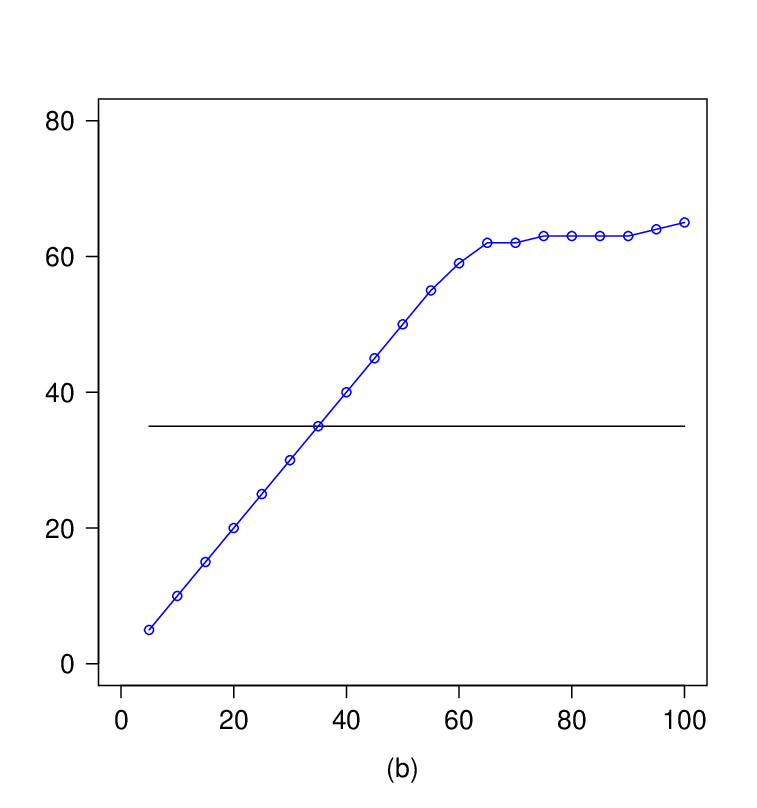
Continuing with this example, we impose additional structure on the terms of $\mathcal{U}$ and choose the last $30$ terms (at random) from the first $70$ terms and give them the exponentially decaying weights in (5.3). Since by the original construction the terms were nearly mutually orthogonal, for double precision accuracy the algorithms should produce $\sim 70$ terms (cf. Figure 5.2), i.e., choose all the linearly independent terms of the tensor.

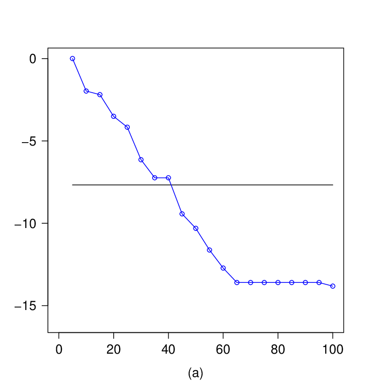
Results for the Gram and randomized tensor ID algorithms are shown in Figure 5.2. The left plot shows the relative $s$ -norm error plotted against the separation rank, $\ell$ , of the tensor IDs computed via the matrices $G$ and $Y$ . The right plot shows the separation rank of the tensor ID approximation as a function of $\ell$ . The underlying separation rank of the CTD is known to be $r\sim 70$ for $\epsilon\sim\epsilon_{machine}$ , and the error for the randomized methods levels off when $k$ approaches this value. The Gram method, however, is only able to identify the first $\sim 35$ terms due to inherent loss of accuracy.

The Frobenius error for the randomized tensor ID approximately matches the $s$ -norm error until the cutoff of $\sqrt{\epsilon_{machine}}$ is attained, at which point it stays constant with respect to $k$ (not shown). Hence, this example also demonstrates the usefulness of the $s$ -norm when high accuracy is sought.

5.2. The tensor ID within convergent, self-correcting Schulz iteration

We present three examples of using the tensor ID within the SGTI approach in order to accelerate reduction of separation rank. These examples were originally presented in [14]. We consider the quadratically convergent, self-correcting Schulz iteration [50], given by

	$\displaystyle\mathbb{X}_{n+1}$	$\displaystyle=$	$\displaystyle 2\mathbb{X}_{n}-\mathbb{X}_{n}\mathbb{B}\mathbb{X}_{n},$
(5.4)		$\displaystyle\mathbb{X}_{0}$	$\displaystyle=$	$\displaystyle\alpha\mathbb{B}^{*},$

where $\alpha$ is chosen so that the initial error $\mathbb{E}_{0}$ satisfies $\left\|\mathbb{E}_{0}\right\|=\left\|\mathbb{I}-\mathbb{X}_{0}\mathbb{B}\right\|<1$ . In these examples, the operator $\mathbb{B}$ is a preconditioned elliptic operator whose inverse corresponds to the Green’s function of a Poisson equation (see more details below). Within each iteration, we first form the quantity $2\mathbb{I}-\mathbb{BX}_{n}$ which we then left-multiply by $\mathbb{X}_{n}$ to obtain $\mathbb{X}_{n+1}$ . Both of these operations significantly increase the separation rank and require a reduction step.

The reduction step, which would typically be performed using ALS, is instead performed with the randomized projection tensor ID Algorithm 3. Only after each complete iteration, when the separation rank has been reduced as much as possible via the tensor ID, is ALS invoked to further refine the approximation. In doing so, we avoid using ALS in the usual manner, i.e., to achieve a certain accuracy of approximation. Instead, its role is limited to reducing the dynamic range of the $s$ -values (i.e., avoiding near cancellation of terms with large $s$ -values) by running the algorithm for only a fixed (small) number of iterations. The reduction errors of the tensor ID and several ALS iterations are then corrected by the next Schulz iteration.

5.2.1. Inverse operator for the Poisson equation

As the first example, we consider the periodic, constant coefficient Poisson equation. In this case we know that the Green’s function has an efficient separated representation, see e.g., [10], and we want to demonstrate that we can approximate the Green’s function starting with the differential operators in

(5.5)		$\displaystyle-\Delta u(\mathbf{x})$	$\displaystyle=$	$\displaystyle f(\mathbf{x}),\,\,\,\,\,\,\,\,\,\,\,\,\mathbf{x}\in(0,1)^{3},$
	$\displaystyle u(0,y,z)$	$\displaystyle=$	$\displaystyle u(0,y,z),$
	$\displaystyle u(x,0,z)$	$\displaystyle=$	$\displaystyle u(x,1,z),$
	$\displaystyle u(x,y,0)$	$\displaystyle=$	$\displaystyle u(x,y,1).$

where

\Delta=\frac{\partial^{2}}{\partial x_{1}^{2}}+\frac{\partial^{2}}{\partial x_{2}^{2}}+\frac{\partial^{2}}{\partial x_{3}^{2}}.

We use eighth-order finite differences to discretize the second derivative in each direction to obtain the $512\times 512$ matrix $A$ , leading to the operator with separation rank $r=3$ ,

\mathbb{A}=A\otimes I\otimes I+I\otimes A\otimes I+I\otimes I\otimes A

where $I$ denotes the identity matrix. We represent the matrix $A$ in a wavelet basis to ensure that both the operator and its inverse are sparse [8, 9, 6, 7]. In a wavelet basis, the second derivative operator has a diagonal preconditioner, $P$ (see e.g., [7]), such that the condition number of $PAP$ is $\mathcal{O}(1)$ . Applying such preconditioner in dimension $d=3$ results in the well-conditioned operator

\mathbb{B}=\left(PAP\right)\otimes I\otimes I+I\otimes\left(PAP\right)\otimes I+I\otimes I\otimes\left(PAP\right).

Since the problem (5.5) is periodic, the operators $\mathbb{A}$ and $\mathbb{B}$ have a one-dimensional null space spanned by a constant. This necessitates the use of the one dimensional projector within the Schulz iteration in order to avoid accumulation of the error in the null space. The results of this computation are shown in Figure 5.3.

5.2.2. Variable coefficient elliptic operator in dimension $d=10$ .

Next we consider the 10-dimensional PDE on the unit cube,

(5.6)

\displaystyle-\nabla\cdot(a(\mathbf{x})\nabla u(\mathbf{x}))

\displaystyle=

\displaystyle f(\mathbf{x}),\,\,\,\,\,\,\,\,\,\,\,\,\mathbf{x}\in(0,1)^{10},

with periodic boundary conditions and where

(5.7)

a(\mathbf{x})=1-0.9\exp\left(-3\times 10^{3}\cdot(\mathbf{x}-0.5)^{2}\right).

In this case we reformulate the problem by using the constant coefficient Green’s function to convert (5.6) into an integral equation, i.e., the constant coefficient Green’s function is used as a preconditioner. By separating the constant from the variable terms in (5.6), the discretized elliptic operator $\mathbb{A}$ can be split into constant and variable parts,

(5.8)

\mathbb{A}=\mathbb{A}_{c}+\mathbb{A}_{v}.

Applying the discretized, constant coefficient Green’s function $\mathbb{G}_{c}$ to $\mathbb{A}$ , we obtain

(5.9)

\mathbb{B}\,=\,\mathbb{G}_{c}\left(\mathbb{A}_{c}+\mathbb{A}_{v}\right)\,\,=\,\,\mathbb{I}+\mathbb{G}_{c}\mathbb{A}_{v}.

The variable coefficient Green’s function $\mathbb{G}$ of equation (5.6) can now be constructed by computing $\mathbb{B}^{-1}$ via Schulz iteration and setting $\mathbb{G}=\mathbb{B}^{-1}\mathbb{G}_{c}$ .

In this example, second order staggered finite differences are used to discretize the derivative operators in each direction at $128$ equispaced points, leading to the elliptical operator $\mathbb{A}$ with separation rank $20$ . Upon applying the constant coefficient Green’s function $\mathbb{G}_{c}$ and truncating terms with small $s$ -values, the preconditioned operator $\mathbb{B}$ has nominal separation rank $271$ . To $6$ digits of relative accuracy, however, the separation rank of $\mathbb{B}$ may be dramatically reduced (via, e.g., ALS iteration), and thus the iteration proceeds on an operator of separation rank only $5$ . As before, we represent all operators in a wavelet basis to ensure the sparsity of both $\mathbb{B}$ and $\mathbb{B}^{-1}$ . Results are shown in Figure 5.4.

5.2.3. Stochastic PDE in dimension $d=8$ .

In our last example, we consider the 8-dimensional stochastic PDE,

-\nabla\cdot(a(\mathbf{x},\omega)\nabla u(\mathbf{x},\omega))=f(\mathbf{x},\omega),\,\,\,\,\,\,\,\,\,\,\mathbf{x}\in(0,1)^{3},

where $\omega\in\Omega$ corresponds to probability space $(\Omega,\mathcal{F},P)$ and the (spatially asymmetric) variable coefficient is given by

a(\mathbf{x},\omega)=1+\sum_{l=1}^{5}2^{-l}a_{l}(\omega)\sin(2l\pi x)\sin(2l\pi y)\sin(2(l+1)\pi z).

In other words, the variable coefficient is understood to have a deterministic spatial part with random coefficients, which we take in this example to be uniformly distributed, $a_{l}\sim U\left(\left[-1,1\right]\right).$ The function $a$ may be thought of as a Karhunen-Loeve (KL) expansion of a random field with some (here, unspecified) covariance function. The resulting operator is thus 8-dimensional, with three spatial and five stochastic dimensions, the latter of which are discretized at Clenshaw-Curtis quadrature nodes,

a_{l}(\omega_{n})=-\cos\left(\frac{\pi m}{M_{stoch}-1}\right),\,\,\,\,\,\,\,l=1,\dots,5,\,\,\,\,\,\,\,m=1,\dots,M_{stoch}-1.

As before, the spatial operator is discretized on a staggered grid at $128$ points using second order finite differences, and we use $M_{stoch}=16$ nodes in the stochastic directions. For the preconditioner, we use the constant coefficient Green’s function in the spatial directions and identity matrices in the stochastic directions, leading to a preconditined operator $\mathbb{B}$ with nominal separation rank of $1188$ . This number is reduced to $24$ by truncating terms with small $s$ -svalues and then applying ALS to the result. Results are shown in Figure 5.5.

5.3. A limitation of tensor ID: orthogonal decompositions

Finally, we illustrate a limitation of using the tensor ID by constructing an example for which it is not expected to work at all. Consider the $d$ -dimensional tensor

(5.10)

\mathcal{U}=\bigotimes_{j=1}^{d}\left(\sum_{l=1}^{L}\sigma_{l}\mathbf{u}_{j}^{(l)}\right)

where $\sigma_{l}=1$ for all $l=1,\dots,L$ , and

(5.11)

\langle\mathbf{u}_{j}^{(l)},\mathbf{u}_{j}^{(m)}\rangle=\delta_{lm}

for $j=1,\dots,d$ and $l,m=1,\dots L$ . Objects such as (5.10) appear quite frequently in various fields. For example, if we take the vectors $\mathbf{u}_{j}^{(l)}$ to correspond to orthogonal polynomials with respect to a specified probability measure, discretized at properly chosen quadrature nodes, $\mathcal{U}$ may be interpreted as a tensor order polynomial chaos expansion (PCE) [54].

Expanding the tensor product (5.10), the result is seen to have nominal separation rank $L^{d}$ . By (5.11), all of the terms are mutually orthogonal and, thus, the columns of corresponding matrix $U$ in (1.11) are orthonormal. Consequently, the tensor ID cannot provide a reduction of the separation rank. However, if the $s$ -values decay rapidly, we can truncate with controlled error by using Parseval’s identity (cf., Example 5.1). In fact, truncation may in this case be viewed as a special instance of the tensor ID, with skeleton indices corresponding to the $k$ terms with $s$ -values above the accuracy threshold.

Acknowledgements

We would like to thank Martin Mohlenkamp (Ohio University) and Terry Haut (LANL) for making many useful suggestions to improve the manuscript.

References

[1] E. Acar and B. Yener. Unsupervised multiway data analysis: A literature survey. Knowledge and Data Engineering, IEEE Transactions on, 21(1):6–20, 2009.
[2] D. Achlioptas. Database-friendly random projections: Johnson-Lindenstrauss with binary coins. J. Comput. Syst. Sci., 66(4):671–687, June 2003.
[3] D. Achlioptas and F. Mcsherry. Fast computation of low-rank matrix approximations. Journal of the ACM (JACM), 54(2):9, 2007.
[4] N. Ailon and B. Chazelle. Approximate nearest neighbors and the fast Johnson-Lindenstrauss transform. In Proceedings of the thirty-eighth annual ACM symposium on Theory of computing, pages 557–563. ACM, 2006.
[5] B. W. Bader and T. G. Kolda. Matlab Tensor Toolbox Version 2.5. Available online, January 2012.
[6] G. Beylkin. On the representation of operators in bases of compactly supported wavelets. SIAM J. Numer. Anal., 29(6):1716–1740, 1992.
[7] G. Beylkin. On wavelet-based algorithms for solving differential equations. In J. J. Benedetto and M. W. Frazier, editors, Wavelets: mathematics and applications, Stud. Adv. Math., pages 449–466. CRC, Boca Raton, FL, 1994.
[8] G. Beylkin, R. Coifman, and V. Rokhlin. Fast wavelet transforms and numerical algorithms, I. Comm. Pure Appl. Math., 44(2):141–183, 1991. Yale Univ. Technical Report YALEU/DCS/RR-696, August 1989.
[9] G. Beylkin, R. Coifman, and V. Rokhlin. Wavelets in numerical analysis. In Wavelets and their applications, pages 181–210. Jones and Bartlett, Boston, MA, 1992.
[10] G. Beylkin, G. Fann, R. J. Harrison, C. Kurcz, and L. Monzón. Multiresolution representation of operators with boundary conditions on simple domains. Appl. Comput. Harmon. Anal., 33:109–139, 2012. http://dx.doi.org/10.1016/j.acha.2011.10.001.
[11] G. Beylkin, J. Garcke, and M. J. Mohlenkamp. Multivariate regression and machine learning with sums of separable functions. SIAM Journal on Scientific Computing, 31(3):1840–1857, 2009.
[12] G. Beylkin and M. J. Mohlenkamp. Numerical operator calculus in higher dimensions. Proc. Natl. Acad. Sci. USA, 99(16):10246–10251, August 2002.
[13] G. Beylkin and M. J. Mohlenkamp. Algorithms for numerical analysis in high dimensions. SIAM J. Sci. Comput., 26(6):2133–2159, July 2005.
[14] D. Biagioni. Numerical Construction of Green’s Functions in High-dimensional Elliptic Problems with Variable Coefficients and Analysis of Renewable Energy Data via Sparse and Separable Approximations. PhD thesis, University of Colorado, 2012.
[15] R. Bro. Parafac. Tutorial & Applications. In Chemom. Intell. Lab. Syst., Special Issue 2nd Internet Conf. in Chemometrics (incinc’96), volume 38, pages 149–171, 1997. http://www.models.kvl.dk/users/rasmus/presentations/parafac_tutorial/paraf.htm.
[16] E. J. Candès and T. Tao. Near-optimal signal recovery from random projections: universal encoding strategies? IEEE Trans. Inform. Theory, 52(12):5406–5425, 2006.
[17] E.J. Candès, J. Romberg, and T. Tao. Robust uncertainty principles: exact signal reconstruction from highly incomplete frequency information. Information Theory, IEEE Transactions on, 52(2):489 – 509, feb. 2006.
[18] J. D. Carroll and J. J. Chang. Analysis of individual differences in multidimensional scaling via an N-way generalization of Eckart-Young decomposition. Psychometrika, 35:283–320, 1970.
[19] H. Cheng, Z. Gimbutas, P.-G. Martinsson, and V. Rokhlin. On the compression of low-rank matrices. SIAM Journal of Scientific Computing, 205(1):1389–1404, 2005.
[20] W. F. de la Vega, M. Karpinski, R. Kannan, and S. Vempala. Tensor decomposition and approximation schemes for constraint satisfaction problems. In Proceedings of the thirty-seventh annual ACM symposium on Theory of computing, STOC ’05, pages 747–754, New York, NY, USA, 2005. ACM.
[21] L. De Lathauwer, B. De Moor, and J. Vandewalle. On the best rank-1 and rank-(r1,r2,. . .,rn) approximation of higher-order tensors. SIAM J. Matrix Anal. Appl., 21(4):1324–1342, 2000.
[22] V. de Silva and L.-H. Lim. Tensor rank and the ill-posedness of the best low-rank approximation problem. SIAM J. Matrix Anal. Appl., 30(3):1084–1127, 2008.
[23] J. Demmel. Accurate singular value decompositions of structured matrices. SIAM J. Matrix Anal. Appl., 21(2):562–580, 1999.
[24] P. Drineas and R. Kannan. Pass efficient algorithms for approximating large matrices. In Proceedings of the fourteenth annual ACM-SIAM symposium on Discrete algorithms, SODA ’03, pages 223–232, Philadelphia, PA, USA, 2003. Society for Industrial and Applied Mathematics.
[25] P. Drineas and M. W. Mahoney. A randomized algorithm for a tensor-based generalization of the Singular Value Decomposition. Linear Algebra Appl., 420(2-3):553–571, 2007.
[26] A. Frieze, R. Kannan, and S. Vempala. Fast Monte-Carlo algorithms for finding low-rank approximations. J. ACM, 51(6):1025–1041, November 2004.
[27] Sergei A Goreinov, Eugene E Tyrtyshnikov, and Nickolai L Zamarashkin. A theory of pseudoskeleton approximations. Linear Algebra and its Applications, 261(1):1–21, 1997.
[28] Sergei A Goreinov, Nikolai Leonidovich Zamarashkin, and Evgenii Evgen’evich Tyrtyshnikov. Pseudo-skeleton approximations by matrices of maximal volume. Mathematical Notes, 62(4):515–519, 1997.
[29] L. Grasedyck, D. Kressner, and C. Tobler. A literature survey of low-rank tensor approximation techniques. CoRR, abs/1302.7121, 2013.
[30] Ming Gu and Stanley C Eisenstat. Efficient algorithms for computing a strong rank-revealing qr factorization. SIAM Journal on Scientific Computing, 17(4):848–869, 1996.
[31] N. Halko, P.-G. Martinsson, and J. A. Tropp. Finding structure with randomness: probabilistic algorithms for constructing approximate matrix decompositions. SIAM Review, 53(2):217–288, 2011.
[32] R. A. Harshman. Foundations of the Parafac procedure: model and conditions for an “explanatory” multi-mode factor analysis. Working Papers in Phonetics 16, UCLA, 1970. http://publish.uwo.ca/ $\sim$ harshman/wpppfac0.pdf.
[33] C. Hillar and L.-H. Lim. Most tensor problems are NP hard. Technical Report arXiv:0911.1393, Nov 2009.
[34] W. B. Johnson and J. Lindenstrauss. Extensions of Lipschitz mappings into a Hilbert space. In Conference in modern analysis and probability (New Haven, Conn., 1982), volume 26 of Contemp. Math., pages 189–206. Amer. Math. Soc., Providence, RI, 1984.
[35] E. Kofidis and P. A. Regalia. On the best rank-1 approximation of higher-order supersymmetric tensors. SIAM J. Matrix Anal. Appl., 23(3):863–884, 2001.
[36] T. G. Kolda and B. W. Bader. Tensor decompositions and applications. SIAM Review, 51(3):455–500, 2009.
[37] T. G. Kolda and J. R. Mayo. Shifted power method for computing tensor eigenpairs. SIAM Journal on Matrix Analysis and Applications, 32(4):1095–1124, October 2011.
[38] E. Liberty, F. Woolfe, P-G. Martinsson, V. Rokhlin, and M. Tygert. Randomized algorithms for the low-rank approximation of matrices. Proc. Natl. Acad. Sci. USA, 104(51):20167–20172, 2007.
[39] L.-H. Lim. Singular values and eigenvalues of tensors: a variational approach. In Computational Advances in Multi-Sensor Adaptive Processing, 2005 1st IEEE International Workshop on, pages 129–132, 2005.
[40] M. W. Mahoney. Tensor-cur decompositions for tensor-based data. In In Proceedings of the 12th Annual ACM SIGKDD Conference, pages 327–336, 2006.
[41] P-G. Martinsson, V. Rokhlin, and M. Tygert. A randomized algorithm for the approximation of matrices. Technical report, Yale CS research report YALEU/DCS/RR-1361, 2006.
[42] P.-G. Martinsson, V. Rokhlin, and M. Tygert. A randomized algorithm for the approximation of matrices. Applied and Computational Harmonic Analysis, 30(1):47–68, 2011.
[43] MATLAB. Version 8.0.0 (R2012b). The MathWorks Inc., Natick, Massachusetts, 2012.
[44] Martin J Mohlenkamp. Musings on multilinear fitting. Linear Algebra and its Applications, 438:834–852, 2011.
[45] N. H Nguyen, P. Drineas, and T. D Tran. Tensor sparsification via a bound on the spectral norm of random tensors. arXiv preprint arXiv:1005.4732, 2010.
[46] C. H. Papadimitriou, H. Tamaki, P. Raghavan, and S. Vempala. Latent semantic indexing: a probabilistic analysis. In Proceedings of the seventeenth ACM SIGACT-SIGMOD-SIGART symposium on Principles of database systems, PODS ’98, pages 159–168, New York, NY, USA, 1998. ACM.
[47] H. Rauhut, R. Schneider, and Z. Stojanac. Low-rank tensor recovery via iterative hard thresholding. In Proceedings of the International Conference on Sampling Theory and Applications (preprint), 2013.
[48] M. Rudelson and R. Vershynin. Sampling from large matrices: An approach through geometric functional analysis. J. ACM, 54(4), July 2007.
[49] T. Sarlos. Improved approximation algorithms for large matrices via random projections. In Foundations of Computer Science, 2006. FOCS ’06. 47th Annual IEEE Symposium on, pages 143–152, 2006.
[50] G. Schulz. Iterative Berechnung der reziproken Matrix. Z. Angew. Math. Mech., 13:57–59, 1933.
[51] G. Tomasi and R. Bro. A comparison of algorithms for fitting the PARAFAC model. Comput. Statist. Data Anal., 50(7):1700–1734, 2006.
[52] C. E. Tsourakakis. Mach: Fast randomized tensor decompositions. CoRR, abs/0909.4969, 2009.
[53] Eugene Tyrtyshnikov. Mosaic-skeleton approximations. Calcolo, 33(1-2):47–57, 1996.
[54] N. Wiener. The Homogeneous Chaos. American Journal of Mathematics, 60(4):897–936, 1938.
[55] F. Woolfe, E. Liberty, V. Rokhlin, and M. Tygert. A fast randomized algorithm for the approximation of matrices. Appl. Comput. Harmon. Anal., 25(3):335–366, 2008.
[56] T. Zhang and G. H. Golub. Rank-one approximation to high order tensors. SIAM J. Matrix Anal. Appl., 23(2):534–550, 2001.

6. Online supplement

6.1. Proof of Theorem 3.1

Lemma 6.1.

Suppose that $B_{k}=B_{c}P$ is a rank- $k$ interpolative decomposition of $B$ . Then

(6.1)

B_{k}=A^{*}A_{c}P.

Proof.

By definition, we have that

(6.2)

[B]_{ll^{\prime}}=[A^{*}A]_{ll^{\prime}}=\langle\mathbf{a}^{(l)},\mathbf{a}^{(l^{\prime})}\rangle,\,\,\,l,l^{\prime}=1,\dots,n,

where $\mathbf{a}^{(l)}$ denotes the column $l$ of $A$ . Thus, the column skeleton of $B$ is of the form

(6.3)

[B_{c}]_{lj}=\langle\mathbf{a}^{(l)},\mathbf{a}^{(l_{j}^{\prime})}\rangle,\,\,\,\,j=1,\dots,k,

where indices $l_{j}^{\prime}$ are those of the skeleton columns of $B$ ; we denote this subset as $\mathcal{L}_{k}$ . We have

[B_{k}]_{ll^{\prime}}=\sum_{j=1}^{k}[B_{c}]_{lj}[P]_{jl^{\prime}}=\sum_{j=1}^{k}\langle\mathbf{a}^{(l)},\mathbf{a}^{(l^{\prime}_{j})}\rangle[P]_{jl^{\prime}}=\langle\mathbf{a}^{(l)},\sum_{j=1}^{k}\mathbf{a}^{(l^{\prime}_{j})}[P]_{jl^{\prime}}\rangle=[A^{*}A_{c}P]_{ll^{\prime}}

∎

Lemma 6.2.

Suppose $B$ is a symmetric matrix that admits a rank- $k$ interpolative decomposition $\hat{B}_{k}=B_{c}\hat{P}$ such that

(6.4)

\left\|B-\hat{B}_{k}\right\|_{2}\leq\epsilon_{k}.

Then it also admits a decomposition of the form

(6.5)

\hat{B}_{k}=P^{*}B_{s}\hat{P},

with identical error. Symmetrizing with respect to $P=\left[\begin{array}[]{c|c}I&S\end{array}\right]$ , i.e., setting

(6.6)

B_{k}=P^{*}B_{s}P,

this approximation satisfies

(6.7)

\left\|B-B_{k}\right\|_{2}\leq(1+\sqrt{nk(n-k)})\epsilon_{k}.

Proof.

Define the $n\times n$ matrix $Y=B-B_{k}.$ Following the proof of Theorem 3 in [19], we first compute a pivoted QR factorization of $B$ such that

(6.8)

BP_{c}=QR,

where the $n\times k$ matrix $Q$ has orthonormal columns, $R$ is a $k\times n$ upper triangular matrix, and $P_{c}$ is an $n\times n$ permutation matrix. We label blocks of the matrices $Q$ and $R$ as

(6.9)

Q=\left[\begin{array}[]{c|c}Q_{11}&Q_{12}\\ \hline\cr Q_{21}&Q_{22}\end{array}\right],\,\,\,\,\,\,\,\,\,R=\left[\begin{array}[]{c|c}R_{11}&R_{12}\\ \hline\cr 0&R_{22}\end{array}\right].

Here the blocks of $Q$ have the following dimensions dimensions: $Q_{11}$ is $k\times k$ , $Q_{12}$ is $k\times(n-k)$ , $Q_{21}$ is $(n-k)\times k$ and $Q_{22}$ is $(n-k)\times(n-k)$ . The blocks of $R$ have the corresponding dimensions so that the product $QR$ may be expressed in terms of the products of blocks. We set (as in [19])

(6.10)

B_{c}=\left[\begin{array}[]{c}Q_{11}R_{11}\\ \hline\cr Q_{21}R_{11}\end{array}\right],

so that $B=B_{c}\hat{P}+Y,$ where

(6.11)

Y=\left[\begin{array}[]{c|c}0&Q_{12}\\ \hline\cr 0&Q_{22}\end{array}\right]R_{22}P_{c}^{*},

and

(6.12)

\hat{P}=\left[\begin{array}[]{c|c}I&T\end{array}\right]P_{c}^{*}

and $T$ the least squares solution of $R_{11}T=R_{12}$ ( $T$ may not be unique if $R_{11}$ is ill-conditioned).

Since $B$ is symmetric, a suitable basis for the column space of $B$ is also a suitable basis for the row space. We compute the QR decomposition of $B_{c}^{*}P_{c}^{*}$ (without pivoting),

(6.13)

B_{c}^{*}P_{c}^{*}=\tilde{Q}\left[\begin{array}[]{c|c}\tilde{R}_{11}&\tilde{R}_{12}\end{array}\right]

and notice that the blocks $\tilde{R}_{21}$ and $\tilde{R}_{22}$ are zero since $B_{c}$ has exactly rank $k$ . Since $B_{CS}=A^{*}A_{c}$ , using Lemma 6.1 we have

(6.14)

B_{c}^{*}P_{c}^{*}=A_{c}^{*}\left[\begin{array}[]{c|c}A_{c}&\hat{A}\end{array}\right],

where the $n\times(n-k)$ block $\hat{A}$ consist of the non-skeleton columns of $A$ . Because the columns have been already pivoted, it follows that

	$\displaystyle\tilde{Q}\tilde{R}_{11}$	$\displaystyle=$	$\displaystyle A_{c}^{*}A_{c}$
(6.15)		$\displaystyle\tilde{Q}\tilde{R}_{12}$	$\displaystyle=$	$\displaystyle A_{c}^{*}\hat{A}.$

Finally, again following [19], we have

(6.19)		$\displaystyle B$	$\displaystyle=$	$\displaystyle P_{c}\left[\begin{array}[]{c}I\\ \hline\cr\tilde{R}_{12}^{}(\tilde{R}_{11}^{})^{-1}\end{array}\right]\tilde{R}_{11}^{}\tilde{Q}^{}P+Y$
(6.19)			$\displaystyle=$	$\displaystyle P^{*}B_{s}\hat{P}+Y$

where $B_{s}=A_{c}^{*}A_{c}$ is the skeleton of $B$ ,

(6.20)

P=\left[\begin{array}[]{c|c}I&S\end{array}\right]P_{c}^{*}.

and $S$ is a least squares solution of

(6.21)

\displaystyle S\tilde{R}_{11}^{*}

\displaystyle=

\displaystyle\tilde{R}_{12}^{*}.

satisfying

(6.22)

\left\|S\right\|_{2}\leq\sqrt{nk(n-k)}.

Notice that the error is unchanged upon factorization of the row space. This proves the first claim.

To prove the second claim, notice first that the left (row) coefficient matrix $S$ solves

(6.23)

A_{c}^{*}A_{c}S-A_{c}^{*}\hat{A}=0,

while the right (column) coefficient matrix $T$ solves

(6.24)

\left[\begin{array}[]{c}A_{c}^{*}A_{c}\\ \hline\cr\hat{A}^{*}A_{c}\end{array}\right]T=\left[\begin{array}[]{c}A_{c}^{*}\hat{A}\\ \hline\cr\hat{A}^{*}\hat{A}\end{array}\right]

approximately, such that

	$\displaystyle\left\\|A_{c}^{}A_{c}T-A_{c}^{}\hat{A}\right\\|_{2}$	$\displaystyle\leq$	$\displaystyle\epsilon_{k},$
(6.25)		$\displaystyle\bigl\\|\hat{A}^{}A_{c}T-\hat{A}^{}\hat{A}\bigr\\|_{2}$	$\displaystyle\leq$	$\displaystyle\epsilon_{k}.$

The quantity of interest is $B-\tilde{B}_{k}$ , which we permute so that the skeleton columns are in the first $k$ positions, giving

	$\displaystyle P_{c}^{}\left(B-P^{}B_{s}P\right)P_{c}$	$\displaystyle=$	$\displaystyle\left[\begin{array}[]{c}A_{c}^{}\\ \hline\cr\hat{A}^{}\end{array}\right]\left[\begin{array}[]{c\|c}A_{c}&\hat{A}\end{array}\right]-\left[\begin{array}[]{c}I\\ \hline\cr S^{}\end{array}\right]A_{c}^{}A_{c}\left[\begin{array}[]{c\|c}I&S\end{array}\right]$
		$\displaystyle=$	$\displaystyle\left[\begin{array}[]{c\|c}0&0\\ \hline\cr 0&\hat{A}^{}\hat{A}-S^{}A_{c}^{*}A_{c}S\end{array}\right]$

where the off-diagonal blocks are set to zero by virtue of the fact that $S$ solves the normal equations exactly. Adding and subtracting $S^{*}A_{c}^{*}A_{c}T$ to the non-zero block, we have

(6.36)	$\displaystyle\bigl\\|\hat{A}^{}\hat{A}-S^{}A_{c}^{*}A_{c}S\bigr\\|_{2}$	$\displaystyle=$	$\displaystyle\bigl\\|\hat{A}^{}\hat{A}-S^{}B_{s}S+S^{}B_{s}T-S^{}B_{s}T\bigr\\|_{2}$
		$\displaystyle\leq$	$\displaystyle\bigl\\|\hat{A}^{}\hat{A}-S^{}B_{s}T\bigr\\|_{2}+\bigl\\|S^{}B_{s}S-S^{}B_{s}T\bigr\\|_{2}$
		$\displaystyle\leq$	$\displaystyle\epsilon_{k}+\bigl\\|S^{}B_{s}S-S^{}B_{s}T\bigr\\|_{2}$

where the second line follows from the triangle inequality and the third from (6.25). Adding and subtracting $S^{*}A_{c}^{*}\hat{A}$ , we have

(6.37)	$\displaystyle\bigl\\|S^{}B_{s}S-S^{}B_{s}T\bigr\\|_{2}$	$\displaystyle=$	$\displaystyle\bigl\\|(S^{}B_{s}S-S^{}A_{c}^{}\hat{A})-(S^{}B_{s}T-S^{}A_{c}^{}\hat{A})\bigr\\|_{2}$
		$\displaystyle\leq$	$\displaystyle\bigl\\|S\bigr\\|_{2}\left(\bigl\\|B_{s}S-A_{c}\hat{A}\bigr\\|_{2}+\bigl\\|B_{s}T-A_{c}^{*}\hat{A}\bigr\\|_{2}\right)$
		$\displaystyle\leq$	$\displaystyle\bigl\\|S\bigr\\|_{2}\epsilon_{k}$

by the triangle inequality, (6.23) and (6.25). Hence, applying (6.22), we conclude

(6.38)

\bigl\|B-B_{k}\bigr\|_{2}\leq(1+\bigl\|S\bigr\|_{2})\epsilon_{k}\leq(1+\sqrt{nk(n-k)})\epsilon_{k}.

∎

Corollary 6.3.

The coefficient matrix $P$ in (6.20) solves the normal equations

(6.39)

\displaystyle A_{c}^{*}A_{c}P

\displaystyle=

\displaystyle A_{c}^{*}A.

and, thus, minimizes the residual error

(6.40)

\left\|A_{c}P-A\right\|_{2}.

Setting $A_{k}=A_{c}P$ , it follows that the residual $X=A-A_{k}$ is in the null space of $A_{k}^{*}$ .

Proof.

We first note that, in order for a matrix $\tilde{S}$ to minimize

(6.41)

\left\|A_{c}\tilde{S}-\hat{A}\right\|_{2},

it must solve the normal equations (6.39). From (6.15), applying the (pivot-free) QR algorithm to this system yields $A_{c}^{*}A_{c}=\tilde{Q}\tilde{R}_{11}$ and $A_{c}^{*}\hat{A}=\tilde{Q}\tilde{R}_{12}$ , and so

(6.42)

\displaystyle\tilde{Q}\tilde{R}_{11}\tilde{S}

\displaystyle=

\displaystyle\tilde{S}\tilde{Q}\tilde{R}_{12}\,\,\,\,\,\,\,\,\,\Rightarrow\,\,\,\,\,\,\,\,\,\,\tilde{S}\,=\,\tilde{R}_{11}^{-1}\tilde{R}_{12}.

Thus $\tilde{S}=S$ in Lemma 6.2. Since $P=\left[\begin{array}[]{c|c}I&S\end{array}\right]P_{c}^{*}$ , the normal equations (6.39) may be augmented to include the skeleton columns without increasing the error (the projection is exact for these columns).

The second claim follows from the fact that $P$ minimizes (6.40).∎

Remark 6.4.

It is emphatically not the case that replacing $P$ with the the column-oriented matrix $\hat{P}$ in Corollary 6.3 leads to the same result. In fact, in light of (6.24) and (6.25), it will generally not be true that $\hat{P}$ solves the normal equations (6.39).

To complete the proof of the theorem,

Lemma 6.5.

Suppose that the column-oriented interpolative decomposition $\hat{B}_{k}=B_{c}\hat{P}$ satisfies $\bigl\|B-\hat{B}_{k}\bigr\|_{2}\leq\epsilon_{k},$ with $\hat{P}$ defined in (6.12), and $B_{k}=P^{*}B_{s}P$ is its symmetrized version with $P$ defined in (6.20). Setting $A_{k}=A_{c}P$ , we have

(6.43)

\left\|A-A_{k}\right\|_{2}=\left\|B-B_{k}\right\|_{2}^{1/2}\leq\left((1+\sqrt{nk(n-k)})\epsilon_{k}\right)^{1/2}.

Proof.

That a symmetric decomposition exists follow from Lemma 6.2. Formally, let the QR factorization of $A_{k}$ be given by

(6.44)

A_{k}=Q_{k}R_{k}

where $Q_{k}$ is a $m\times k$ matrix with orthogonal columns and $R_{k}$ is a $k\times n$ upper rectangular matrix. By Corollary 6.3, the orthogonal projector defined by $Q_{k}Q_{k}^{*}$ coincides with the matrix $P$ in the sense that

(6.45)

\displaystyle A_{k}\,\,=\,\,A_{c}P

\displaystyle=

\displaystyle Q_{k}Q_{k}^{*}A.

Next, define the residual

(6.46)

X=A-A_{k}

and decompose it via $X=X_{1}+X_{2}$ , where

(6.47)

\begin{array}[]{ccc}X_{1}=Q_{k}Q_{k}^{*}X,&&X_{2}=(I-Q_{k}Q_{k}^{*})X.\end{array}

By Corollary 6.3, we have that $X_{1}=0$ , and so $A=A_{k}+X_{2}$ with $X_{2}$ in the null space of $A_{k}^{*}$ . In addition,

(6.48)

\displaystyle B_{k}

\displaystyle=

\displaystyle A_{k}^{*}A_{k}\,\,=\,\,(Q_{k}Q_{k}^{*}A)^{*}(Q_{k}Q_{k}^{*}A)\,\,=\,\,A^{*}Q_{k}Q_{k}^{*}A.

Thus

(6.49)		$\displaystyle B-B_{k}$	$\displaystyle=$	$\displaystyle A^{}A-A^{}Q_{k}Q_{k}^{}A\,\,=\,\,(A-Q_{k}Q_{k}^{}A)^{}(A-Q_{k}Q_{k}^{}A)$
(6.49)			$\displaystyle=$	$\displaystyle(A-A_{k})^{*}(A-A_{k}).$

Hence, $\left\|A-A_{k}\right\|_{2}=\left\|B-B_{k}\right\|_{2}^{1/2}$ , with the upper bound $\left((1+\sqrt{nk(n-k)})\epsilon_{k}\right)^{1/2}$ following directly from Lemma 6.2.∎

	$\displaystyle P_{c}^{}\left(B-P^{}B_{s}P\right)P_{c}$	$\displaystyle=$	$\displaystyle\left[\begin{array}[]{c}A_{c}^{}\\ \hline\cr\hat{A}^{}\end{array}\right]\left[\begin{array}[]{c\|c}A_{c}&\hat{A}\end{array}\right]-\left[\begin{array}[]{c}I\\ \hline\cr S^{}\end{array}\right]A_{c}^{}A_{c}\left[\begin{array}[]{c\|c}I&S\end{array}\right]$
		$\displaystyle=$	$\displaystyle\left[\begin{array}[]{c\|c}0&0\\ \hline\cr 0&\hat{A}^{}\hat{A}-S^{}A_{c}^{*}A_{c}S\end{array}\right]$

Abstract.

Key words and phrases:

1. Introduction

1.1. Definitions and notation.

Remark 1.1.

1.2. Tensor interpolative decomposition

1.3. Contributions and relationship to prior work

2. Preliminaries

2.1. Randomized algorithm for approximating the range of a matrix

Theorem 2.1.

2.2. Interpolative matrix decomposition

Lemma 2.2.

Remark 2.3.

2.3. A randomized algorithm for interpolative matrix decomposition

Lemma 2.4.

Remark 2.5.

2.4. Q-factorization for tensors

Lemma 2.6.

3. Randomized Tensor Interpolative Decomposition

3.1. On the interpolative decomposition of symmetric matrices

Theorem 3.1.

Remark 3.2.

3.2. Tensor ID problem

Theorem 3.3.

Lemma 3.4.

Proof.

Theorem 3.5.

Proof.

Remark 3.6.

3.3. Projection algorithm with random tensors in canonical form

3.3.1. Random tensors in canonical form

3.3.2. Cost estimate

3.3.3. Comparison of computational costs

4. Frobenius norm and ss-norm of a tensor

Lemma 4.1.

Proof.

Remark 4.2.

Lemma 4.3.

Proof.

4.1. Approximating the ss-norm

5. Examples

5.1. Comparison of matrices associated with tensor ID algorithms

5.2. The tensor ID within convergent, self-correcting Schulz iteration

5.2.1. Inverse operator for the Poisson equation

5.2.2. Variable coefficient elliptic operator in dimension d=10d=10.

5.2.3. Stochastic PDE in dimension d=8d=8.

5.3. A limitation of tensor ID: orthogonal decompositions

Acknowledgements

References

6. Online supplement

6.1. Proof of Theorem 3.1

Lemma 6.1.

Proof.

Lemma 6.2.

Proof.

Corollary 6.3.

Proof.

Remark 6.4.

Lemma 6.5.

Proof.

4. Frobenius norm and $s$ -norm of a tensor

4.1. Approximating the $s$ -norm

5.2.2. Variable coefficient elliptic operator in dimension $d=10$ .

5.2.3. Stochastic PDE in dimension $d=8$ .