Parametrizing the exoplanet eccentricity distribution with the Beta distribution
Abstract
It is suggested that the distribution of orbital eccentricities for extrasolar planets is well-described by the Beta distribution. Several properties of the Beta distribution make it a powerful tool for this purpose. For example, the Beta distribution can reproduce a diverse range of probability density functions (PDFs) using just two shape parameters ( and ). We argue that this makes it ideal for serving as a parametric model in Bayesian comparative population analysis. The Beta distribution is also uniquely defined over the interval zero to unity, meaning that it can serve as a proper prior for eccentricity when analysing the observations of bound extrasolar planets. Using nested sampling, we find that the distribution of eccentricities for 396 exoplanets detected through radial velocity with high signal-to-noise is well-described by a Beta distribution with parameters and . The Beta distribution is shown to be 3.7 times more likely to represent the underlying distribution of exoplanet eccentricities than the next best model: a Rayleigh + exponential distribution. The same data are also used in an example population comparison utilizing the Beta distribution, where we find that the short- and long-period planets are described by distinct Beta distributions at a confidence of 11.6 and display a signature consistent with the effects of tidal circularization.
Keywords:
methods: statistical — planets and satellites: general1 Introduction
Thanks to the tireless efforts of observers in recent years, there now exists a sizeable library of orbital eccentricities () for extrasolar planets. Although photometric techniques are starting to emerge for measuring , such as Multibody Asterodensity Profiling (MAP) (Kipping et al., 2012), the precise determination of this quantity has been historically determined by the radial velocity variations (RV) of the host stars.
This library of values has several uses and we focus on two particularly useful applications here. The first is that the distribution can be exploited to test and refine theories of planet formation and evolution and offers a window into the possible scattering history of planetary systems (Rasio & Ford, 1996; Jurić & Tremaine, 2008; Chatterjee et al., 2008). Such tests typically operate by taking a theoretical prediction for the distribution of various exoplanet parameters, in particular , and comparing to the measured distribution from, say, RV surveys. This comparison of distributions can also be extended to subpopulations of exoplanets, such as seeking evidence of tidal circularization by comparing the distribution of between short- and long-period planets. To make a quantitative comparison, one may use the popular non-parametric and frequentist Kolmogorov-Smirnov (KS) test between the two populations. Alternatively, a parametric approach (useful for Bayesian analyses) would be to regress one or more analytic distributions to the observed one. The parameters describing the analytic distribution may then be compared to test for statistically significant differences, or lack thereof.
A second useful application of an observed eccentricity distribution is that it can be used to derive an informative prior on eccentricities in general. Before the availability of this information, observers have been forced to adopt uninformative priors, typically being a uniform prior over , but an informative prior can be preferable in many situations. Some examples we consider are fitting RV data with phase gaps (which can lead to spurious eccentricities), non-detection radial velocities used to place upper limits on (e.g. Kepler-22b; Borucki et al. 2012), blend analyses of transits requiring some eccentricity prior (Fressin et al., 2011) and fitting transit light curves with an absence of any empirical eccentricity constraints. Using an informative prior naturally includes an observer’s experience of the known distribution, taking into account whether a particular solution is a surprisingly rare answer or a very typical one. Any prior of course requires a parametrization of the observed eccentricity distribution. Furthermore, for use as a prior, the distribution should not reproduce negative eccentricities or hyperbolic orbits (since any periodic transit, RV, asterometric, etc. signal cannot result from such an orbit) and should integrate to unity over the range to be defined as a proper prior.
From the aforementioned two major applications of the eccentricity distribution, we identify the following key requirements for any such parametrized probability density function (PDF), :
-
should be defined over the range only i.e. no hyperbolic orbits or negative eccentricities
-
For a proper prior we require i.e. the distribution is normalized over the defined range
-
We require to be able to reproduce a wide range of plausible distributions and be as efficient as possible i.e. use few parameters
-
The inverse of the cumulative density function (CDF) may be easily computed to serve as a practical (i.e. computationally efficient) prior for direct sampling
2 The Beta Distribution
2.1 Properties
The Beta distribution, , is a member of the exponential family defined over the range and satisfies all of the desired criteria described in the previous section. The functional form is expressed in terms of either Gamma functions, or equivalently the Beta function, as
| (1) |
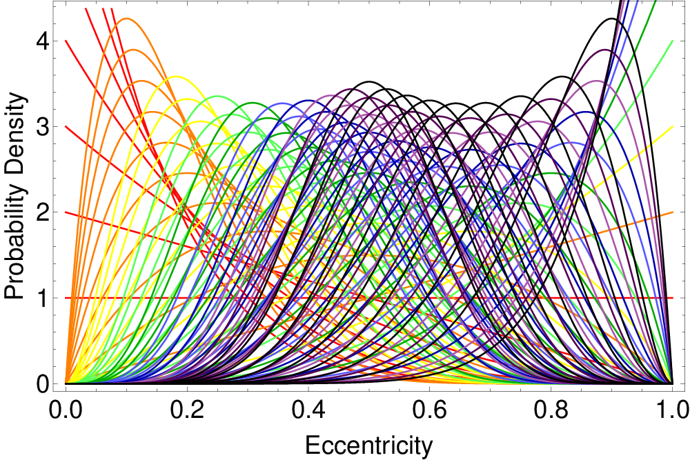
The first advantage of this form is that despite being described by just two parameters, is able to produce a wide and diverse range of probability distributions, as illustrated in Fig. 1. Secondly, the fact that the distribution is defined over the range zero to unity means it is suitable as a proper prior and it is trivial to show that
| (2) |
Thirdly, is clearly efficient given that only two parameters ( and ) reproduce the wide range of distributions illustrated in Fig. 1. Finally, it may be shown that the CDF may be inverted as a stable function, which is a requirement for using the Beta distribution as a prior via direct sampling. The CDF is given by
| (3) |
The inverse function is simply expressed . A Beta distribution prior can therefore be invoked by generating as a random uniform number between zero and unity and computing , thus directly sampling from the prior distribution. This inverse function is widely available in standard programming libraries. We note that Hogg et al. (2010) used a Beta distribution to model the eccentricity distribution of a synthetic population but did not discuss how well the distribution matches the observed distribution nor its potential as a prior.
2.2 Comparison to other commonly used distributions
One of the most commonly used PDFs for modelling the distribution of exoplanet eccentricities is a mixture between a Rayleigh distribution and an exponential distribution (e.g. Steffen et al. 2010; Wang & Ford 2011; Kipping et al. 2012). The appeal of this mixture is that Rayleigh scattering reflects the effects of planet-planet scattering and the exponential component reflects the effects of tidal dissipation (Rasio & Ford, 1996). The associated PDF is
| (4) |
where gives the relative contributions of the two PDFs, is the width parameter of the exponential distribution and is the scale parameter of the Rayleigh distribution.
A major problem with the distribution of equation 4 is that hyperbolic orbits () have a non-zero probability. This is true for both the Rayleigh and exponential components taken individually too. Hyperbolic orbits (i.e. ejected planets) surely do naturally result from planet-planet scattering and planet-synthesis simulations may benefit from using this distribution (Rasio & Ford, 1996). However, it is not appropriate to use such a distribution as a prior for fitting, say, the RV time series of an exoplanet. This is because the very fact that a periodic planet signal has been observed precludes .
Wang & Ford (2011) also used a uniform + exponential distribution to serve as a null-hypothesis against the presence of a Rayleigh + exponential distribution. As before, for the purpose of serving as a prior in fitting, the exponential component will reproduce unobservable scenarios.
Another example of a model used recently for exoplanet eccentricities comes from Shen & Turner (2008) (hereafter ST08), who used a PDF requiring two shape parameters, and .
| (5) |
It is easily shown that this distribution is not uniquely defined over the interval .
3 Example Regressions
3.1 Regressing all planets
Regressing a PDF to a histogram of eccentricities is precarious in that the results are sensitive to the chosen bin sizes. A more robust approach is to regress to the CDF which can be calculated at the smallest step sizes possible i.e. the steps between each entry of the sorted list of eccentricities. As an example, we downloaded the eccentricites for all planets (413) discovered via RV from www.exoplanets.org (Wright et al., 2011) on April 2013. We make a cut in RV semi-amplitude of in order to eliminate low signal-to-noise detections, leaving 396 exoplanets.
These eccentricities represent the maximum likelihood estimates of for each planet. Hogg et al. (2010) argue that using the actual posteriors of for each planet allows for a more accurate determination of the underlying distribution. Unfortunately a large, homogenous and comprehensive database of such posteriors is not available and would require a global reanalysis, which is outside the scope of this short letter. Therefore, we proceed to use the maximum likelihood estimators of but acknowledge the possibility that this may be a biased indicator (Hogg et al., 2010). Despite this, we still argue that using the Beta distribution with the fitted parameters presented in this section is a better description of reality that other distributions suggested for reasons described in §2.
The 396-length vector of eccentricities is first sorted from low to high. Duplicate entries are removed to create a vector representing the minimum step sizes in the CDF. For each entry in this vector, we then count the number of entries in the original eccentricity vector which have a value less than or equal to this. Normalizing by the total normal of entries provides the probability and thus the CDF array. For this example, we elected the simple approach of computing errors for each array entry using Poisson counting statistics.
For the regression, we used the MultiNest package (Feroz & Hobson, 2008; Feroz et al., 2009), which is a multimodal nested sampling algorithm (Skilling, 2004). MultiNest not only finds the maximum likelihood shape parameters and their associated posterior distributions, but also computes the Bayesian evidence of each model regressed. This latter functionality obviates the need for using the frequently employed KS test, since Bayesian model selection can be easily performed using the evidences. A major benefit of using a Bayesian approach is that we essentially penalise models for using unnecessary complexity i.e. a built-in Occam’s razor.
For the parameter priors, we adopt modified Jeffrey’s priors for and over the range to with an inflection point at unity to aid in quickly scanning parameter space. After performing the regression, we derive and (see Fig. 2), where we quote median values and the 68.3% credible intervals.
For comparison, other models were attempted starting with a simple uniform distribution with two free parameters, and . We directly sample from uniform priors in - parameter space, except those cases where . Next, we regressed the popular Rayleigh + exponential distribution (equation 4) using a modified Jeffrey’s prior on and between and with an inflection point at unity. The prior for was uniform over the interval zero to unity. We also tried a uniform + exponential, where we fixed and fitted as a uniform prior over the interval zero to unity. and were treated as before. Finally, we tried the intuitive model of ST08 provided in equation 5. For both and , we used a modified Jeffrey’s prior between and with an inflection point at unity.
As the results show in Table 1, the preferred model we regressed to the data was that of a Beta distribution. The Beta distribution is favoured over the next best model (the Rayleigh + exponential distribution) with an odds ratio of 3.7 i.e. the Beta distribution is 3.7 times more likely to represent the underlying distribution. As already mentioned, the Beta distribution is defined over the interval zero to unity, unlike the other distributions attempted and is therefore favourable for use as a prior in subsequent analyses too.
Using the maximum likelihood parameters of and , we generated a synthetic population of exoplanet eccentricities, which one would hope to reproduce the observed distribution. Indeed, in Fig. 3, this can be seen to be true, with each bin of the observed PDF falling within of the synthetic one. The Beta distribution is therefore certainly an excellent description of the observed exoplanet eccentricity distribution.
| Distribution | Evidence | Parameter 1 | Parameter 2 | Parameter 3 |
|---|---|---|---|---|
| Uniform[,] | - | |||
| Beta[,] | - | |||
| Rayleigh+Exp[,,] | ||||
| Uniform+Exp[,,] | ||||
| ST08[,] | - |


3.2 Population comparison example
Here, we show how population comparison may be achieved in a Bayesian sense without the use of the frequentist KS test and easily modelled with the Beta distribution. In this example, we consider two possible hypotheses which describe the underlying distribution of the eccentricity of exoplanet eccentricities:
-
: The eccentricity of all exoplanets is described by a single Beta distribution,
-
: The eccentricity of the short-period exoplanets is described by a Beta distribution, , and that of long-period planets by
We define “short period” and “long period” planets by computing the median period of the 396 exoplanets analysed in the previous subsection. Two separate CDFs are generated, split by this median period (382.3 days). The CDFs are computed using the same method described in §3.1. The CDFs are then fitted with global shape parameters for hypothesis and local shape parameters for hypothesis .
The results of this exercise are shown in Table 2. We note that the global fit retrieves slightly different parameters than those found when using a single CDF function. Parameter is found to differ by 2.4 and by 1.8 . We attribute this difference to the binning procedure where the number of unique eccentricities defines the maximum resolution possible when constructing a CDF. As a result, the combined CDF result will have the higher resolution and thus greater reliability.
The Bayesian evidence yields an 11.6 preference for hypothesis . We therefore conclude that there is a significant difference between the eccentricity distributions of short- and long-period exoplanets. Furthermore, the short-period planets show a larger fraction of low-eccentricity planets relative to the flatter distribution found for long-period planets (see Fig. 4). This is consistent with the effects of tidal circularization (Rasio & Ford, 1996).
| Hypothesis | Distribution | Evidence | Parameter 1 | Parameter 2 | Parameter 3 | Parameter 4 |
|---|---|---|---|---|---|---|
| Beta[,] | - | - | ||||
| Beta’[,,,] |

4 Discussion & Conclusions
We have shown how the Beta distribution is a useful tool for parametrizing the distribution of exoplanet orbital eccentricities. The Beta distribution is well suited for this purpose, thanks to its diverse range of PDFs using just two shape parameters ( and ), a strictly defined interval between and as expected for bound exoplanets, and possessing an easily invertible CDF for the purpose of sampling from a Beta distribution prior.
By regressing the known CDF of orbital eccentricities from exoplanets detected through the RV technique at www.exoplanets.org (Wright et al., 2011), we have shown how the Beta distribution is 3.7 times more likely to represent the underlying distribution of orbital eccentricites than the next best competing model: that of a Rayleigh + exponential distribution (see Table 1). We find that the parameters and provide an excellent match to the data and are able to reproduce the observed distribution (see Fig. 3). We suggest that observers may use these shape parameters to define an informative eccentricity prior. Sampling from this prior will not only naturally include an observer’s previous experience, but is also more computationally efficient since the distribution is skewed to lower eccentricities where Kepler’s transcendental equation is more expediently evaluated.
Finally, we have shown how the Beta distribution may be used for comparing populations of exoplanet eccentricities, with an example application to comparing short- and long-period planets. Here, we find that a two-population model is strongly favoured at more than and we find that short-period planets have a higher proportion of low-eccentricity planets where long-period planets exhibit a flatter distribution, consistent with tidal circularization (see Fig. 4).
Acknowledgements
DMK has been supported by the NASA Carl Sagan Fellowships. Thanks to Joel Hartman and Kevin Schlaufman for useful discussions in preparing this manuscript. This research has made use of the Exoplanet Orbit Database and the Exoplanet Data Explorer at exoplanets.org.
References
- Borucki et al. (2012) Borucki, W. J. et al., 2012, ApJ, 745, 120
- Chatterjee et al. (2008) Chatterjee, S., Ford, E. B., Matsumura, S. & Rasio, F. A., 2008, ApJ, 686, 580
- Jurić & Tremaine (2008) Jurić, M. & Tremaine, S., 2008, ApJ, 686, 603
- Feroz & Hobson (2008) Feroz, F. & Hobson, M. P., 2008, MNRAS, 384, 449
- Feroz et al. (2009) Feroz, F., Hobson, M. P. & Bridges, M., 2009, MNRAS, 398, 1601
- Fressin et al. (2011) Fressin, F. et al., 2011, ApJS, 197, 5
- Hogg et al. (2010) Hogg, D. W., Myers, A. & Bovy, J., 2010, ApJ, 725, 2166
- Kipping et al. (2012) Kipping, D. M., Dunn, W. R., Jasinski, J. M. & Manthri, V. P., 2012, MNRAS, 421, 1166
- Rasio & Ford (1996) Rasio, F. A. & Ford, E. B., 1996, Science, 274, 954
- Shen & Turner (2008) Shen, Y. & Turner, E. L., 2008, ApJ, 685, 553
- Skilling (2004) Skilling, J. 2004, in Fischer R., Preuss R., Toussaint U. V., eds, American Institute of Physics Conference Series Nested Sampling., Vol. 735, pp 395–405
- Steffen et al. (2010) Steffen, J. H. et al., 2010, ApJ, 725, 1226
- Wang & Ford (2011) Wang, J. & Ford, E. B., 2011, MNRAS, 418, 1822
- Wright et al. (2011) Wright, J. T. et al., 2011, PASP, 123, 412