Distribution of the Smallest Eigenvalue in the Correlated Wishart Model

In a large number of complex systems, time series are measured which yield rich information about the dynamics but also about the correlations. Examples are found in physics, climate research, biology, medicine, wireless communication, finance and many other fields [1, 2, 3, 4, 5, 6, 7, 8, 9, 10, 11, 12]. Consider a set of $p$ time series $M_{j}$, $\ j=1,\ldots,p$ of $n$ ($n\geq p$) time steps each, which are normalized to zero mean and unit variance . The entries $M_{j}(t)$, $t=1,\dots,n$, are either real or complex, these two cases are labeled by $\beta=1$ or $\beta=2$, respectively. The $p$ time series form the rows of the rectangular $p\times n$ data matrix $M$. The empirical correlation matrix of these data,

is positive definite and either real symmetric or Hermitian for $\beta=1,2$. Wishart random matrix theory plays a prominent role for the study of statistical features [13, 6, 14, 8, 7, 9, 10, 3, 11, 12, 15, 16]. The ensemble of Wishart correlation matrices $WW^{\dagger}/n$ is constructed from $p\times n$ random matrices $W$ such that it fluctuates around the empirical correlation matrix $C$. The probability distribution for this ensemble is usually chosen as the Gaussian [13]

where the dagger simply indicates the transpose for $\beta=1$. The corresponding volume element or measure $\text{d}[W]$ and all other measures $\text{d}[\cdot]$ occurring later on are flat, i.e., they are the products of the independent differentials. The Wishart correlation matrices $WW^{\dagger}/n$ yield upon average the empirical correlation matrix $C$. Invariant observables depend only on the always non–negative eigenvalues $\Lambda_{j},$ $j=1,\ldots,p$, of $C$ which are referred to as the empirical ones. We order them in the diagonal matrix $\Lambda$. Data analyses strongly corroborate the Gaussian Wishart model, see e.g. Refs. [3, 7, 8, 9, 10, 11].

The smallest eigenvalue of the Wishart correlation matrix $WW^{\dagger}/n$, or equivalently, of $WW^{\dagger}$ is of considerable interest for statistical analysis, from a general viewpoint and in many concrete applications. In linear discriminant analysis it gives the leading contribution for the threshold estimate [17]. It is most sensitive to noise in the data [4]. In linear principal component analysis, the smallest eigenvalue determines the plane of closest fit [4]. It is also crucial for the identification of single statistical outliers [5]. In numerical studies involving large random matrices, the conditional number is used, which depends on the smallest eigenvalue [18, 19]. In wireless communication $W$ models the Multi–Input–Multi–Output (MIMO) channel matrix of an antenna system [20]. The smallest eigenvalue of $C$ yields an estimate for the error of a received signal [21, 16, 22]. In finance, the optimal portfolio is associated with the eigenvector to the smallest eigenvalue of the covariance matrix, which is directly related to the correlation matrix [23]. This incomplete list shows the considerable theoretical and practical relevance [13, 14] to study the distribution $\mathcal{P}^{(\beta)}_{\footnotesize\text{min}}(t)$ of the smallest eigenvalue. For given empirical eigenvalues $\Lambda_{j},\ j=1,\ldots,p$, one has [13, 24]

where $E^{(\beta)}_{p}(t)$ is the gap probability that all eigenvalues of $WW^{\dagger}$ lie in $[t,\infty)$.

We have three goals: First, we calculate the above quantities exactly. In the real case, we provide, for the first time, explicit and easy–to–use formulas for applications. Second, we uncover mutual dualities between matrix models which make the calculation possible. Third, we find a new universality on a local scale referred to as microscopic in Chiral Random Matrix Theory [25, 26].

To begin with, we diagonalize $WW^{\dagger}=VXV^{\dagger}$ with $V\in\text{U}(p)$ if $\beta=2$ or $V\in\text{O}(p)$ if $\beta=1$. The eigenvalues are non–negative and ordered in the diagonal matrix $X=\text{diag}(x_{1},\dots,x_{p})$. The volume element transforms as

where $\text{d}\mu(V)$ is the Haar measure and $\Delta_{p}(X)$ is the Vandermonde determinant [24]. We introduce

which involves the “rectangularity” $n-p$ of the matrix $W$. Thus, the joint distribution of the eigenvalues reads

with the normalization constant $K_{p\times n}$. The highly non–trivial part is the group integral

The gap probability can then be cast into the form [24]

where $\mathbb{1}_{p}$ is the $p\times p$ dimensional unit matrix. Importantly, the derivation of Eq. (10) involves the shift $X\to X+t\mathbb{1}_{p}$. The group integral in (9) is known exactly for $\beta=2$, it is the Harish–Chandra–Itzykson–Zuber integral [27, 28]. For $\beta=1$, it is the orthogonal Gelfand spherical function [29] or the orthogonal Itzykson–Zuber integral. Unfortunately, explicit results are not available, although the real case $\beta=1$ is the much more relevant one in applications. To make progress, zonal or Jack polynomials [13] were developed, which are only given by complicated recursions. The resulting formulas for observables are therefore cumbersome. In Refs. [30, 31], when calculating the spectral density, we circumvented this severe problem by employing the Supersymmetry method [32, 33]. In the present context, a supermatrix model is quickly constructed by multiplying the right–hand side of Eq. (10) with $\text{det}^{\gamma}X/\text{det}^{\gamma}X=1$ which completes the Jacobian according to Eq. (4). This allows one to reintroduce the matrices $W$. The remaining determinants $\text{det}^{\gamma}\left(WW^{\dagger}+t\mathbb{1}_{p}\right)$ and $\text{det}^{\gamma}WW^{\dagger}$ in the numerator and the denominator, respectively, then inevitably lead to a supermatrix model.

Here, we put forward a different approach which will eventually lead us to a much more convenient matrix model in ordinary space. Anticommuting variables will only be used in intermediate steps. Our key idea is to identify rectangular matrices $\overline{W}$ of dimension $p\times\bar{n}$, with $\bar{n}$ yet to be determined such that the gap probability acquires the form of a matrix model in $\overline{W}$ without a determinant in the denominator. As one sees from Eq. (4), this is achieved, if $\text{det}^{\beta(\bar{n}-p+1)/2-1}X$ becomes unity, i.e., if the condition

is fulfilled. We thus arrive at the matrix model

which is dual to the model (10). Since the only determinant is in the numerator, we just need anticommuting variables to lift $\overline{W}~\overline{W}^{\dagger}$ in the exponent and can carry out the ensemble average. Along lines similar to, e.g., Refs. [34, 30, 31], we then find

where we restrict ourselves to integer $\gamma$ for $\beta=1$. Although we used anticommuting variables, the $2\gamma/\beta\times 2\gamma/\beta$ matrix $\sigma$ is ordinary [34], it is either an Hermitian ($\beta=2$) or a self dual Hermitian matrix ($\beta=1$). The function

is related to the Ingham–Siegel integral, see Ref. [35]. It is obviously invariant, $f_{\beta,\bar{n}}(\sigma)=f_{\beta,\bar{n}}(s)$, where $\sigma=usu^{-1}$ with $s$ being the diagonal matrix of the eigenvalues and where $u\in\text{USp}(\gamma)$ for $\beta=1$ and $u\in\text{U}(\gamma)$ for $\beta=2$. Using Refs. [36, 37], we conclude that

Remarkably, the ordinary matrix model (13) is invariant, once $f_{\beta,\bar{n}}(s)$ is evaluated. There is no symmetry breaking which would lead to an Itzykson–Zuber–type–of integral as is present in the above mentioned supermatrix model. Since the latter involves for $\beta=1$ an explicitly unknown supergroup integral, the model (13) is much better tractable. By constructing the model (13) in ordinary space, we fully outmaneuvered the substantial difficulties related to the orthogonal Itzykson–Zuber integral and to the zonal or Jack polynomials. Due to the lack of Efetov–Wegner terms in ordinary space, even the complex case $\beta=2$ is considerably easier to treat. We mention in passing that for $\beta=1$ an half–integer value of $\gamma$ enforces a supermatrix model, but this will be discussed elsewhere [38].

Hence, applying standard techniques, we arrive at

where the elements of this and all other determinants run over $i,j$ with $i,j=1,\ldots,2\gamma/\beta$. The kernel in Eq. (16) is a finite polynomial in $t$,

Here we defined $q_{ij}=(j-i)(-1)^{j+i}$ and $q_{ij}=(-1)^{i+1}$ for $\beta=1,2$, respectively, as well as $\alpha_{p,\beta}=p+2(\gamma+1)/\beta-i-j$. We also introduced the Heaviside step function $\Theta(x)$ and the elementary symmetric polynomials

with $k=0,\ldots,p$. Applying Eq. (3), we obtain the distribution of the smallest eigenvalue in the explicit form

where another polynomial kernel occurs,

These results are exact and valid for all integer values of $\gamma$. As already mentioned, half–integer values are possible for $\beta=1$.

Our formula are much more compact and also easier to handle than the previously known expressions. The duality which we uncovered leads to much clearer structures. In Ref. [39], $E^{(\beta)}_{p}(t)$ and $\mathcal{P}^{(\beta)}_{\footnotesize\text{min}}(t)$ for $\beta=1,2,4$ are expressed, apart from an exponential, in terms of a finite series in zonal polynomials. Unfortunately, the latter are only given recursively and are thus cumbersome in applications. Even for $\beta=2$, where the Itzykson–Zuber integral is explicitly known, our formulas have a more direct structure and are more convenient in applications than the ones in Refs. [40, 41]. We illustrate our findings in Fig. 1 for $p=10$ real

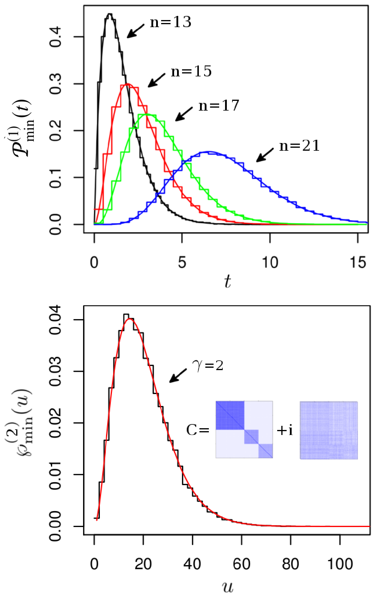
time series ($\beta=1$) of lengths $n=13,15,17,21$. As empirical eigenvalues $\Lambda_{j}$, we chose 0.6, 1.2, 6.7, 9.3, 10.5, 15.5, 17.2, 20.25, 30.1, 35.4. To demonstrate the validity of our results, we compare them with numerical simulations. Using the program R [42], we generate and diagonalize 50,000 correlated random Wishart matrices drawn from the distribution (2). As expected, the agreement is perfect. In contrast to the formulae in Ref. [39], numerical evaluation of Eq. (19) is easily possible even for large matrix dimension $p$.

We now show the existence of a new kind of universality in the correlated Wishart model. In addition to the theoretical interest in this issue, the universal results to be presented now might also be of practical importance when analyzing correlation matrices built from many long time series. We want to zoom into a local scale set by the mean level spacing of the spectral density near the origin. To this end, we consider the limit $n,p\longrightarrow\infty$ in such a way that the “rectangularity” $n-p$ is held fixed. A similar limit, referred to as microscopic, was introduced in Chiral Random Matrix Theory [25, 26], which models statistical aspects of Quantum Chromodynamics. However, in contrast to our case the probability density is fully rotation invariant, corresponding to $\Lambda=\mathbb{1}_{p}$. Here we consider an arbitrary $\Lambda$, and thus have to take into account how the local mean level spacing depends on $\Lambda$. From Refs. [43, 41] it follows that we have to rescale $t$ with $p$, when taking the limit $p\longrightarrow\infty$. Hence we introduce a new variable $u$ by making the ansatz

with a $\Lambda$ dependent constant $\eta$ yet to be determined. We thus we restrict our analysis to the commonly encountered situation in which almost all empirical eigenvalues do not depend on $p$, and only few are proportional to $p$. In the microscopic limit, the gap probability and the distribution of the smallest eigenvalue are defined as

The limit $p\rightarrow\infty$ is non–trivial, because the function $f_{\beta,\bar{n}}(\sigma)$ and the normalization constant depend on $p$. The $p$ dependence of the latter is determined by evaluating Eq. (13) at $t=0$, which shows that $K_{p\times\bar{n}}=(-1)^{\gamma p}\text{det}^{-\gamma}\Lambda~K_{\gamma}$ with $K_{\gamma}$ independent of $p$. Next we investigate how the $p$ fold product of determinants in Eq. (13) behaves on the local scale,

Expanding the logarithm to leading order in $1/p$ shows that we have to choose

to fix the microscopic scale, provided $\eta$ converges to a non zero constant for $p\rightarrow\infty$. The large–$p$ limit of the above expression is then

The factor $(-1)^{\gamma p}\text{det}^{\gamma}\Lambda$ cancels with the $p$ dependent part of $K_{p\times\bar{n}}$. Combining $\det^{p\beta/2}\sigma$ with Eq. (15) and performing a series of integrations by parts leads to

which can be evaluated either by using $\delta$ functions or by proper contour integration. Remarkably, the very same matrix model results on the microscopic scale in the case that all empirical eigenvalues are equal to $1/\eta$, as seen from Eq. (13),

where $\eta$ dropped out on the right–hand side. Thus, we have effectively traced back the problem to the uncorrelated case considered in Refs. [44, 34, 43, 45, 46]. Using the scaling Eq. (22), with $\eta$ given by Eq. (26), the results coincide with the formulae of Ref. [45],

where $L^{(l)}_{ij}(u)=\sqrt{u/4}^{i+j-\kappa^{\prime}}\text{I}_{\kappa^{\prime}+\delta_{i-l,0}-i-j}\left(\sqrt{u}\right)$ and $\text{I}_{\nu}$ is the modified Bessel function of order $\nu$. We also have defined $\kappa^{\prime}=2(\gamma+1)/\beta$ and $\tilde{q}_{ij}=(j-i)$ for $\beta=1$, $\tilde{q}_{ij}=(-1)^{i+1}$ for $\beta=2$. The distribution of the smallest eigenvalue on the microscopic scale is then given by

To illustrate this new universality, we carry out numerical simulations for $\wp^{(2)}_{\footnotesize\text{min}}(u)$ shown in Fig. 1. We generate 30,000 Hermitian Wishart correlation matrices with $p=200$ and $n=202$, for a non-trivial empirical correlation matrix $C$ as indicated in Fig. 1.

In conclusion, we have calculated the gap probability and the distribution of the smallest eigenvalue for the complex and the real correlated Gaussian Wishart ensemble. By numerical evaluation of our results we demonstrated that they are easy to use in applications. We also found a new universality on the microscopic scale. On the conceptual level, our most important result is the discovery of the duality between the $W$ and the $\overline{W}$ matrix models. Actually, there are infinitely many dualities, as there is full freedom in choosing that dimension of the matrices which corresponds to the number of time steps. In turn, each of these models has a dual model in superspace with, in general, different bosonic and fermionic dimensions. Of course, here we chose the simplest duality that led to a model in a superspace which collapses to an ordinary space, because the bosonic dimension is zero. A presentation with further results and more mathematical details will be given elsewhere [38].