A Bayesian changepoint methodology for high dimensional multivariate time series and space-time data: A study of structural change using remotely sensed data.

Chris Strickland Robert Burdett Robert Denham Robert Kohn Kerrie Mengersen Note: c.strickland@unsw.edu.au, University of New South Wales, robert.burdett@qut.edu.au, Queensland University of Technology, robert.denham@qld.gov.au, Queensland Department of Science, Information Technology, Innovation and the Arts, r.kohn@unsw.edu.au, University of New South Wales, kerrie.mengersen@qut.edu.au, Queensland University of Technology

Abstract

A Bayesian approach is developed to analyze change points in multivariate time series and space-time data. The methodology is used to assess the impact of extended inundation on the ecosystem of the Gulf Plains bioregion in northern Australia. The proposed approach can be implemented for dynamic mixture models that have a conditionally Gaussian state space representation. Details are given on how to efficiently implement the algorithm for a general class of multivariate time series and space-time models. This efficient implementation makes it feasible to analyze high dimensional, but of realistic size, space-time data sets because our approach can be appreciably faster, possibly millions of times, than a standard implementation in such cases.

Keywords. conditionally Gaussian, state space model, environmental data, dynamic factor model

1 Introduction

The Gulf Plains bioregion of northern Australia is a large area of tropical savanna on extensive alluvial plains and coastal areas (Thackway and Cresswell,, 1997). The region experiences a monsoonal climate with a winter dry season and a summer wet season, with the wet season typically extending from October to April. A monsoon season from December to March brings significant rainfall, often causing flooding throughout the region. Flooding can be extensive, and floodwaters can remain on pasture for several weeks. In general, the floodplains are resilient ecosystems, adapted to the wet and dry seasons, with grasslands responding rapidly after the wet season. However, periods of extended inundation can have an adverse lasting effect on pasture, resulting in the death of grasses and seed bank.

The summer of 2008/2009 in this region experienced one of the most severe floods on record, with widespread prolonged flooding from January to March (Bureau of Meteorology,, 2009). There was widespread reports of death of grasses, and a lack of recovery the following year. The region is remote with limited infrastructure, so a remotely sensed approach to monitor the extent and the timing of the event is desirable. In this paper, we use the Normalized Difference Vegetation Index (NDVI) from NASA’s Moderate Resolution Imaging Spectroradiometer (MODIS) to determine the timing, effect size and recovery time following an extended flood event. MODIS data is used extensively to identify disturbance from time series data, though this typically uses image difference techniques using only a small number of image dates (Jin and Sader,, 2005; Nielsen,, 2007, e.g.), or uses univariate time series models (Verbesselt et al., 2010a, ; Verbesselt et al., 2010b, , e.g.). The former approach is not suitable as it ignores the time series structure present in the problem, while the latter method ignores the information available through common trends, as well as any spatial correlation present in the data. Unlike these methods the approach presented in this paper, uses all of the data and takes account of both the temporal and spatial correlation structure in the data.

Specifically, we propose a method for analysing data with an unknown number of changepoints that is applicable to high-dimensional multivariate time series and space-time data. The detection of change in time series and space-time data sets is of paramount importance in many areas of statistics, and as a consequence it has been the focus of much recent research; see, for example, Majumdar et al., (2004), Koop and Potter, (2007), Giordani and Kohn, (2008) and Koop and Potter, (2009).

Mixture innovation models, cast in a conditionally Gaussian state space framework, provide an intuitive and flexible approach for modeling non-linear effects, and furthermore they can be used for models that allow for an unknown number of changepoints. The idea behind this approach is to account for change by modeling the state innovation using a mixture distribution. While approximate methods have been developed for this class of models, see for example Harrison and Stephens, (1976) and Smith and West, (1983), it has been the advent of modern simulation methods that has facilitated the development of exact methods. Early methods utilizing Markov chain Monte Carlo (MCMC) include McCulloch and Tsay, (1993) and Carter and Kohn, (1994). A drawback of these approaches is that sampling the auxiliary discrete variables, used to define the mixture on the innovations, is done conditionally on the states. This often results in a poorly mixing MCMC sampler because of the high dependence between the states and the auxiliary discrete variables. For the univariate conditionally Gaussian state space model, Gerlach et al., (2000) propose an algorithm that generates the auxiliary discrete variables in $O(n)$ operations, without conditioning on the states, where $n$ is the sample size. This is an important development because it overcomes the potentially high dependence between the auxiliary discrete variables and the states inherent in the algorithm of Carter and Kohn, (1994).

Our article makes four major methodological contributions to the Bayesian literature. First, the methodology of Gerlach et al., (2000) is extended to multivariate conditionally Gaussian state space models. Second, let $p$ be the dimension of the observation vector in any time period. Then for a fairly general class of $p-$ dimensional state space models, which apply to both multivariate time series and space-time analysis, we show how to sample from the posterior distribution of interest using $O\left(pn\right)$ operations, rather than $O\left(p^{3}n\right)$ operations, in the case of a naive implementation of the algorithm. We show that this results in a increase in the speed that is of practical significance (possibly millions of times faster) for the size of data that is of interest to us. Third, the structure of the prior for the model and the MCMC methodology allows us to average over the model space generated by the common components in, possibly high dimensional, multivariate time series and space-time models. This feature of our approach is very important at a practical level, as well as being theoretically attractive, particularly as the number of common components increase in the specified model. Fourth, we propose a general approach for sampling candidates in the latent state process of our model that is efficient with respect to both computation and simulation. In particular, we show how to draw in order $O(pn)$ operations any parameter that enters the model only through the state transition equation. Here, generating the parameter is done from its conditional distribution with the states integrated out. We believe that each of these contributions is necessary in producing a method, which contains an adequately rich model structure and can be feasibly used to analyze data sets of the size that are of interest to fields such as remote sensing.

The new methodology is used to detect change in the NDVI that is measured from the Moderate Resolution Imaging Spectroradiometer satellite. The space-time data set consists of nearly 18000 spatial locations at 268 time points.

The article is organised as follows. Section 2 describes the conditionally Gaussian multivariate state space model and the new sampling algorithm. Section 3 describes the hierarchical multivariate time series and space-time model, its efficient implementation, a computational comparison of the efficient implementation and a naive implementation and a description of an MCMC algorithm for the model. Section 4 demonstrates the methodology on simulated data. Section 5 utilizes the new methodology to analyze structural change in the NDVI for the Gulf plains bioregion in northern Australia. data. Section 6 summarizes the article. All proofs of the results in the article are in the appendix.

2 Conditionally Gaussian Multivariate State Space Model

The observation vector $\bm{y}_{t}\in\mathbb{R}^{p},$ for $t=1,2,\dots,n,$ for the conditionally Gaussian state space model (CGSSM) is generated by

\bm{y}_{t}=\bm{g}_{t}+\bm{H}_{t}\bm{x}_{t}+\bm{G}_{t}\bm{e}_{t},

(1)

where $\bm{g}_{t}\in\mathbb{R}^{p}$ , $\bm{H}_{t}\in\mathbb{R}^{p\times m}$ and $\bm{G}_{t}\in\mathbb{R}^{p\times p}$ are system matrices and $\bm{e}_{t}\in\mathbb{R}^{p}$ is independently and normally distributed, with mean $\bm{0}\in\mathbb{R}^{p}$ and a covariance $\bm{I}_{p},$ where $\bm{I}_{p}$ denotes an identity matrix of order $p$ . The state vector, $\bm{x}_{t}\in\mathbb{R}^{m},$ for $t=1,2,\dots,n-1,$ is generated by the difference equation

\bm{x}_{t+1}=\bm{h}_{t}+\bm{F}_{t}\bm{x}_{t}+\bm{\Gamma}_{t}\bm{u}_{t},

(2)

with $\bm{h}_{t}\in\mathbb{R}^{m},$ the transition matrix $\bm{F}_{t}\in\mathbb{R}^{m\times m},$ $\bm{\Gamma}_{t}\in\mathbb{R}^{m\times r}$ and the disturbance vector $\bm{u}_{t}\in\mathbb{R}^{r}$ is defined to be serially uncorrelated and normally distributed with a mean $\bm{0}\in\mathbb{R}^{r}$ and a covariance matrix $\bm{I}_{r}$ . The system matrices in (1) and (2) are functions of the unknown parameters $\bm{\omega}\in\mathbb{R}^{l}$ and also depend on a sequence of discrete random variables $\bm{K}_{t}\in\mathbb{R}^{s},$ which can be used to model non-linear effects in an intuitive manner. The state space model is completed by specifying the distribution of the initial state $\bm{x}_{1}$ as

\bm{x}_{1}\sim N\left(\bm{m}_{1},\bm{V}_{1}\right),

(3)

with mean $\bm{m}_{1}\in\mathbb{R}^{m}$ and covariance $\bm{V}_{1}\in\mathbb{R}^{m\times m}$ . For notational convenience throughout, denote $\bm{x}=\left(\bm{x}_{1},\bm{x}_{2},\dots,\bm{x}_{n}\right)$ and $\bm{x}^{s:t}=\left(\bm{x}_{s},\bm{x}_{s+1},\dots,\bm{x}_{t}\right),$ where this convention extends to any vector or matrix.

2.1 Estimation

Algorithm 1 provides a general way of estimating the model described in (1)–(3).

1.

Sample $\bm{K}^{\left(j\right)}$ from $p\left(\bm{K}|\bm{y},\bm{\omega}^{\left(j-1\right)}\right)$
2.

Sample $\bm{x}^{\left(j\right)}$ from $p\left(\bm{x}|\bm{y},\bm{K}^{\left(j\right)},\bm{\omega}^{\left(j-1\right)}\right)$ .
3.

Sample $\bm{\omega}^{\left(j\right)}$ from $p\left(\bm{\omega}|\bm{y},\bm{x}^{\left(j\right)},\bm{K}^{\left(j\right)}\right)$ .

Algorithm 1

Step 3 of Algorithm 1 is model specific. Steps 1 and 2 can be completed using algorithms that are applicable to the general state space model. Specifically, in Step 1, $\bm{K}$ is sampled from $p\left(\bm{K}|\bm{y},\bm{\omega}\right)$ by sampling each $\bm{K}_{t},$ for $t=1,2,\dots,n,$ from $p\left(\bm{K}_{t}|\bm{y},\bm{K}_{s\neq t}\right).$ The algorithm used in this computation is described below. In Step 2, $\bm{x}$ is drawn from $p\left(\bm{x}|\bm{y},\bm{K},\bm{\omega}\right).$ This step, which involves sampling the state from its full conditional posterior distribution, can be achieved using any of the algorithms developed by Carter and Kohn, (1994), Frühwirth-Schnatter, (1994), de Jong and Shephard, (1995), Durbin and Koopman, (2002) or Strickland et al., (2009). Sampling $\bm{K}$ is the most difficult step, and is achieved through a generalization of results presented by Gerlach et al., (2000) who propose an algorithm to efficiently sample $\bm{K},$ for the univariate state space model, i.e. when $\bm{y}_{t}$ is a scalar. Their contribution is to show that $\bm{K}$ can be sampled in $O\left(n\right)$ operations, without needing to condition on the states $\bm{x}.$ The idea builds on the relation

$\displaystyle p\left(\bm{K}_{t}\|\bm{y},\bm{K}_{s\neq t},\bm{\omega}\right)$	$\displaystyle\propto$	$\displaystyle p\left(\bm{y}\|\bm{K},\bm{\omega}\right)\times p\left(\bm{K}_{t}\|\bm{K}_{s\neq t},\bm{\omega}\right)$	(5)
	$\displaystyle\propto$	$\displaystyle p\left(\bm{y}^{t+1:n}\|\bm{y}^{1:t},\bm{K},\bm{\omega}\right)\times p\left(\bm{y}_{t}\|\bm{y}^{1,t-1},\bm{K}^{1:t},\bm{\omega}\right)\times$
		$\displaystyle p\left(\bm{K}_{t}\|\bm{K}_{s\neq t},\bm{\omega}\right),$

where the term $p\left(\bm{K}_{t}|\bm{K}_{s\neq t},\bm{\omega}\right)$ is obtained from the prior, and may depend on unknown parameters, the term $p\left(\bm{y}_{t}|\bm{y}^{1,t-1},\bm{K}^{1:t},\bm{\omega}\right)$ is obtained using one step of the Kalman filter and the term $p\left(\bm{y}^{t+1:n}|\bm{y}^{1:t},\bm{K},\bm{\omega}\right)$ is obtained by one forward step after initially doing a set of backward recursions.

Given Lemmas A.1, A.1.2 and A.1.3 (see the appendix), an algorithm for sampling $\bm{K}$ from $p\left(\bm{K}|\bm{y},\bm{\theta}\right)$ is defined as follows:

1.

Given the current value of $\bm{K},$ for $t=n-1,n-2,\dots,1,$ compute $\bm{\mu}_{t}$ and $\bm{\Omega}_{t}$ using the recursion given in A.1.
2.

For $t=1,2,\dots,n,$
1. (a)
  
  compute $p\left(\bm{y}_{t}|\bm{y}^{1:t-1},\bm{K}^{1:t},\bm{\omega}\right)$ using A.1.2,
2. (b)
  
  compute $p\left(\bm{y}^{t+1:n}|\bm{y}^{1:t},\bm{K},\bm{\omega}\right)$ using A.1.3,
3. (c)
  
  for all values of $\bm{K}_{t}$ compute $p\left(\bm{K}_{t}|\bm{y},\bm{\omega}\right)$ and form a probability mass function and use it to sample $\bm{K}_{t}.$
4. (d)
  
  re-run one step of the Kalman filter, defined in A.1.2, based on the sample $\bm{K}_{t}.$

Algorithm 2 Algorithm to sample

\bm{K}.

3 Hierarchical Time Series and Space-Time Modeling

We consider a general modeling framework that applies to both multivariate time series and space-time analysis. In particular, the observation equation at time $t,$ for $t=1,2,\dots,n,$ for the observations, $\bm{y}_{t}\in\mathbb{R}^{p},$ is

\bm{y}_{t}=\bm{\Theta}\bm{f}_{t}+\bm{\bm{e}}_{t},

(6)

where $\bm{\Theta}\in\mathbb{R}^{p\times k}$ is a matrix of basis functions, which is possibly spatially referenced, $\bm{f}_{t}\in\mathbb{R}^{k}$ is a vector of common components and $\bm{e}_{t}\in\mathbb{R}^{p}$ is a vector of serially uncorrelated, normally distributed disturbances, with diagonal covariance matrices $\bm{\Sigma}_{t}\in\mathbb{R}^{p\times p}$ . The matrix of basis functions, $\bm{\Theta},$ in the case of multivariate time series analysis is typically taken as unknown and the model in (6) is commonly referred to as a dynamic factor model (DFM). In space-time analysis a wide variety of basis functions have been used in its specification, including empirical orthogonal functions EOF, Fourier and wavelet bases, amongst many other methods; see Cressie and Wikle, (2011) for a thorough review. When $\bm{\Theta}$ is unknown, it is assumed to be a function of a vector of parameters, $\bm{\kappa},$ which needs to be estimated. We specify the structure of $\bm{\Theta}$ when applying the model in Sections 4 and 5. Regardless of the specification of the matrix of basis functions, its purpose is the same: to provide a mapping between the high dimensional set of observations and a low dimensional system that aims to capture the dynamic characteristics in the data generating process. This method of dimension reduction is necessary computationally and practically sensible. For example, in remotely sensed data one may expect that observations in woodlands might exhibit a common temporal signature, and data points in grasslands exhibit a different but also common temporal signature. Our models can take advantage of such features present in the data. Typically the common terms, $\bm{f}_{t},$ are sums of a number of components such as trend, regression and autoregressive components. To estimate the model in a state space framework, it is convenient to define $\bm{f}_{t}=\bm{\Phi}\bm{x}_{t},$ where $\bm{\Phi}\in\mathbb{R}^{k\times m}$ is a selection matrix that is used so that the model in (6) can be written in state space form. It follows that,

	$\displaystyle\bm{y}_{t}$	$\displaystyle=$	$\displaystyle\bm{\Theta}\bm{\Phi}\bm{x}_{t}+\bm{e}_{t},$		(7)
	$\displaystyle\bm{x}_{t+1}$	$\displaystyle=$	$\displaystyle\bm{W}_{t}\bm{\beta}+\bm{F}_{t}\bm{x}_{t}+\bm{\Lambda}_{t}\bm{v}_{t},$		(8)

where $\bm{W}_{t}\in\mathbb{R}^{m\times k^{R}}$ is a matrix of regressors, $\bm{\beta}\in\mathbb{R}^{k^{R}}$ is a vector of regression coefficients, $\bm{\Lambda}_{t}\in\mathbb{R}^{m\times r}$ and $\bm{v}_{t}\in\mathbb{R}^{r}$ is a random vector that is normally distributed with a covariance matrix $\bm{I}_{m}$ . It is immediately apparent that (7) and $\left(\ref{eq:state_DFM}\right)$ can be expressed as the CGSSM in (1) and (2), by defining $\bm{H}_{t}=\bm{\Theta}\bm{\Phi},$ $\bm{G}_{t}=\bm{\Sigma}_{t}^{\frac{1}{2}},$ $\bm{h}_{t}=\bm{W}_{t}\bm{\beta}$ and $\bm{\Gamma}_{t}=\bm{\Lambda}_{t}.$ Note that for certain classes of basis functions, it may be necessary to impose identification restrictions on the model.

3.1 The Multiple Change Point Problem

Modeling multiple change points, using a variation of Algorithm 1, is accomplished by defining $\bm{\Lambda}_{t}$ to be a function of $\bm{K}_{t}.$ Specifying a model to handle changepoints in this way is simple and flexible. For example, we can specify each common component to consist of an autoregressive process and a level that allows for shifts in the conditional mean and slope of the process. This is achieved, for $i\in\mathbb{N}^{k},$ where $\mathbb{N}^{k}$ denotes the set $\left\{1,2,\dots,k\right\},$ by defining

f_{i,t}=\psi_{i,t}+\mu_{i,t}+\bm{w}_{t-1}^{T}\bm{\beta}_{i},

(9)

where $\psi_{i,t}$ is an autoregressive cyclical process, $\mu_{i,t}$ is the level, $\bm{w}_{t}\in\mathbb{R}^{k^{r}}$ is a vector of regressors and $\bm{\beta}_{i}\in\mathbb{R}^{k^{r}}$ is a vector of regression coefficients. Specifically, we define $\psi_{i,t}$ as a damped stochastic cycle, such that

\psi_{i,t+1}=\rho_{i}\left(\cos\left(\lambda_{i}\right)\psi_{i,t}+\sin\left(\lambda_{i}\right)\psi_{i,t}^{*}\right)+\sigma_{f,i}\zeta_{i,t},

where $\rho_{i}$ is a persistence parameter, $\lambda_{i}$ is a hyperparameter that defines the period of the cycle, $\psi_{i,t}^{*}$ is an auxiliary variable defined by

\psi_{i,t+1}^{*}=\rho_{i}\left(\cos\left(\lambda_{i}\right)\psi_{i,t}^{*}-\sin\left(\lambda_{i}\right)\psi_{i,t}\right)+\sigma_{f,i}\zeta_{i,t}^{*},

$\sigma_{f,i}$ is a scale parameter and $\zeta_{i,t}$ and $\zeta_{i,t}^{*}$ are standard normal random variables. The stochastic cycle reverts to a standard first order autoregressive process when $\lambda_{i}=0;$ for further details on stochastic cycles, see Harvey, (1989). The cycle is used to capture seasonal effects in the analysis in this paper. The level $\mu_{i,t}$ is modeled as

\displaystyle\mu_{i,t+1}

\displaystyle=\mu_{i,t}+\delta_{i,t}+\sigma_{f,i}K_{i,t}^{\mu}\xi_{i,t},

\displaystyle\delta_{i,t+1}

\displaystyle=\delta_{i,t}+\sigma_{f,i}K_{i,t}^{\delta}\chi_{i,t}

where $\delta_{i,t}$ captures the slope for the $i^{th}$ common component, $K_{i,t}^{\mu}$ is a discrete random variable that is used to accommodate change in the level, $\xi_{i,t}$ and $\chi_{i,t}$ are independent standard normal random variables; $K_{i,t}^{\delta}$ is a discrete random variable that is used to model changes in the slope.

For $i\in\mathbb{N}^{k},$ the prior for $\rho_{i}$ is a beta distribution, $\mathcal{B}\left(\alpha_{\rho},\beta_{\rho}\right)$ , which ensures that $\psi_{t,i}$ is a stationary process, with a positive autocorrelation function. The prior for $\lambda_{i}$ is a stretched beta distribution, $\mathcal{B}^{\left(a,b\right)}\left(\alpha_{\lambda},\beta_{\lambda}\right),$ where $\mathcal{B}^{(a,b)}\left(\alpha_{\lambda},\beta_{\lambda}\right)$ is a beta distribution that has been translated and stretched over the open set $\left(a,b\right)$ , i.e., if $\zeta_{i}\sim\mathcal{B}\left(\alpha_{\lambda},\beta_{\lambda}\right),$ then $\lambda_{i}=a+\zeta_{i}(b-a)$ . Let $\beta_{i,j}$ be the $j^{th}$ element of $\bm{\beta}_{i}.$ Then, the $\beta_{i,j}$ are a priori independent, i.e., $p\left(\bm{\beta}_{i}\right)=p\left(\beta_{i,1}\right)\times p$ $\left(\beta_{i,2}\right)\times\cdots\times p\left(\beta_{i,k^{r}}\right)$ and

p\left(\beta_{i,j}\right)=\left(1-\varpi_{i,j}\right)\delta_{0}\left(\beta_{i,j}\right)+\varpi_{i,j}\mathcal{N}\left(0,\sigma_{\beta}^{2}\right),

where $\varpi_{i,j}\in\left\{0,1\right\}$ is a Bernoulli auxiliary random variable, such that $\varpi_{i.j}\sim\mathcal{B}ern\left(1,p_{\varpi}\right).$ For $i\in\mathbb{N}^{k},$ the prior for $\sigma_{f,i}$ is an inverted gamma distribution, i.e., $\sigma_{f,i}\sim IG\left(\nu_{f\sigma}/2,s_{f\sigma}/2\right),$ where $\nu_{f_{\sigma}}$ is the degrees of freedom parameter and $s_{f\sigma}$ is the scale parameter.

In our article, the discrete random variables for the $i^{th}$ common component, $K_{i,t}^{\mu}\in\left\{0,\eta_{1,i}^{\mu},\eta_{2,i}^{\mu}\right\}$ and $K_{i,t}^{\delta}\in\left\{0,\eta_{1,i}^{\delta},\eta_{2,i}^{\delta}\right\}$ are used to capture changes in the level and slope, respectively. The elements of $\bm{\eta}=\left(\eta_{1,i}^{\mu},\eta_{2,i}^{\mu},\eta_{1,i}^{\delta},\eta_{2,i}^{\delta}\right)$ are assumed independent a priori with prior distributions that are inverted gamma, where for $j\in\left\{1,2\right\},$ $\eta_{j,i}^{\mu}\sim IG\left(\nu_{j}^{\mu}/2,s_{j}^{\mu}/2\right)$ and $\eta_{j}^{\delta}\sim IG\left(\nu_{j}^{\delta}/2,s_{j}^{\delta}/2\right).$ It is assumed that $\bm{K}_{t}=\left\{K_{i,t}^{\mu},K_{i,t}^{\delta}\right\}_{i\in\mathbb{N}^{k}}$ is multinomial, where at each time point only one change point (in either the level or the slope) is allowed for all $i.$ While we can specify a more general prior, we found that this prior works well for the data sets we have analyzed. The multinomial prior distribution for $\bm{K}_{t}$ is defined assuming that we are in the null state, i.e. $K=0|K\in\bm{K}_{t},$ with probability $1-\pi.$ It is further assumed that $\bm{K}_{t}$ takes any other possible values with equal probability.

$K_{1,t}^{\mu}$	0	$\eta_{1,1}^{\mu}$	$\eta_{2,1}^{\mu}$	0	0	0	0	0	0
$K_{2,t}^{\mu}$	0	0	0	$\eta_{1,2}^{\mu}$	$\eta_{2,2}^{\mu}$	0	0	0	0
$K_{1,t}^{\delta}$	0	0	0	0	0	$\eta_{1,1}^{\delta}$	$\eta_{2,1}^{\delta}$	0	0
$K_{2,t}^{\delta}$	0	0	0	0	0	0	0	$\eta_{1,2}^{\delta}$	$\eta_{2,2}^{\delta}$
$p\left(\bm{K}_{t}\right)$	$\left(1-\pi\right)$	$\frac{\pi}{8}$	$\frac{\pi}{8}$	$\frac{\pi}{8}$	$\frac{\pi}{8}$	$\frac{\pi}{8}$	$\frac{\pi}{8}$	$\frac{\pi}{8}$	$\frac{\pi}{8}$

Table 1: Prior distribution for

\bm{K}_{t}

For example, Table 1 illustrates the case for the two component model. The first four rows of the table capture the possible values for $\bm{K}_{t},$ while the bottom row reports the prior probability of being in each state. For example, the second column of the table shows that the probability of being in the null state is $\left(1-\pi\right),$ while the third column states that $K_{1,t}^{\mu}=\eta_{1,1}^{\mu},K_{2,t}^{\mu}=K_{1,t}^{\delta}=K_{2,t}^{\delta}=0,$ with probability $\frac{\pi}{8}.$

The model for the $i^{th}$ common component in (9) nests many models of interest. In particular, as this approach can be used to account for an unknown number of changepoints, it nests every possibility from the case of no changepoints, i.e. $K_{i,t}^{\mu}=K_{i,t}^{\delta}=0$ for all $t$ so that the model for $f_{i}$ is the cycle plus regression component, to the case of a changepoint in either the mean or slope at every observation. This approach, which determines the model as part of the estimation avoids the need to specify a model for each common component and is of increasing practical importance as the number of common components grows. A theoretical attraction of this approach is that it averages over the model space of common factors and the $\bm{K}_{t}$ discrete variables to correctly account for uncertainty in the model.

The hierarchical model of interest, in which the common components are specified according to (9), can be formulated following (7) and (8), by defining $\bm{x}_{t}=\left[\begin{array}[]{cccc}\bm{x}_{1,t}^{T}&\bm{x}_{2,t}^{T}&\cdots&\bm{x}_{k,t}^{T}\end{array}\right]^{T},$ where $\bm{x}_{i,t}=\left[\begin{array}[]{cccc}\tilde{\psi}_{i,t}&\psi_{i,t}^{*}&\mu_{i,t}&\delta_{i,t}\end{array}\right]^{T},$ with $\tilde{\psi}_{i,t}=\psi_{i,t}-\bm{w}_{t-1}\bm{\beta}_{i}$ and $\bm{\Phi}=\text{diag}\left(\bm{\phi}_{1}^{T},\bm{\phi}_{2}^{T},\dots,\bm{\phi}_{k}^{T}\right),$ with $\bm{\phi}_{1}=\bm{\phi}_{2}=\cdots=\bm{\phi}_{k}=\left[\begin{array}[]{cccc}1&0&1&0\end{array}\right].$ Furthermore, the state transition matrix $\bm{F}_{t}=\text{diag}\left(\bm{F}_{1,t},\bm{F}_{2,t},\dots,\bm{F}_{k,t}\right),$ with $\bm{F}_{i,t}$ a $4\times 4$ block diagonal matrix, with $(\bm{F}_{i,t})_{11}=(\bm{F}_{i,t})_{22}=\rho_{i}\cos(\lambda),(\bm{F}_{i,t})_{12}=-(\bm{F}_{i,t})_{21}=\rho_{i}\sin(\lambda)$ and $(\bm{F}_{i,t})_{33}=(\bm{F}_{i,t})_{34}={\bm{F}_{i,t}}_{44}=1$ ; the rest of the elements of $\bm{F}_{i,t}$ are zero. The system matrix $\bm{\Lambda}_{t}=\text{diag}\left(\bm{\Lambda}_{1,t},\bm{\Lambda}_{2,t},\dots,\bm{\Lambda}_{k,t}\right),$ with $\bm{\Lambda}_{i,t}=\text{diag}\left(1,1,K_{1,t}^{\mu},K_{2,t}^{\delta}\right)$ . The regressors are formulated such that for $t=1,2,\dots,n-1,$ $\bm{W}_{t}=\text{diag}\left(\bm{W}_{t,1},\bm{W}_{t,2},\dots,\bm{W}_{t,k}\right),$ where $\bm{W}_{t,i}$ is a $(4\times 2)$ matrix, with $(\bm{W}_{t,i})_{11}=\bm{w}_{t}-\rho_{i}\cos\left(\lambda_{i}\right)\bm{w}_{t-1}$ , $(\bm{W}_{t,i})_{21}=\rho_{i}\sin\left(\lambda_{i}\right)\bm{w}_{t-1}$ , and where the rest of the elements in $\bm{W}_{t,i}=0$ ; $\bm{W}_{0}$ is a $(4\times 2)$ matrix, with $(\bm{W}_{0})_{11}=\omega_{0}$ , $(\bm{W}_{0})_{31}=1$ ; the rest of the elements in $\bm{W}_{0}=0$ . Note that $\bm{\beta}=\left(\bm{\beta}_{1}^{T},\mu_{1,1},\bm{\beta}_{2}^{T},\mu_{2,1},\dots,\bm{\beta}_{k}^{T},\mu_{k,1}\right).$

3.2 Efficient Estimation

Sampling $\bm{K}=\left\{\bm{K}_{t},\,t=1,2,\dots,n\right\}$ for the hierarchical model in (7) and (8) using Algorithm 2 is straightforward but very inefficient, as it involves $O\left(p^{3}n\right)$ operations. The following Lemma (see Appendix A.1 for a proof) shows how to sample $\bm{K}_{t}$ from $p\left(\bm{K}_{t}|\bm{y},\bm{K}_{s\neq t},\bm{\omega}\right)$ far more efficiently.

Lemma 3.2.1.

Suppose that in the hierarchical model in (7) and (8), $\bm{K}$ enters only through the state equation. Then it is possible to sample $\bm{K}$ using $p\left(\bm{K}_{t}|\bm{y},\bm{K}_{s\neq t},\bm{\omega}\right)$ by applying Algorithm 2 to the transformed state space model

\bm{y}_{t}^{L}=\bm{\Psi}\bm{x}_{t}+\bm{e}_{t}^{L},

(10)

where $\bm{y}_{t}^{L}=\left(\bm{\Theta}^{T}\bm{\Sigma}_{t}^{-1}\bm{\Theta}\right)^{-1}\bm{\Theta}^{T}\bm{\Sigma}^{-1}\bm{y}_{t},$ $\bm{e}_{t}\sim\mathcal{N}\left(\bm{0},\bm{\Sigma}_{t}^{L}\right),$ with $\bm{\Sigma}_{t}^{L}=\left(\bm{\Theta}^{T}\bm{\Sigma}_{t}^{-1}\bm{\Theta}\right)^{-1}$ and the state equation remains the same as (8).

The transformation in (10) is motivated by Jungbacker and Koopman, (2008), who suggest using the same transformation in sampling the state, $\bm{x},$ from its full conditional posterior distribution, for the case of the DFM. Jungbacker and Koopman also show how to modify the likelihood to correct for the transformation. The lemma shows that it is unnecessary to modify Lemma 3.2.1 to sample $\bm{K}$ . The computational savings that arise from applying Algorithm 2 are dramatic, if the number of time series, $p,$ is large, which is common in space-time analysis; see for example Strickland et al., (2011), where $p$ is close to one thousand, or perhaps even more dramatically in the analysis in Section 5 where $p$ is close to 18000. Specifically, if Algorithm 2 is implemented on the model that has not be transformed then $O\left(p^{3}n\right)$ operations are required. However, for the $k$ -dimensional state space model in (10) and (8) only $O\left(m^{3}n\right)$ operations are required, where the dimension of the state, $m,$ is typically equal to or slightly larger than $k$ , and $k\ll p.$ As such, the main cost of using the transformed model in (10) typically comes from the computation of the transform, which requires $O\left(pn\right)$ operations.

Corollary 3.1.

Suppose that $\bm{\omega}_{s}$ is a vector of parameters that only appears in the state equation. Then the density

p\left(\bm{\omega}_{s}|\bm{y},\bm{\Theta},\bm{\Sigma},\bm{K}\right)\propto p\left(\bm{y}_{L}|,\bm{K},\bm{\Sigma}_{L}\right)p\left(\bm{\omega}_{s}\right),

(11)

where $p\left(\bm{y}_{L}|,\bm{K},\bm{\Sigma}_{L}\right)=\int p\left(\bm{y}_{L},\bm{x}|\bm{\Sigma}_{L},\bm{K}\right)d\bm{x}$ can be computed by applying the Kalman filter to the lower dimensional SSM in (17) and (8).

Corollary 3.1 is particularly important in constructing efficient sampling schemes for large data sets. Its proof follows from that of Lemma 3.2.1. When using MCMC to analyze large data sets it is important that each component of the MCMC algorithm can be calculated in a computationally efficient manner, and furthermore induce as little correlation as possible in the Markov chain. In some sense the chain is only as strong as its weakest link and thus even if just one component of the MCMC algorithm is inefficient then this can be enough, at least for the large data case, to render the MCMC algorithm impractical. It is straightforward to implement an adaptive RWMH algorithm, based on (11), to sample any of the hyperparameters in the state, where the form of (11) ensures that we are sampling the parameter of interest marginal of $\bm{x}.$ Sampling state hyperparameters, marginal of the state, is shown to significantly improve the simulation efficiency of the resultant estimates in Kim et al., (1998) and Strickland et al., (2009). While we can alternatively compute $p\left(\bm{\omega}_{s}|\bm{y},\bm{\Theta},\bm{\Sigma},\bm{K}\right)\propto p\left(\bm{y}|,\bm{K},\bm{\Sigma}\right)p\left(\bm{\omega}_{s}\right),$ by applying the Kalman filter to the full model in (7) and (8), this would be practically infeasible for large data sets.

3.2.1 Computational Comparison

To illustrate the practical importance of Lemma 3.2.1, (and indirectly illustrate the importance of Corollary 3.1), we compare the time taken with and without applying the results of Lemma 3.2.1. To do so, a simulated data set consisting of 200 temporal observations from the hierarchical model in (7) and (8) is constructed for specific numbers of time series. In each case, we consider a two component model, where the common components are specified with the following dynamics,

\displaystyle f_{i,t+1}

\displaystyle=\mu_{i,t+1}+\rho_{i}\left(f_{i,t}-\mu_{i,t}\right)+\sigma_{f,i}\zeta_{i,t},\hskip 10.00002pt\mu_{i,t+1}=\mu_{i,t}+\sigma_{f,i}K_{i,t}^{\mu}\xi_{i,t}.

(12)

Number of time series	5	10	50	100	500	1000	5000	10000	100000	500000
Ignores Lemma 3.2.1	30	43	515	1407	$27978^{*}$	$149831^{*}$	$12788430^{*}$	$95654412^{*}$	NA	NA
Uses Lemma 4	24	24	24	24	25	25	28	29	68	239
Relative speed up	1.25	1.7	21	59	$1119^{*}$	$5993^{*}$	$456730^{*}$	$3298428^{*}$	NA	NA

Table 2: The table reports the observed or estimated^∗ time (in seconds) running 1000 calls of Algorithm 2, both when Lemma 3.2.1 is employed and when it is not, for different sized data sets. We report the estimated time when it is impractical to run 1000 iterations for a given data set. In this case fewer iterations are used and the timings from the reduced run are used to estimate the time taken for 1000 iterations.

Table 2 summarizes the computational expense of using Algorithm 2, both when Lemma 3.2.1 is used and when it is not. The first row of the table lists the number of time series in the analysis. The second and third rows report the time (note that we report estimated time when it is not practical in all cases to run 1000 iterations, so fewer iterations are used and the timings from the reduced run are used to estimate the time taken for 1000 iterations) in seconds for 1000 calls of Algorithm 2, ignoring Lemma 3.2.1 and taking advantage of Lemma 3.2.1, respectively. The fourth row reports the relative speed up that is achieved when taking advantage of Lemma 3.2.1. All timings are done using a Linux operating system, with a 3.2GHz Intel Core i7 processor, with 24 Gigabytes of RAM. All computation is done using a combination of the Python and Fortran programming languages.

The table shows that the savings that arise from Lemma 3.2.1 are particularly dramatic as the number of time series grows. In fact, it is essential to use Lemma 3.2.1 for any application of large space-time data sets, as the time difference between using and not using the lemma can range from a few minutes, to waiting perhaps a few years.

4 Analysis of Simulated Data

To critically evaluate the methodology, we first analyze a simulated data set, consisting of 400 time series of length 300 observations. A two factor standard DFM is specified where the factors are essentially of the same form as (9). The hyperparameters are set so that $\rho_{1}=0.8,$ $\rho_{2}=0.9$ , $\lambda_{1}=\lambda_{2}=\frac{2\pi}{23},$ $\sigma_{f,1}=\sigma_{f,2}=0.5.$ We set $k^{r}=3$ , where the regressors are simulated from a standard normal distribution. We set the regression coefficients to be the same for each factor and set $\beta_{11}=\beta_{21}=0.8,$ $\beta_{12}=\beta_{22}=0.9$ and $\beta_{31}=\beta_{32}=0.001.$ The structural breaks are deterministically rather than stochastically defined, as this is more sensible for the purpose of validation. The level for the first common factor, $\mu_{t,1},$ is constant except for a deterministic break that is defined at the $200^{th}$ observation. The second common factor, $\mu_{t,2},$ is defined to be constant except for deterministic breaks at the $50^{th},75^{th},100^{th}$ and $150^{th}$ observations. In addition, the second common factor has a break in the slope at the $240^{th}$ observation. For identification purposes it is assumed that $\Theta_{i,i}=1.0$ and for all $j>i$ $\Theta_{j,i}=0.0$ ; see Harvey, (1989) for further details on identification restrictions for DFMs. To specify the prior on $\bm{\Theta},$ let $\bm{\theta}_{i}\in\mathbb{R}^{p-i}$ be a vector formed from the non-deterministic elements in the $i^{h}$ column of $\bm{\Theta}$ . The prior for $\bm{\Theta}$ is $p\left(\bm{\Theta}\right)=p\left(\bm{\theta}_{1}\right)p\left(\bm{\theta}_{2}\right)\dots p\left(\bm{\theta}_{k}\right),$ where

p\left(\bm{\theta}_{i}\right)\sim N\left(\bm{0},\kappa_{i}^{-1}\bm{I}\right),

$\kappa$ is the prior precision, and we assume $\kappa_{i},$ for $i\in\mathbb{N}^{k},$ follows a gamma distribution, such that $\kappa_{i}\sim G\left(\frac{\nu_{\kappa}}{2},\frac{S\kappa}{2}\right).$ Note that, for this prior, conditional on the state, $\bm{x},$ the $p$ equations that make up the measurement equation are independent and consequently it is straightforward to sample $\bm{\Theta}$ and $\bm{\kappa}$ from their respective posterior distributions using standard Bayesian linear regression theory.

4.1 Prior Specification

Parameter	Hyperparameters	mean	Parameter	Hyperparameters	mean
$\left\{\rho_{i}\right\}_{i\in\mathbb{N}^{k}}$	$\alpha_{\rho}=15$ and $\beta_{\rho}=1.5$	0.91	$\left\{\eta_{\delta 2,i}\right\}_{i\in\mathbb{N}^{k}}$	$\nu_{\delta 2}=3$ and $s_{\delta 2}=0.4$	0.5
$\left\{\sigma_{f,i}\right\}_{i\in\mathbb{N}^{k}}$	$\nu_{f\sigma}=10$ and $s_{f\sigma}=0.1$	0.1	$\left\{\lambda_{i}\right\}_{i\in\mathbb{N}^{k}}$	$\alpha_{\lambda}=2,$ $\beta_{\lambda}=2,$ $a=0$ and $b=\frac{4\pi}{23}$	$\frac{2\pi}{23}$
$\left\{\eta_{\mu 1,i}\right\}_{i\in\mathbb{N}^{k}}$	$\nu_{\mu 1}=3$ and $s_{\mu 1}=30$	4.4	$\left\{\sigma_{m,i}\right\}_{i\in\mathbb{N}^{p}}$	$\nu_{m}=10$ and $s_{m}=0.1$	0.1
$\left\{\eta_{\mu 2,i}\right\}_{i\in\mathbb{N}^{k}}$	$\nu_{\mu 2}=3$ and $s_{\mu 2}=300$	13.8	$\left\{\beta_{i,j}\right\}_{i\in\mathbb{N}^{k},j\in\mathbb{N}^{k_{r}}}$	$\sigma_{\beta}=3$	0.0
$\left\{\eta_{\delta 1,i}\right\}_{i\in\mathbb{N}^{k}}$	$\nu_{\delta 1}=3$ and $s_{\delta 1}=0.1$	0.25	$\left\{\varpi_{i,j}\right\}_{i\in\mathbb{N}_{+}^{k},j\in\mathbb{N}^{k_{r}}}$	$p_{\varpi}=0.5$	0.5

Table 3: The table reports the values of the prior hyperparameters.

Table 3 reports the values of the prior hyperparameters used in the analysis as well as the corresponding prior means. The prior mean for $\phi_{i}$ and $\sigma_{i},$ for $i\in\mathbb{N}^{k},$ imply that a priori we assume a fairly high level of persistence and a small signal for each of the common factors. The values of the prior hyperparameters for $\eta_{\mu 1}$ and $\eta_{\mu 2},$ for $i\in\mathbb{N}^{k},$ imply that for each level we allow for breaks of two different sizes. Likewise, the prior values for $\eta_{\delta 1}$ and $\eta_{\delta 2},$ for $i\in\mathbb{N}^{k},$ allows for two different sizes of shifts in the slope. The prior for $\lambda_{i}$ corresponds to a period of 23 observations. This is the typical number of observations in one year of MODIS data. In addition we assume that $\nu_{\kappa}=10$ and $S_{\kappa}=0.01.$ The prior for $\varpi_{i},$ for $i\in\mathbb{N}^{k},$ $j\in\mathbb{N}^{k^{r}}$ implies that a priori that the standard first order autoregressive process and the stochastic cycle are equally probable.

Refer to caption — Figure 1: a) Plots the estimated (solid line) trend for factor 1 against the truth (dashed line). b) Plots the estimated (solid line) for the autoregressive state for factor 1 against the truth (dashed line). c) Plots the estimated (solid line) trend for factor 2 against the truth (dashed line). d) Plots the estimated (solid line) autoregressive state for factor 2, against the truth (dashed line). e) Plots the simulated data set.

Figure 1 shows the marginal posterior mean estimates of the trend and autoregressive component, based on an MCMC analysis, using Algorithm 3, using 5000 iterations, with the first 1000 discarded. Panels a) and b) show the marginal posterior mean estimates of the trend and seasonal component, respectively, for the first common component, where the seasonal component refers to the cycle plus regression components. In particular the solid line represents the marginal posterior mean estimates and the dashed line is represents the truth. The plots show that the estimates closely follow the truth, and importantly captures the timing of the changepoint in the level. The estimates for the second common factor can be seen through Panels c) and d), and show that the timing of the level shifts have been accurately captured and further that the shift in slope seems to be approximately at the correct time. Panel e) plots the simulated data set.

5 Modelling change in NDVI from MODIS imagery

The data set of interest is drawn from an area south of Normanton in Queensland, Australia (141.187^∘ East, 17.843^∘ South), and includes part of the Norman River (Figure 2).

The data consists of a rectangular array of size $128\times 139$ of NDVI from the MODIS satellite. The pixel size is 250 square meters, and the area of interest is approximately 35 by 32 kilometers. This product is available every 16 days, and the data used spans the period from February 2000 to September 2011. In total, 17653 observations over space at 268 time points are analysed, which amounts to a total of 4768256 observations.

Plant growth, and hence NDVI, is primarily related to soil moisture availability, which in turn is related to climatic variables through precipitation and temperature (Wen et al.,, 2012; Wang et al.,, 2003). To model short term variation in NDVI, we used daily climatic data for the region that are extracted from the SILO climate data bank (Jeffrey et al.,, 2001) and averaged over each 16 day interval, or summed in the case of rainfall. Climatic explanatory variables considered are maximum temperature, minimum temperature, rainfall, evaporation, short wave solar radiation for a horizontal surface, atmospheric water vapour pressure, relative humidity at maximum temperature, relative humidity at minimum temperature and reference potential evapotranspiration. Two lags of each regressor are included as explanatory variables in the model and as a consequence the regressors can only really be expected to capture relatively short term seasonal information. We expect any longer term seasonal impact to feed into the trend.

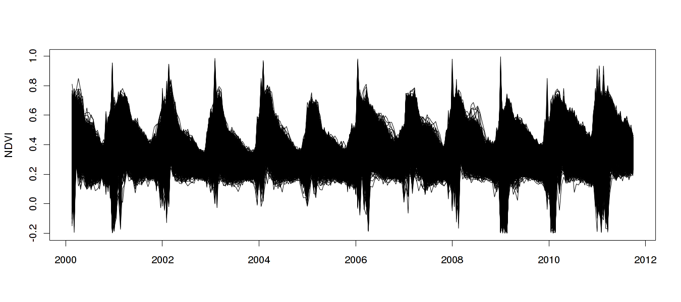
Figure 3 is a time series plot of NDVI for the data set of interest. The plot shows that the data is seasonal with complex dynamics, but without any clear evidence of structural breaks. For the analysis, we use an EOF basis for $\bm{\Theta},$ where $k$ is set so that the $k^{th}$ component explains at least one percent of the variation in the data. The specifications of the priors remain the same as for the analysis of simulated data, and is thus described in Table 3.

Parameter	Mean	Std	IF	Parameter	Mean	Std	IF
$\rho_{1}$	0.95	0.12	5.8	$\lambda_{3}$	0.25	0.03	7.81
$\rho_{2}$	0.64	0.07	7.08	$\lambda_{3}$	0.26	0.03	8.98
$\rho_{3}$	0.68	0.06	6.31	$\sigma_{f,1}$	0.04	0.001	7.25
$\rho_{4}$	0.58	0.08	7.31	$\sigma_{f,2}$	0.02	0.001	8.81
$\lambda_{1}$	0.26	0.02	6.78	$\sigma_{f,3}$	0.022	0.001	6.67
$\lambda_{2}$	0.26	0.03	8.4	$\sigma_{f,4}$	0.03	0.001	6.7

Table 4: The table reports the marginal posterior mean (Mean), marginal posterior standard deviation (Std) and the Inefficiency factor (IF), for each of the specified parameters.

The MCMC analysis using Algorithm 3 is run for 5000 iterations, with the first one thousand iterations are discarded as burnin. Table 4 reports the estimated output for some of the parameters from the MCMC analysis of the MODIS data set. It is clear that for each factor there is a moderate to high level of persistence in the stochastic cycle and for each case the estimated period of the cycle is close to a year, which can be expected. Note that for a period of one year we expect $\lambda=0.26.$ From the inefficiency factors it is evident that the MCMC estimates are extremely efficient, and in fact for all, of the nearly 18000 parameters, are smaller than nine; see Chib and Greenberg, (1996) for further details on inefficiency factors.

Figure 4 plots the trend, seasonal component and the spatial structure in the data, implied by the EOF bases, respectively, for each of the four components. The trend is the marginal posterior mean estimate of $\mu_{i,t},$ for $t=1,2,\dots,n,$ and can be interpreted as the longer term trend in the data. The seasonal component is the marginal posterior mean estimate of $\psi_{i,t}+\bm{w}_{t-1}\bm{\beta}_{i}$ for $t=2,3,\dots,n$ and for $t=1$ is $\bm{w}_{0}\bm{\beta}_{i}.$ The image plots highlight where each particular component has most impact. Essentially the lighter the area the more influence the particular trend has over the data of the corresponding region. Visual inspection of the image plot for the first component, (A), reveals that the corresponding common component in the data is least influential where the water feature is present. For this region, examination of the trend, suggests that NDVI was initially decreasing, but has recovered in more recent years. A moderate El Niño in 2002/2003 resulted in well below average rainfall in this area, and the impact on vegetation is clear in the trend. La Niña events in 2007/2008 and again in 2008/2009 produced above average rainfall, and, as shown in the trend, resulted in a general increase in vegetation in the region. From the image plot we can see that the second component, (B), is most influential in areas close to the river and its tributaries. Structural change is clearly present in the trend for this component. In particular, the trend suggests a substantial drop in NDVI in 2009, corresponding to a known period of prolonged inundation in the region. While periodic inundation is common in much of the lower lying areas in the region, the floods in 2008/2009 were unusual in that areas were under water for a much longer period. Visual interpretation of the trend suggests that for this region the level of NDVI does not immediately recover to previous levels, adding weight to the theory that the prolonged period of inundation caused long term damage to the vegetation. The third and fourth components are less interesting. The calculation of the EOF bases suggest that they account for far less variation in the data. Arguably, component three, (C), seems to have most influence in the outer tributaries of the water system. The trend suggests an overall increase of NDVI over time for this region, at least above and beyond that of what is explained by components (A) and (B). The fourth component, (D), arguably shows an increase in NDVI over time as well, up until the point of the inundation, where it drops and flattens off. It is also interesting to note that the seasonal pattern is most regular away from the river and tributaries. This is not unexpected as this region is less susceptible to flooding, in which case we can expect a more uniform response to climatic factors.

6 Conclusions

This article introduces a Bayesian methodology for the detection of structural change in multivariate time series and space-time data. Remotely sensed data is used in the analysis of the Gulf Plains bioregion, where, using the proposed methodology, we found evidence of structural change in a region that had been inundated for an extended period of time. Areas most affected by the 2009 flood have not recovered to pre-flood levels in over two and a half years.

This research was partially supported by Australian Research Council linkage grant, LP100100565. The research of Robert Kohn was partially supported by Australian Research Council grant DP066706. All computation was undertaken using the Python van Rossum, (1995) and Fortran programming languages. We made use of the libraries, NumPy, SciPy Oliphant, (2007), PyMCMC Strickland et al., (2012) and PySSM
(https://bitbucket.org/christophermarkstrickland/pyssm). The code also makes heavy use of BLAS and Lapack though ATLAS
(http://math-atlas.sourceforge.net/) and F2PY Peterson, (2009).

Appendix A Appendix

A.1 Lemmas and Proofs

Lemma A.1.1.

For $t=1,2,\dots,n,$ the conditional density $\bm{y}^{t+1:n}$ given $\bm{x}_{t}$ and $\bm{K}$ , ignoring terms that are not a function of $\bm{x}_{t}$ or $\bm{K}$ , may be expressed as

p\left(\bm{y}^{t+1:n}|\bm{x}_{t},\bm{K},\bm{\omega}\right)\propto\exp\left\{-\frac{1}{2}\left(\bm{x}_{t}^{T}\bm{\Omega}_{t}\bm{x}_{t}-2\bm{\mu}_{t}^{T}\bm{x}_{t}\right)\right\},

(13)

where the terms $\bm{\Omega}_{t}$ and $\bm{\mu}_{t}$ can be computed through a set of backward recursions. Specifically, the backward recursions used in sampling $\bm{K}$ for the multivariate conditional state space model in (1) and (2) are computed by first initializing $\bm{\mu}_{n}=\bm{0}$ and $\bm{\Omega}_{n}=\bm{0},$ where $\bm{\mu}_{t}\in\mathbb{R}^{m}$ and $\bm{\Omega}_{t}\in\mathbb{R}^{m\times m},$ then for $t=n-1,n-2,\dots,1,$ first computing

$\displaystyle\bm{J}_{t+1}$	$\displaystyle=\bm{H}_{t+1}\bm{\Gamma}_{t}$	$\displaystyle\bm{R}_{t}$	$\displaystyle=\bm{J}_{t+1}\bm{J}_{t+1}^{T}+\bm{G}_{t}\bm{G}_{t}^{T}$
$\displaystyle\bm{L}_{t+1}$	$\displaystyle=\bm{\Omega}_{t+1}\bm{C}_{t+1}\bm{D}_{t+1}^{-1}\bm{C}_{t+1}^{T}$	$\displaystyle\bm{N}_{t+1}$	$\displaystyle=\bm{\Gamma}_{t+1}\left(\bm{I}-\bm{J}_{t+1}^{T}\bm{R}_{t+1}^{-1}\bm{J}_{t+1}\right)\bm{\Gamma}_{t+1}^{T}$
$\displaystyle\bm{C}_{t+1}$	$\displaystyle=\bm{N}_{t+1}^{\frac{1}{2}}$	$\displaystyle\bm{D}_{t+1}$	$\displaystyle=\bm{I}+\bm{C}_{t+1}^{T}\bm{\Omega}_{t+1}\bm{C}_{t+1}$	(14)
$\displaystyle\bm{B}_{t+1}$	$\displaystyle=\bm{R}_{t+1}^{-1}\bm{J}_{t+1}\bm{\Gamma}_{t+1}^{T}$	$\displaystyle\bm{E}_{t+1}$	$\displaystyle=\bm{I}-\bm{B}_{t+1}^{T}\bm{H}_{t+1}$
$\displaystyle\bm{K}_{t}$	$\displaystyle=\bm{I}-\bm{L}_{t}$	$\displaystyle\bm{M}_{t+1}$	$\displaystyle=\bm{R}_{t+1}^{-1}\bm{H}_{t+1}\bm{F}_{t}$
$\displaystyle\bm{S}_{t+1}$	$\displaystyle=\bm{K}_{t+1}\bm{\Omega}_{t+1}$	$\displaystyle\bm{q}_{t+1}$	$\displaystyle=\bm{\Omega}_{t+1}\left(\bm{E}_{t+1}\bm{h}_{t}+\bm{B}_{t+1}^{T}\left(\bm{y}_{t+1}-\bm{g}_{t+1}\right)\right)$
$\displaystyle\bm{A}_{t+1}$	$\displaystyle=\bm{E}_{t+1}\bm{F}_{t}$

where $\bm{J}_{t},\bm{L}_{t},\bm{R}_{t}\in\mathbb{R}^{p\times p},$ $\bm{B}_{t},\bm{M}_{t}\in\mathbb{R}^{p\times m},$ $\bm{N}_{t},\bm{C}_{t},\bm{D}_{t},\bm{E}_{t},\bm{A}_{t},\bm{S}_{t}\in\mathbb{R}^{m\times m}$ and $\bm{q}_{t}\in\mathbb{R}^{m}$ and then computing

	$\displaystyle\bm{\Omega}_{t}$	$\displaystyle=\bm{A}{}_{t+1}^{T}\bm{\Omega}_{t+1}\bm{S}_{t+1}+\bm{M}_{t+1}^{T}\bm{H}_{t+1}\bm{F}_{t}$
	$\displaystyle\bm{\mu}_{t}$	$\displaystyle=\bm{A}{}_{t+1}\bm{K}_{t+1}\left(\bm{\mu}_{t+1}-\bm{q}_{t+1}\right)+\bm{M}_{t+1}^{T}\left(\bm{y}_{t+1}-\bm{g}_{t+1}-\bm{H}_{t+1}\bm{h}_{t+1}\right).$		(15)

Proof.

To derive the set of equations in (14) and (15), first define $\bm{r}_{t+1},$ such that

\displaystyle\bm{\varepsilon}_{t+1}

\displaystyle=

\displaystyle\bm{y}_{t+1}-\mathbb{E}\left(\bm{y}_{t+1}|\bm{x}_{t},\bm{K}^{1,t+1}\right)=\bm{y}_{t+1}-\bm{g}_{t+1}-\bm{H}_{t+1}\left(\bm{h}_{t}+\bm{F}_{t}\bm{x}_{t}\right)=\bm{J}_{t+1}\bm{u}_{t}+\bm{G}_{t+1}\bm{u}_{t+1},

where $\bm{J}_{t+1}=\bm{H}_{t+1}\bm{\Gamma}_{t},$ and define $\bm{R}_{t+1}$ as $\bm{R}_{t+1}=var\left(\bm{y}_{t+1}|\bm{x}_{t},\bm{K}^{1,t+1}\right)=\bm{J}_{t+1}\bm{J}_{t+1}^{T}+\bm{G}_{t+1}\bm{G}_{t+1}^{T}.$

Noting that $\mathbb{E}\left(\bm{x}_{t+1}|\bm{x}_{t},\bm{y}_{t+1},\bm{K}^{1,t+1}\right)=\mathbb{E}\left(\bm{x}_{t+1}|\bm{x}_{t},\bm{\varepsilon}_{t+1},\bm{K}^{1,t+1}\right),$ $Cov\left(\bm{\varepsilon}_{t},\bm{x}_{t}\right)=\bm{0}$ and $\mathbb{E}\left(\bm{\varepsilon}_{t}\right)=\bm{0},$ it then follows

$\displaystyle\mathbb{E}\left(\bm{x}_{t+1}\|\bm{x}_{t},\bm{\varepsilon}_{t+1},\bm{K}\right)$	$\displaystyle=$	$\displaystyle\mathbb{E}\left(\bm{x}_{t+1}\|\bm{x}_{t},\bm{K}\right)+Cov\left(\bm{x}_{t+1}\bm{\eta}_{t+1}\|\bm{K}\right)\bm{R}_{t+1}^{-1}\bm{\eta}_{t+1}$
	$\displaystyle=$	$\displaystyle\bm{E}_{t+1}\bm{h}_{t}-\bm{B}_{t+1}^{T}\bm{g}_{t+1}+\bm{B}_{t+1}^{T}\bm{y}_{t+1}+\bm{E}_{t+1}\bm{F}_{t}\bm{x}_{t}$
	$\displaystyle=$	$\displaystyle\bm{a}_{t+1}+\bm{A}_{t+1}\bm{x}_{t}+\bm{B}_{t+1}\bm{y}_{t+1},$

where

	$\displaystyle\bm{E}_{t+1}$	$\displaystyle=$	$\displaystyle\bm{I}-\bm{B}_{t+1}^{T}\bm{H}_{t+1},\text{ }\bm{a}_{t+1}=\bm{E}_{t+1}\bm{h}_{t}-\bm{B}_{t+1}^{T}\bm{g}_{t+1}$
	$\displaystyle\bm{A}_{t+1}$	$\displaystyle=$	$\displaystyle\bm{E}_{t+1}\bm{F}_{t},\text{ }\bm{B}_{t+1}=\bm{R}_{t+1}^{-1}\bm{J}_{t+1}\bm{\Gamma}_{t}^{T}.$

Let $\bm{N}_{t+1}=var\left(\bm{x}_{t+1}|\bm{x}_{t},\bm{y}_{t+1},\bm{K}\right).$ Then $\bm{N}_{t+1}=\bm{\Gamma}_{t}\left(I-\bm{J}_{t+1}^{T}\bm{R}_{t+1}^{-1}\bm{J}_{t+1}\right)\bm{\Gamma}_{t}^{T}.$ Let $\bm{C}_{t+1}=\bm{N}_{t+1}^{1/2},$ where $\bm{N}_{t+1}^{1/2}$ is defined as $\bm{N}_{t+1}=\left(\bm{N}_{t+1}^{1/2}\right)\left(\bm{N}_{t+1}^{1/2}\right)^{T}.$ Then we can express $\bm{x}_{t+1}$ as

$\bm{x}_{t+1}=\bm{a}_{t+1}+\bm{A}_{t+1}\bm{x}_{t}+\bm{B}_{t+1}^{T}\bm{y}_{t+1}+\bm{C}_{t+1}\bm{z}_{t+1},$ where $\bm{z}_{t+1}\sim N\left(\bm{0},\bm{I}\right)$ and is independent of $\bm{x}_{t}$ and $\bm{y}_{t+1}$ (conditional on $\bm{K}).$ We can factor

$p\left(\bm{y}^{t+1,n}|\bm{x}_{t},\bm{K}\right)=p\left(\bm{y}^{t+2,n}|\bm{y}_{t+1},\bm{x}_{t},\bm{K}\right)\times p\left(\bm{y}_{t+1}|\bm{x}_{j},\bm{K}\right)$ ,

where $p\left(\bm{y}^{t+2,n}|\bm{y}_{t+1},\bm{x}_{t},\bm{K}\right)=\int p\left(\bm{y}^{t+2,n}|\bm{x}_{t+1},\bm{K}\right)p\left(\bm{z}_{t+1}|\bm{K}\right)d\bm{z}_{t+1}.$ Using the form of (13) it follows that

$\displaystyle p\left(\bm{y}^{t+2,n}\|\bm{y}_{t+1},\bm{x}_{t},\bm{K}\right)$	$\displaystyle=$	$\displaystyle\int p\left(\bm{y}^{t+2,n}\|\bm{x}_{t+1},\bm{K}\right)p\left(\bm{z}_{t+1}\|\bm{K}\right)d\bm{z}_{t+1}$
	$\displaystyle\propto$	$\displaystyle\exp\left\{-\frac{1}{2}\left[\bm{x}_{t}^{T}\left(\bm{A}_{t+1}^{T}\bm{\Omega}_{t+1}\bm{A}_{t+1}-\bm{A}_{t+1}^{T}\bm{\Omega}_{t+1}\bm{C}_{t+1}\bm{D}_{t+1}^{-1}\bm{C}_{t+1}^{T}\bm{\Omega}_{t+1}\bm{A}_{t+1}\right)\bm{x}_{j}\right.\right.$
	$\displaystyle-$	$\displaystyle\left.\left.2\bm{x}_{j}^{T}\bm{A}_{t+1}^{T}\left(\left(\bm{I}-\bm{\Omega}_{t+1}\bm{C}_{t+1}\bm{D}_{t+1}^{-1}\bm{C}_{t+1}^{T}\right)\mbox{$\left(\bm{\mu}_{t+1}-\bm{\Omega}_{t+1}\left(\bm{a}_{t+1}+\bm{B}_{t+1}^{T}\bm{y}_{t+1}\right)\right)$}\right)\right]\right\},$

where $\bm{D}_{t+1}=\bm{I}+\bm{C}_{t+1}^{T}\bm{\Omega}_{t+1}\bm{C}_{t+1}.$ Combining $p\left(\bm{y}^{t+2,n}|\bm{y}_{t+1},\bm{x}_{t},\bm{K}\right)$ with $p\left(\bm{y}^{t+2,n}|\bm{y}_{t+1},\bm{x}_{t},\bm{K}\right)$ , where

p\left(\bm{y}_{t+1}|\bm{x}_{t},\bm{K}\right)\propto\exp\left\{-\frac{1}{2}\left(\bm{y}_{t}-\bm{g}_{t+1}-\bm{H}_{t+1}\left(\bm{h}_{t}+\bm{F}_{t}\bm{x}_{t}\right)\right)\bm{R}^{-1}\left(\bm{y}_{t}-\bm{g}_{t+1}-\bm{H}_{t+1}\left(\bm{h}_{t}+\bm{F}_{t}\bm{x}_{t}\right)\right)^{T}\right\},

and completing the square then it follows that

$\bm{\Omega}_{t}=\bm{A}{}_{t+1}^{T}\bm{\Omega}_{t+1}\bm{S}_{t+1}+\bm{M}_{t+1}^{T}\bm{H}_{t+1}\bm{F}_{t},$ with $\bm{S}_{t+1}=\bm{K}_{t+1}\bm{\Omega}_{t+1},$ where $\bm{K}_{t+1}=\bm{I}-\bm{L}_{t},$ $\bm{L}_{t}=\bm{\Omega}_{t+1}\bm{C}_{t+1}\bm{D}_{t+1}^{-1}\bm{C}_{t+1}^{T}$ and $\bm{M}_{t+1}=\bm{R}_{t+1}^{-1}\bm{H}_{t+1}\bm{F}_{t+1}.$ Further,

\bm{\mu}_{t}=\bm{A}{}_{t+1}\bm{K}_{t+1}\left(\bm{\mu}_{t+1}-\bm{q}_{t+1}\right)+\bm{M}_{t+1}^{T}\left(\bm{y}_{t+1}-\bm{g}_{t+1}-\bm{H}_{t+1}\bm{h}_{t+1}\right).

∎

Lemma A.1.2.

The conditional density of $\bm{y}_{t}$ given $\bm{y}^{1:t-1}$ and $\bm{K}^{1:t}$ may be expressed as

p\left(\bm{y}_{t}|\bm{y}^{1:t-1},\bm{K}^{1:t},\bm{\theta}\right)\propto\left|\bm{R}_{t}\right|^{-\frac{1}{2}}\exp\left\{-\frac{1}{2}\left(\bm{\eta}_{t}^{T}\bm{R}_{t}^{-1}\bm{\eta}_{t}\right)\right\},

where the quantities $\bm{\eta}_{t}\in\mathbb{R}^{p}$ and $\bm{R}_{t}\in\mathbb{R}^{p\times p}$ are calculated using the following recursion, with $\bm{m}_{1}$ and $\bm{V}_{1}$ obtained from the prior in (3),

$\displaystyle\bm{r}_{t}$	$\displaystyle=\bm{y}_{t}-\bm{g}_{t}-\bm{H}_{t}\bm{m}_{t}$	$\displaystyle\bm{m}_{t}$	$\displaystyle=\bm{h}_{t-1}+\bm{F}_{t-1}\bm{m}_{t-1\|t-1}$
$\displaystyle\bm{R}_{t}$	$\displaystyle=\bm{H}_{t}\bm{V}_{t}\bm{H}_{t}^{T}+\bm{G}_{t}\bm{G}_{t}^{T}$	$\displaystyle\bm{J}_{t}$	$\displaystyle=\bm{R}_{t}^{-1}\bm{H}_{t}\bm{V}_{t}$
$\displaystyle\bm{V}_{t}$	$\displaystyle=\bm{F}_{t-1}\bm{V}_{t-1\|t-1}\bm{F}_{t-1}^{T}+\bm{\Gamma}_{t-1}\bm{\Gamma}_{t-1}^{T}$	$\displaystyle\bm{V}_{t\|t}$	$\displaystyle=\bm{V}_{t}-\bm{J}_{t}^{T}\bm{R}_{t}\bm{J}_{t}$
$\displaystyle\bm{m}_{t\|t}$	$\displaystyle=\bm{m}_{t}+\bm{J}_{t}^{T}\bm{\eta}_{t}.$

Proof.

It is straightforward to verify that $\bm{r}_{t}=\bm{y}_{t}-\mathbb{E}\left(\bm{y}_{t}|\bm{y}^{1,t-1},\bm{K}^{1,t}\right)=\bm{g}_{t}+\bm{H}_{t}\bm{m}_{t},$ where $\bm{m}_{t}=\mathbb{E}\left(\bm{x}_{t}|\bm{y}^{1,t-1},\bm{K}^{1,t}\right)=\bm{f}_{t-1}+\bm{F}_{t-1}\bm{m}_{t-1|t-1}.$ Furthermore, $\bm{R}_{t}=Cov\left(\bm{\eta}_{t}|\bm{y}^{1,t-1},\bm{K}\right)=\mathbb{E}\left(\bm{\eta}_{t}\bm{\eta}_{t}^{T}|\bm{y}^{1,t-1},\bm{K}\right)=\bm{H}_{t}\bm{V}_{t}\bm{H}_{t}^{T}+\bm{G}_{t}\bm{G}_{t}^{T},$ where $\bm{V}_{t}=Cov\left(\bm{x}_{t}|\bm{y}^{1,t-1},\bm{K}^{1,t}\right)=\bm{F}_{t-1}\bm{V}_{t-1|t-1}\bm{F}_{t-1}^{T}+\bm{\Gamma}_{t-1}\bm{\Gamma}_{t-1}^{T}.$

	$\displaystyle\bm{m}_{t\|t}$	$\displaystyle=$	$\displaystyle\mathbb{E}\left(\bm{x}_{t}\|\bm{y}^{1,t},\bm{K}\right)=\mathbb{E}\left(\bm{x}_{t}\|\bm{y}^{1,t-1},\bm{K}\right)+Cov\left(\bm{x}_{t},\bm{\eta}_{t}\|\bm{y}^{1,t-1},\bm{K}\right)Cov\left(\bm{\eta}_{t}\|\bm{y}^{1,t-1},\bm{K}\right)^{-1}\bm{\eta}_{t}$
		$\displaystyle=$	$\displaystyle\bm{m}_{t-1}+\bm{J}_{t}^{T}\bm{\eta}_{t},$

where $\bm{J}_{t}=\bm{R}_{t}^{-1}\bm{H}_{t}\bm{V}_{t|t},$ with $\bm{V}_{t|t}=\bm{V}_{t}-\bm{J}_{t}^{T}\bm{R}_{t}\bm{J}_{t}$ and

$\displaystyle\bm{V}_{t\|t}$	$\displaystyle=$	$\displaystyle Cov\left(\bm{x}_{t}\|\bm{y}^{1,t},\bm{K}\right)$
	$\displaystyle=$	$\displaystyle Cov\left(\bm{x}_{t}\|\bm{y}^{1,t-1},\bm{K}\right)-Cov\left(\bm{x}_{t},\bm{\eta}_{t}\|\bm{y}^{1,t-1},\bm{K}\right)Cov\left(\bm{\eta}_{t}\|\bm{y}^{1,t-1},\bm{K}\right)^{-1}Cov\left(\bm{x}_{t},\bm{\eta}_{t}\|\bm{y}^{1,t-1},\bm{K}\right)^{T}$
	$\displaystyle=$	$\displaystyle\bm{V}_{t}-\bm{J}_{t}^{T}\bm{R}_{t}\bm{J}_{t}.$

∎

Lemma A.1.3.

Factorize $\bm{V}_{t|t}$ as $\bm{T}\bm{T}^{T}$ and write $\bm{x}_{t}=\bm{m}_{t}+\bm{T}_{t}\bm{\xi}_{t},$ where $\bm{\xi}_{t}\sim\mathcal{N}\left(\bm{0},\bm{I}\right)$ and is independent of $\bm{y}^{1:t}.$ It then follows that the conditional density for $\bm{y}_{t}$ given $\bm{y}^{1:t-1}$ and $\bm{K}^{1:t}$ is

	$\displaystyle p\left(\bm{y}^{t+1:n}\|\bm{y}^{1:t},\bm{K}\right)$	$\displaystyle=$	$\displaystyle\int p\left(\bm{y}^{t+1:n}\|\bm{x}_{t}\right)p\left(\bm{\xi}_{t}\|\bm{K}^{1:t}\right)$		(16)
		$\displaystyle\propto$	$\displaystyle\left\|\bm{Z}_{t}\right\|^{-1/2}\exp\left\{-\frac{1}{2}\left[\bm{m}_{t}^{T}\left(\bm{\Omega}_{t}\bm{m}_{t}-2\bm{\mu}_{t}\right)-\bm{o}_{t}^{T}\bm{T}_{t}\bm{Z}_{t}^{-1}\bm{T}_{t}^{T}\bm{o}_{t}\right]\right\},$		(16)

where $\bm{o}_{t}=\bm{\mu}_{t}-\bm{\Omega}_{t}\bm{m}_{t}$ and $\bm{Z}_{t}=\bm{T}_{t}^{T}\bm{\Omega}_{t}\bm{T}+\bm{I}$ . The proof of this Lemma follows directly from Gerlach et al., (2000).

Proof of Lemma 3.2.1

Proof.

To prove Lemma 3.2.1 holds we need to show that $p\left(\bm{K}_{t}|\bm{y}^{L},\bm{K}_{t\neq s},\bm{\Sigma}^{L},\bm{\omega}\right)\propto p\left(\bm{K}_{t}|\bm{y},\bm{K}_{t\neq s},\bm{\Theta},\bm{\Sigma},\bm{\omega}\right),$ when $\bm{K}_{t}$ only enters through the state equation. We begin by expressing (6) as

\tilde{\bm{y}}_{t}=\tilde{\bm{\Theta}}\bm{f}_{t}+\tilde{\bm{e}}_{t};\,\,\,\tilde{\bm{e}}_{t}\sim N\left(\bm{0},\bm{I}_{p}\right),

(17)

where $\bm{\tilde{y}}_{t}=\bm{\Sigma}^{1/2}\bm{y}_{t}$ and $\tilde{\bm{\Theta}}=\bm{\Sigma}^{1/2}\bm{\Theta}.$ Next, we decompose $\tilde{\bm{\Theta},}$ using the QR decomposition, such that $\bm{\tilde{y}}_{t}=\left[\bm{Q}_{1},\bm{Q}_{2}\right]\left[\begin{array}[]{c}\bm{R}\\ \bm{0}\end{array}\right]\bm{f}_{t}+\tilde{\bm{e}}_{t},$ where $\bm{Q}_{1}\in\mathbb{R}^{p\times k}$ and $\bm{Q}_{2}\in\mathbb{R}^{k\times\left(p-k\right)}$ have orthogonal columns. It follows that $\left[\begin{array}[]{c}\bm{Q}_{1}^{T}\\ \bm{Q}_{2}^{T}\end{array}\right]\tilde{y}_{t}=\left[\begin{array}[]{c}\bm{R}\\ \bm{0}\end{array}\right]\bm{f}_{t}+\tilde{\bm{e}}_{t}.$ If we define $\left[\begin{array}[]{c}\bm{z}_{1}\\ \bm{z}_{2}\end{array}\right]=\left[\begin{array}[]{c}\bm{Q}_{1}^{T}\\ \bm{Q}_{2}^{T}\end{array}\right]\tilde{\bm{y}}_{t}$ then $\left[\begin{array}[]{c}\bm{z}_{1}\\ \bm{z}_{2}\end{array}\right]=\left[\begin{array}[]{c}\bm{R}f_{t}+\bm{e}_{1,t}\\ \bm{e}_{2,t}\end{array}\right].$ Clearly,

p\left(\bm{K}_{t}|\bm{K}_{s\neq t}|\bm{z}_{1},\bm{\omega},\bm{\Sigma}\right)\propto p\left(\bm{K}_{t}|\bm{K}_{s\neq t}|\bm{z}_{1},\bm{z}_{2},\bm{\omega},\bm{\Sigma}\right).

(18)

because $\bm{K}_{t}$ only enters through the state transition equation. Note that for the transformed measurement equation in (17)

	$\displaystyle\bm{y}_{t}^{L}$	$\displaystyle=$	$\displaystyle\left(\tilde{\bm{\Theta}}^{T}\tilde{\bm{\Theta}}\right)^{-1}\tilde{\bm{\Theta}}^{T}\tilde{\bm{y}}_{t}=\left(\bm{R}^{T}\bm{R}\right)^{-1}\left[\begin{array}[]{cc}\bm{R}^{T}&\bm{0}\end{array}\right]\left[\begin{array}[]{c}\bm{z}_{1,t}\\ \bm{z}_{2,t}\end{array}\right]$		(23)
		$\displaystyle=$	$\displaystyle\left(\bm{R}^{T}\bm{R}\right)^{-1}\bm{R}^{T}\bm{z}_{1,t}.$		(23)

Lemma 3.2.1 follows from (18) and (23).

∎

A.2 MCMC Sampling Scheme

1.

Sample $\bm{K}^{\left(j\right)}$ from $p\left(\bm{K},|\bm{y},\bm{\beta}^{\left(j-1\right)}\mbox{,}\bm{\Theta}^{\left(j-1\right)},\bm{\phi}^{(j-1)},\bm{\sigma}_{f}^{(j-1)},\bm{\lambda}^{\left(j-1\right)},\bm{\Sigma}^{\left(j-1\right)},\bm{\eta}^{\left(j-1\right)},\bm{\varpi}^{\left(j-1\right)}\right),$ where $\bm{\phi}=\left(\phi_{1},\phi_{2},\dots,\phi_{k}\right)$ , $\bm{\sigma}_{f}=\left(\sigma_{f,1},\sigma_{f,2},\dots,\sigma_{f,k}\right),$ $\bm{\lambda}=\left(\lambda_{1},\lambda_{2},\dots,\lambda_{k}\right)$ and $\bm{\varpi}=\left(\varpi_{1},\varpi_{2},\dots,\varpi_{k}\right).$
2.

Sample $\bm{x}^{\left(j\right)}$ and $\bm{\beta}^{\left(j\right)},$ jointly from $p\left(\bm{x},\bm{\beta}|\bm{y},\bm{K}^{\left(j\right)}\mbox{,}\bm{\Theta}^{\left(j-1\right)},\bm{\phi}^{(j-1)},\bm{\sigma}_{f}^{(j-1)},\bm{\lambda}^{\left(j-1\right)},\bm{\Sigma}^{\left(j-1\right)},\bm{\eta}^{\left(j-1\right)},\bm{\varpi}^{\left(j-1\right)}\right)$
3.

Sample $\bm{\eta}^{\left(j\right)}$ from $p\left(\bm{\eta}|\bm{x}^{\left(j\right)},\bm{K}^{\left(j\right)},\bm{\beta}^{\left(j\right)},\bm{\phi}^{(j-1)},\bm{\sigma}_{f}^{(j-1)},\bm{\lambda}^{\left(j-1\right)},\bm{\varpi}^{\left(j-1\right)}\right)$ .
4.

Sample $\bm{\phi}^{\left(j\right)}$ from $p\left(\bm{\phi}|\bm{y},\bm{K}^{\left(j\right)},\bm{\Theta}^{\left(j-1\right)},\bm{\beta}^{\left(j\right)},\bm{\sigma}_{f}^{(j-1)},\bm{\Sigma}^{\left(j-1\right)},\bm{\eta}^{\left(j\right)}\right)$ .
5.

Sample $\bm{\sigma}_{f}^{\left(j\right)}$ from $p\left(\bm{\phi}|\bm{y},\bm{K}^{\left(j\right)},\bm{\Theta}^{\left(j-1\right)},\bm{\beta}^{\left(j\right)},\bm{\phi}^{(j)},\bm{\lambda}^{\left(j-1\right)},\Sigma^{\left(j-1\right)},\bm{\eta}^{\left(j\right)}\right)$ .
6.

Sample $\bm{\lambda}^{\left(j\right)}$ from $p\left(\bm{\lambda}|\bm{y},\bm{K}^{\left(j\right)},\bm{\beta}^{\left(j\right)},\bm{\phi}^{\left(j\right)},\bm{\eta}^{\left(j\right)},\bm{\sigma}_{f}^{\left(j\right)}\right).$
7.

Sample $\bm{\varpi}^{\left(j\right)}$ from $p\left(\bm{\varpi}|x^{\left(j\right)},\bm{K}^{\left(j\right)},\bm{\lambda}^{\left(j\right)},\bm{\phi}^{\left(j\right)},\bm{\eta}^{\left(j\right)},\bm{\sigma}_{f}^{\left(j\right)}\right).$
8.

Sample $\bm{\Theta}^{\left(j\right)},\bm{\kappa}$ from $p\left(\bm{\Theta}|\bm{y},\bm{x}^{\left(j\right)},\bm{\Sigma}^{\left(j\right)},\bm{\kappa}^{\left(j-1\right)}\right)$ .
9.

Sample $\bm{\Sigma}^{\left(j\right)}$ from $p\left(\bm{\Sigma}|\bm{y},\bm{x}^{\left(j\right)},\bm{\Theta}^{\left(j\right)}\right).$

Algorithm 3

Algorithm 3 defines the MCMC algorithm for the hierarchical multivariate time series and space-time model that is being considered. Step 1 is unchanged from Algorithm 1. Step 2 only requires a small modification from Step 2 of Algorithm 1. In particular, the algorithm to sample $\bm{x}$ is augmented to now sample $\bm{x},$ jointly with $\bm{\beta}$ ; see de Jong and Shephard, (1995) for details on the modifications required to efficiently jointly sample $\bm{x}$ and $\bm{\beta}.$ The remaining steps are specific to the hierarchical model of interest. Step 3 is carried out by sampling each element of $\bm{\eta}$ from its posterior distribution, which are all inverted gamma distributions. In Steps 4, 5 and 6 each element of $\bm{\phi},$ $\bm{\sigma}_{f}$ and $\bm{\lambda}$ is sampled individually using adaptive random walk Metropolis Hastings algorithms; see Garthwaite et al., (2010) for further details. The sampling is done marginally of the state, $\bm{x},$ by taking advantage of Corollary 3.1. In Step 7, we can take advantage of the standard form of the posterior, and sample each element of $\bm{\varpi}$ which has a closed form solution. In particular, for each element of $\bm{\varpi}$ , the posterior distribution is a Bernoulli distribution. In Step 8, sampling $\bm{\Theta}$ and $\bm{\kappa},$ in the case that $\bm{\Theta}$ is unknown, depends on its specification so details are given in the relevant application sections. Step 9 is straightforward as the diagonal elements in $\bm{\Sigma}$ are conditionally independent with inverted gamma posterior distributions.

References

Bureau of Meteorology, (2009) Bureau of Meteorology (2009). Gulf rivers floods January and February 2009. Technical report, Australian Government Bureau of Meteorology.
Carter and Kohn, (1994) Carter, C. and Kohn, R. (1994). On Gibbs sampling for state space models. Biometrika, 81:541–553.
Chib and Greenberg, (1996) Chib, S. and Greenberg, E. (1996). Markov chain Monte Carlo simulation methods in Econometrics. Econometric Theory, 12:409–431.
Cressie and Wikle, (2011) Cressie, N. and Wikle, C. K. (2011). Statistics for Spatio-Temporal Data. Wiley & Sons.
de Jong and Shephard, (1995) de Jong, P. and Shephard, N. (1995). The simulation smoother for time series models. Biometrika, 82:339–350.
Durbin and Koopman, (2002) Durbin, J. and Koopman, S. J. (2002). A simple and efficient simulation smoother for time series models. Biometrika, 81:603–616.
Frühwirth-Schnatter, (1994) Frühwirth-Schnatter, S. (1994). Data augmentation and dynamic linear models. Journal of Time Series Analysis, 15:183–202.
Garthwaite et al., (2010) Garthwaite, P. H., Fan, Y., and Scisson, S. A. (2010). Adaptive optimal scaling of Metropolis-Hastings algorithms using the Robbins-Monroe process. Technical report, University of New South Wales.
Gerlach et al., (2000) Gerlach, R., Carter, C., and Kohn, R. (2000). Efficient Bayesian inference for dynamic mixture models. Journal of the American Statistical Association, 95(451):819–828.
Giordani and Kohn, (2008) Giordani, P. and Kohn, R. (2008). Efficient Bayesian inference for multiple change-point and mixture innovation models. Journal of Business and Economic Statistics, 26:66–77.
Harrison and Stephens, (1976) Harrison, P. J. and Stephens, C. (1976). Bayesian forecasting. Journal of the Royal Statistical Society, Series B, 38:205–247.
Harvey, (1989) Harvey, A. C. (1989). Forecasting structural time series and the Kalman filter. Cambridge University Press, Cambridge, UK.
Jeffrey et al., (2001) Jeffrey, S. J., Carter, J. O., Moodie, K. M., and Beswick, A. R. (2001). Using spatial interpolation to construct a comprehensive archive of Australian climate data. Environmental Modelling and Software, 16(4):309–330.
Jin and Sader, (2005) Jin, S. and Sader, S. A. (2005). MODIS time-series imagery for forest disturbance detection and quantification of patch size effects. Remote Sensing of Environment, 99(4):462 – 470.
Jungbacker and Koopman, (2008) Jungbacker, B. and Koopman, S. J. (2008). Likelihood-based analysis for dynamic factor models. Technical report, Tinbergen Institute.
Kim et al., (1998) Kim, S., Shephard, N., and Chib, S. (1998). Stochastic volatility: Likelihood inference and comparison with ARCH models. Review of Economic Studies, 65(3):361–393.
Koop and Potter, (2007) Koop, G. and Potter, S. (2007). Estimation and forecasting in models with multiple breaks. Review of Economic Studies, 74:763–789.
Koop and Potter, (2009) Koop, G. and Potter, S. (2009). Prior elicitation in multiple change-point models. International Economic Review, 50:751–772.
Majumdar et al., (2004) Majumdar, A., Gelfand, A. E., and Banerjee, S. (2004). Spatiotemporal change-point modelling. Journal of Statistical Planning and Inference, 130:149–166.
McCulloch and Tsay, (1993) McCulloch, J. H. and Tsay, R. S. (1993). Bayesian inference and prediction for mean and variance shifts in autoregressive time series. Journal of the American Statistical Association, 88:968–978.
Nielsen, (2007) Nielsen, A. (2007). The regularized iteratively reweighted mad method for change detection in multi- and hyperspectral data. IEEE Transaction on Image Processing, 16:463–478.
Oliphant, (2007) Oliphant, T. E. (2007). Python for scientific computing. Computing in Science and Engineering, 9:10–20.
Peterson, (2009) Peterson, P. (2009). F2PY: a tool for connecting Fortran and Python programs. International Journal of Computational Science and Engineering, 4:296–605.
Smith and West, (1983) Smith, A. F. M. and West, M. (1983). Monitoring renal transplants: an application of the multiprocess Kalman filter. Biometrics, 39:867–878.
Strickland et al., (2012) Strickland, C., Alston, C., Denham, R., and Mengersen, K. (2012). PyMCMC : a Python package for Bayesian estimation using Markov chain Monte Carlo. In Alston, C., Mengersen, K., and Pettitt, T., editors, Case studies in Bayesian statistical modelling and analysis. Wiley and Sons.
Strickland et al., (2011) Strickland, C. M., Simpson, D. P., Turner, I., Denham, R. J., and Mengersen, K. L. (2011). Fast Bayesian analysis of spatial dynamic factor models. Journal of the Royal Statistical Society: Series C (Applied Statistics), 1:109–124.
Strickland et al., (2009) Strickland, C. M., Turner, I., Denham, R. J., and Mengersen, K. L. (2009). Efficient Bayesian estimation of multivariate state space models. Computational statistics and Data Analysis, 12:4116–4125.
Thackway and Cresswell, (1997) Thackway, R. and Cresswell, I. (1997). A bioregional framework for planning the national system of protected areas in australia. Natural Areas Journal, 17(3):241–247.
van Rossum, (1995) van Rossum, G. (1995). Python tutorial, technical report cs-r9526. Technical report, Centrum voor Wiskunde en Informatica (CWI), Amsterdam.
(30) Verbesselt, J., Hyndman, R., Newnham, G., and Culvenor, D. (2010a). Detecting trend and seasonal changes in satellite image time series. Remote Sensing of Environment, 114:106–115.
(31) Verbesselt, J., Hyndman, R., Zeileis, A., and Culvenor, D. (2010b). Phenological change detection while accounting for abrupt and gradual trends in satellite image time series. Remote Sensing of Environment, 114:2970–2980.
Wang et al., (2003) Wang, J., Rich, P., and Price, K. (2003). Temporal responses of NDVI to precipitation and temperature in the central great plains, USA. International Journal of Remote Sensing, 24(11):2345–2364.
Wen et al., (2012) Wen, L., Yang, X., and Saintilan, N. (2012). Local climate determines the NDVI-based primary productivity and flooding creates heterogeneity in semi-arid floodplain ecosystem. Ecological Modelling, 242:116 – 126.

$\displaystyle p\left(\bm{K}_{t}\|\bm{y},\bm{K}_{s\neq t},\bm{\omega}\right)$	$\displaystyle\propto$	$\displaystyle p\left(\bm{y}\|\bm{K},\bm{\omega}\right)\times p\left(\bm{K}_{t}\|\bm{K}_{s\neq t},\bm{\omega}\right)$	(5)
	$\displaystyle\propto$	$\displaystyle p\left(\bm{y}^{t+1:n}\|\bm{y}^{1:t},\bm{K},\bm{\omega}\right)\times p\left(\bm{y}_{t}\|\bm{y}^{1,t-1},\bm{K}^{1:t},\bm{\omega}\right)\times$
		$\displaystyle p\left(\bm{K}_{t}\|\bm{K}_{s\neq t},\bm{\omega}\right),$