Model Reduction With MapReduce-enabled Tall and Skinny Singular Value Decomposition
Abstract
We present a method for computing reduced-order models of parameterized partial differential equation solutions. The key analytical tool is the singular value expansion of the parameterized solution, which we approximate with a singular value decomposition of a parameter snapshot matrix. To evaluate the reduced-order model at a new parameter, we interpolate a subset of the right singular vectors to generate the reduced-order model’s coefficients. We employ a novel method to select this subset that uses the parameter gradient of the right singular vectors to split the terms in the expansion yielding a mean prediction and a prediction covariance—similar to a Gaussian process approximation. The covariance serves as a confidence measure for the reduce order model.
We demonstrate the efficacy of the reduced-order model using a parameter study of heat transfer in random media. The high-fidelity simulations produce more than 4TB of data; we compute the singular value decomposition and evaluate the reduced-order model using scalable MapReduce/Hadoop implementations. We compare the accuracy of our method with a scalar response surface on a set of temperature profile measurements and find that our model better captures sharp, local features in the parameter space.
keywords
model reduction, simulation informatics, MapReduce, Hadoop, tall and skinny SVD1 Introduction & motivation
High-fidelity simulations of partial differential equations are typically too expensive for design optimization and uncertainty quantification, where many independent runs are necessary. Cheaper reduced-order models (ROMs) that approximate the map from simulation inputs to quantities of interest may replace expensive simulations to enable such parameter studies. These ROMs are constructed with a relatively small set of high-fidelity runs chosen to cover a range of input parameter values. Each evaluation of the ROM is a linear combination of basis functions derived from the outputs of the high-fidelity runs; ROM constructions differ in their choice of basis functions and method for computing the coefficients of the linear combination. Projection-based methods project the residual of the governing equations (i.e., a Galerkin projection) to create a relatively small system of equations for the coefficients; see the recent preprint [4] for a survey of projection-based techniques. Alternatively, one may derive a closely related optimization problem to compute the coefficients [9, 10, 14]. These two formulations can provide a measure of confidence along with the ROM. However, they are often difficult to implement in existing solvers since they need access to the equation’s operators or residual.
To bypass the implementation difficulties, one may use response surfaces—e.g., collocation [3, 32] or Gaussian process regression [29]—which are essentially interpolation methods applied to the high-fidelity outputs. They do not need access to the differential operators or residuals and are therefore relatively easy to implement. However, measures of confidence are more difficult to formulate and compute. Several works have explored using interpolation instead of projection or optimization to compute the ROM coefficients. This approach is justified when the governing equations are unknown or only a set of PDE solutions are available [24]. It is also useful when nonlinearities in the governing equations prohibit a theoretically sound Galerkin projection [1, 2]. For these reasons, it has been applied to several problems in aerospace engineering [8, 22, 17, 27].
In this paper, we extend these ideas by equipping an interpolation-based ROM with a novel parameter-dependent confidence measure. We first view the ROM from the perspective of the singular value expansion (SVE) of the parameterized PDE solution, where the left singular functions depend on space and time, and the right singular functions depend on the input parameters. We approximate these functions with the components of a singular value decomposition (SVD) of a tall, dense matrix of solutions computed at a set of input parameter values, i.e., parameter snapshots. Many reduced basis methods use the left singular vectors of the snapshot matrix for the ROM basis, where each snapshot represents a spatially varying solution. In contrast, each column of our snapshot matrix contains the full spatio-temporal solution for a given parameter. We have observed interesting behavior in the right singular vectors in several applications: as the index of the singular vector increases, its components—when viewed as evaluations of a parameter-dependent function—become more oscillatory. This is consistent with the common use of the phrase “higher order modes” to describe the singular vectors with large indices. More importantly, the rate that the singular vectors become oscillatory depends on the parameter. In particular, the singular vectors become oscillatory faster in regions of the parameter space where the PDE solution changes rapidly with small parameter perturbations.
We exploit this observation to devise a heuristic for choosing the subset of the left singular vectors comprising ROM; instead of selecting all left singular vectors whose corresponding singular value is above a chosen threshold, we examine the gradients of the right singular vectors at the parameter value where we wish to evaluate the ROM. After some critical index, the right singular vectors are too irregular to safely interpolate. For each ROM evaluation, the right singular vectors are divided into two categories: (i) those that are sufficiently smooth for interpolation, and (ii) those that oscillate too rapidly. The first category identifies the left singular vectors used in the ROM, and the coefficients are computed with interpolation. The remaining left singular vectors are used to compute a measure of confidence similar to the prediction variance in Gaussian process regression. The number of left singular vectors in each category may be different for different ROM evaluations depending on the irregularity of the right singular vectors at the interpolation point; we explore this in the numerical examples. The heuristics we employ to categorize the right singular vectors are based on the work of Hansen in the context of ill-posed inverse problems [19]. We describe the ROM methodology in Section 2.
In Section 4, we demonstrate the ROM and its confidence measure with a parameter study of heat transfer in random media. A brick is heated on one side, and we measure how much heat transfers to the opposite side given the parameterized thermal conductivity of the material. The high-fidelity simulations use Sandia National Laboratories’ finite element production code Aria [26] on its capacity cluster with a mesh containing 4.2M elements. The study uses 8192 simulations, which produce approximately 4 terabytes of data. We study the effectiveness of the reduced-order model and compare its predictions with a response surface on two relevant scalar quantities of interest computed from the full temperature distribution.
Given the data-intensive computing requirements of this and similar applications, we have chosen to implement the ROM in the popular Hadoop distribution [12] of MapReduce [15]. By expressing each step of the ROM construction in the MapReduce framework, we take advantage of its built-in parallelism and fault tolerance. MapReduce’s scalability enables us to compute the SVD of a snapshot matrix with 64 columns and roughly five billion rows—approximately 2.3 terabytes of data—without the custom hard disk I/O that would be necessary to use standard parallel routines such as Scalapack [7]. The algorithm we use for the SVD in MapReduce is based on the communication-avoiding QR decomposition [16] as described in our previous work [13]. We present the implementation of the ROM in Section 3.
2 A reduced-order modeling approach
Let be the solution of a partial differential equation (PDE), where are the space and time coordinates (three spatial dimensions and a temporal dimension), and is an input parameter. We restrict our attention to models with a single scalar parameter to keep the presentation simple. The ROM employs both interpolation and approximations of derivatives in the parameter space . While these operations are possible with more than one parameter, challenges arise in higher dimensions—e.g., the choice of interpolation nodes and the accuracy of derivatives—that we will avoid. If one is willing to address the difficulties of interpolation and approximating derivatives in multiple dimensions, then our approach can be extended.
The interpretation of as the solution of a PDE is important for two reasons. First, the solution of many PDE models can be shown to be a smooth function of both the space/time variables and the parameter, and we restrict our attention to sufficiently smooth solutions. Second, computational tools will compute at all values of given an input . In other words, we cannot evaluate at a specific without evaluating it for every . We will not discuss refinement of the ROM—i.e., which parameter values to run a new set of high-fidelity runs to best improve an initial ROM—but our heuristic offers a natural criterion for such a selection. We assume that computing for a particular is computationally expensive. We want to use the outputs from a few expensive computations at a chosen set of input parameters to approximate at some other in a manner that is less computationally expensive than solving the differential equation.
We assume that is continuous and square-integrable (). In practice, the techniques we use will perform better if is smooth, e.g., admits continuous derivatives up to some order. Since is continuous, it admits a uniformly convergent series representation known as the singular value expansion (SVE); see [18] for more details on the SVE:
| (1) |
The singular functions and are continuous and orthonormal,
| (2) |
The singular values are positive and ordered in decreasing order,
| (3) |
Hansen discusses methods for approximating the factors of the SVE using the singular value decomposition. We will employ his construction [18, Section 5], which ultimately uses point evaluations of the function to construct a matrix suited for the SVD.
Let with be the points of a discretization of the spatio-temporal domain. A run of the PDE solver produces an approximate solution at these points in the domain for a given input . We assume that the spatio-temporal discretization is sufficient to produce an accurate approximation of the PDE solution for all values of ; in practice, such an assumption should be verified. Let with be a set of input parameters where the approximate PDE solution will be computed; we call these the training runs. The number is the budget of simulations, and we expect that for most cases. In other words, we assume that the number of nodes in the spatio-temporal discretization is much larger than the budget of simulations.
From these approximate solutions, we construct the tall, dense matrix
| (4) |
Next we compute the thin SVD,
| (5) |
where, following [18], we treat and
| (6) |
In other words, we treat the entries of the left and right singular vectors as evaluations of the singular functions at the points and , respectively.
2.1 Oscillations in the singular vectors
We will leverage the work of Hansen [20, 19] on computational methods for linear, ill-posed inverse problems to develop the heuristics for the ROM. He observed that, for a broad class of integral equation kernels found in practice, the singular functions become more oscillatory (i.e., cross zero more frequently) as the index increases. Rigorous proofs of this observation are available for some special cases. However, it is easy to construct kernels whose singular functions do not behave this way. For example, take a kernel whose singular functions become more oscillatory with increasing and shuffle the singular functions. Such counterexamples offer evidence that a general statement is difficult to formulate.
We have observed similar phenomena for functions coming from parameterized partial differential equations. This observation is corroborated by many studies in coherent structures based on the closely related proper orthogonal decomposition [23]. Additionally, we have observed that these oscillations may not increase uniformly over the parameter domain. In particular, the rate of increasing oscillations may be greater in regions of the parameter space where has large parameter gradients; we provide two illustrative examples below.
The components of the singular vectors inherit the observed oscillating behavior of the singular functions. In particular, the oscillations increase as the index increases, and they increase more rapidly in regions corresponding to large differences in the elements of the data matrix . These rapid oscillations manifest as an increase with in the magnitude of the difference between entries of the singular vectors corresponding to evaluations of the singular functions that are nearby in parameter space. For example, the difference between and with neighboring will be greater than the difference between and . (Note that when the model contains more than one parameter, the notion of neighboring becomes more complicated.) However, since there is finite resolution in the parameter space, there is typically some after which the discretization is insufficient to represent the oscillations, and this pattern breaks down. The phenomenon is similar to approximating a sequence of sine waves with increasing frequency using the same grid. We formalize this notion in the following assumption.
Assumption 1.
Let be a closed interval with a discretization , where , and let be defined as in (6). There is an such that the sequence of difference magnitudes between neighboring right singular vector entries will increase for from 1 to , i.e.,
| (7) |
For , the relationship becomes unpredictable due to the finite resolution in the parameter space .
Note our restriction to a single parameter and a uniform discretization of the parameter space. These restrictions can be relaxed with appropriate discretizations of a multivariate space. We will use Assumption 1 to justify a heuristic that distinguishes between singular functions that can be resolved and those that cannot given the discretization.
Next we give two concrete examples of the observed behavior in the right singular vectors. The first is a steady state advection-diffusion type boundary value problem,
| (8) |
with homogeneous boundary conditions. The solution is given by
| (9) |
The parameter represents the ratio of diffusion to advection. Figure 1 shows the results the SVD approximation to the SVE factors for a overresolved model (1999 points in the discretization of the parameter space) and an underresolved model (15 points in the parameter space). Observe how the first seven singular functions scaled by their respective singular values become oscillatory at different rates in different regions of the parameter space. In particular, the singular functions oscillate more rapidly in regions of the parameter space corresponding to more advection. Also note how the underresolved approximations deviate from the overresolved approximations in regions of high oscillations.

The second example is another second order boundary value problem with spatially varying coefficients,
| (10) |
with homogeneous boundary condtions, and
| (11) |
The solution is
| (12) |
which is plotted in the top left of Figure 2. Outside the domain, has a singularity at , which causes to grow rapidly along the line near the boundary . This local feature of the solution results in more rapid oscillations of the singular functions near the boundary . The first seven singular functions, scaled by the singular values, are plotted in Figure 2. The rapid oscillations near the parameter boundary are clearly visible. In those same figures, we plot the components of the corresponding singular vectors, scaled by the singular values, for a data matrix with columns computed at eleven equally spaced parameter values in the interval . Notice how the components of the singular vectors deviate from the singular functions as increases, particularly in the regions of rapid oscillations.

In the next sections, we will exploit the observation of non-uniformly increasing oscillations in the right singular vectors to devise a heuristic for the ROM.
2.2 Constructing the reduced-order model
Recall that the goal is to approximate for some input that was not used to compute a training run. We can use the existence of the SVE to justify the following approach. Since we treat the components of the right singular vectors as evaluations of the singular functions , we can interpolate between the singular vector components to approximate the singular functions at new values of . More precisely, define
| (13) |
where is an interpolation operator that takes a value of and the components of the singular vector as arguments. The form of the interpolant may depend on the selection of the points . For example, if these points are the Chebyshev points or the nodes of a Gaussian quadrature rule, then high order global polynomial interpolation is possible. If the points are uniformly spaced, then one may use piecewise polynomials or radial basis functions.
Unfortunately, the increasingly oscillatory character of the functions as increases combined with the fixed discretization causes concern for any chosen interpolation procedure as approaches . In other words, the smoothness of decreases as increases, which diminishes confidence in the interpolation accuracy. Therefore, we seek to divide the right singular vectors into two groups: those that are smooth enough to accurately interpolate and those that are not. Specifically, we seek an with such that for we have confidence in the accuracy of the interpolant . We treat the remaining interpolations with as unpredictable, and we model them with a random variable. We will discuss the choice of in the next section.
Given , we model the PDE output at the space-time coordinate for the new parameter value as
| (14) |
where are uncorrelated random variables with mean zero and variance one; these represent the uncertainty in the interpolation procedure for increasingly oscillatory functions. Under this construction, the vector of values is a random vector with mean and covariance,
| (15) | ||||
The reduced-order model we propose is the mean of this random vector,
| (16) |
The diagonal components of the covariance matrix provide a measure of confidence for the reduced-order model at each similar to the predication variance of a Gaussian process regression model [29].
Next we show the reduced-order model is equivalent to applying the interpolation procedure independently to the rows of a low rank approximation of the matrix . To set up the notation, partition
| (17) |
where , , and contain columns. Then
| (18) | ||||
Then we have the following proposition.
Proposition 1.
If from (13) is a linear operation, then
| (19) | ||||
Proof.
For a function with evaluations the linear interpolation can be written
| (20) |
for some set of weights . Then,
| (21) | ||||
as required. The covariance expression is easily proved using the linear algebra notation. Define the matrix . Then by the orthogonality of the columns of ,
| (22) |
as required. ∎
2.3 Choosing
We must still choose that determines the split between smooth and non-smooth singular vectors. We will exploit the observation of the oscillating singular vectors from Section 2.1 and make use of Assumption 1. We define the following variation metric,
| (23) |
By Assumption 1, is an increasing function of up to some . Loosely, if is too large, then we have entered the range of where interpolations of are not to be trusted. We will quantify this with a threshold . Given , we choose to be the largest such that .
To determine the appropriate threshold , we use a set of PDE evaluations with for testing, where is not in the training set (i.e., for any or ). We choose a set of candidate thresholds . For each testing models and each candidate threshold, we compute the relative error
| (24) |
where . These errors can be visualized, and the final threshold is chosen so that the error in the testing set is relatively small.
We demonstrate this process using the boundary value problem from (10). The training models consist of solutions computed at eleven equally spaced values of the parameter in the range . We compute a test model at the midpoint of each interval , where was used to compute the training models. The range of the variation metric from (23) for these testing sites is roughly 0.1 to 42.8. We choose 20 candidate thresholds in this range and compute the error in the reduced-order model at the testing sites (see (24)) for each candidate threshold. These errors are displayed in Figure 2.3. We want to choose the split such that the ROM uses the fewest left singular vectors with the maximal accuracy; using fewer singular vectors reduces the computational work and produces a simpler model. The errors in Figure 2.3 show that the reduced-order model is as accurate as possible for each testing site after the fourth candidate threshold, which is roughly . For this threshold, Table 2.3 displays the split between the right singular vectors that admit an accurate interpolant and those that are modeled with a random variable for each of the testing sites. Notice that the number of smooth right singular vectors is smaller for testing sites near the boundary of the parameter domain, which is precisely what we would have expected.
figureThe log of the relative error in the mean prediction of the ROM as a function of and . (Colors are visible in the electronic version.)
| 0.0545 | 4 | 0.0006 |
| 0.1435 | 5 | 0.0007 |
| 0.2325 | 6 | 0.0008 |
| 0.3215 | 6 | 0.0010 |
| 0.4105 | 5 | 0.0013 |
| 0.4995 | 6 | 0.0017 |
| 0.5885 | 4 | 0.0023 |
| 0.6775 | 5 | 0.0034 |
| 0.7665 | 3 | 0.0059 |
| 0.8555 | 2 | 0.0129 |
tableThe split and the corresponding ROM error for and different values of .
We can compare the splitting strategy based on with a standard truncation strategy based on the magnitudes of the singular values of . The mean of the random vector (16) is equivalent to interpolating a truncated SVD approximation of the data matrix , as shown in Proposition 1. However, the magnitudes of the singular values provide no insight into the uncertainty in the interpolation procedure. Our splitting strategy chooses a different truncation for the mean (16) for each based on the capability of the interpolation procedure to accurately approximate the right singular functions at the point . The singular values that are not in the mean contribute to the covariance-based confidence measure from (15). A global truncation based on the singular values would create the same prediction variance for every , and it would always be on the order of the largest truncated singular value. In other words, it provides no information on how the confidence in the prediction changes as varies.
3 Implementation in Hadoop
Constructing the ROM for highly resolved simulations (i.e., large ) requires significant data processing. We have implemented the construction in the MapReduce framework, which enables us to take advantage of Hadoop for large-scale distributed data processing. To construct the reduced-order model, the outputs from the high-fidelity simulations are sent to and stored in the Hadoop cluster. Our implementation then proceeds in three steps:
- 1.
Create the tall-and-skinny matrix from the simulation data.
- 2.
Compute the singular value decomposition of .
- 3.
Generate the coefficients of the reduced-order model and evaluate solutions from the ROM.
In what follows, we give a very brief overview of the MapReduce framework, and then we describe each step of the implementation in Hadoop.
3.1 MapReduce/Hadoop
Google devised MapReduce because of the frustration programmers experienced as they constantly juggled the complexity of developing distributed, fault-tolerant data computational algorithms [15]. Early data-intensive computing at Google was a complex mix of ad hoc scripts. Their solution was the MapReduce computation model: a simple, general interface for a common template behind their data analysis tasks that hides the details of the parallel implementations from the programmer. Due to its generality, the MapReduce computation model has also been an effective paradigm for parallelizing tasks on GPUs [21], multi-core systems [30], and traditional HPC clusters [28].
The MapReduce model consists of two elements inspired by functional programming: a map operation to transform the input into a key/value pair and a reduce operation to process information with the same key. The user provides both functions, which cannot have any side effects. A MapReduce implementation executes the map function on the entire dataset in parallel; see Figure 3. A canonical MapReduce dataset is a terabyte-sized text file split into individual lines. In this case, each map function receives only a few thousand lines from the enormous file, which it processes and sends via shuffle to the appropriate reduce function. The shuffle operation groups map outputs by the key, and the reduce function processes all outputs with the same key—e.g., counting the number of times a word appears in a large collection of documents.
Google’s implementation of MapReduce is proprietary. An alternative, open source implementation named Hadoop has become the industry standard for large-scale data processing. More information on Hadoop can be found at the Cloudera website [31]. The Hadoop Distributed File System (HDFS) is a fault-tolerant, replicated, block file system designed to run using inexpensive, consumer grade hard disk drives on a large set of nodes.
3.2 Assembling the matrix from simulation outputs
The first step in the construction of the ROM is to reorganize the data into the tall-and-skinny matrix . This step is particularly communication intensive as it requires reorganizing the data from the columns (the natural outputs of the simulations) to rows for the tall-and-skinny SVD routine. To do this in Hadoop we create a text file where each line is a path to a file containing the outputs of one simulation stored in HDFS. Then the map function reads simulation data from HDFS and outputs the data keyed on the row of matrix . The reduce function aggregates all the entries in the row and outputs the realized row. The outcome of this first MapReduce iteration is the matrix stored by rows on the distributed file system. More explicit descriptions of the functions are given in Figure 4
Map(key simulation id, value empty)
Read simulation data based on the simulation id
Emit each point in a simulation as a record where the key is the row of
the matrix —constructed from the spatial location and time step—and
the value contains both the column id
in the matrix—given by the value of the parameter —and the
value from the simulation data.
Reduce(key row id, values{column id, })
Read all of the values, and emit the combined row as a record where the key is the row id and the value is the array .
From a matrix perspective, each mapper processes a subset of the entries of . For example, assume the disjoint index sets , , , and contain the indices of . Then the following diagram shows four mappers processing the simulation data:
Hadoop assigns the reducers randomly to nodes of the cluster. If we have four nodes, then the output from those four reducers will all be stored together,
where each is a random subset of rows of the original matrix. Each of these blocks also stores the id’s of each row it contains.
3.3 TSQR and SVD in Hadoop
Once we have the matrix stored by rows on disk, we compute its tall-and-skinny QR (TSQR) factorization [5]. The basis for the MapReduce TSQR algorithm is the communication-avoiding QR factorization [16]. The strategy is to divide the tall-and-skinny matrix into many smaller, tall matrices to be decomposed independently via the QR factorization. This process is repeated on the new matrix formed by all the factors computed in the previous step until there is only a single left. This algorithm was shown to have superior numerical stability to a large Householder-style procedure [25]. The HDFS stores the matrix in small chunks according to its internal splitting procedure. Each map function reads a small submatrix and computes a QR factorization. To record the association between this QR factorization and all other QR factorizations computed in the Map stage, we create a small tag that’s a universally unique identifier. The map function then writes the factor back to disk with this small tag . Finally, it outputs the factor and the same tag with key . All map functions output their factor with that same key. Because of this, the outputs all go to the same reducer. This single reducer was not a limitation for our applications, but a recursive procedure in [5] is possible if the reduce becomes burdensome on a single node. The diagram below and the description that follows demonstrates the procedure when is split into four blocks.
There are two types of outputs represented in the diagram above: (i) those surrounded by curly braces are written to disk for processing in the future and (ii) those surrounded by parentheses are used in the next stage. The tag uniquely identifies each map function. The output from this first MapReduce job is the matrix . The identifiers and factors are fed to the next MapReduce job that computes the matrix of left singular vectors. To form , we follow the R-SVD procedure described in [11]. We compute the SVD of the small matrix on one node and store and on disk. With another map and reduce, we distribute the matrix to all tasks and combine it with both the input and the stored output from the last stage. The shuffle moves all data with the same key to the same reducer, which uses the tags to align the blocks of computed in the first map stage with those output in the first reduce stage. Then in the reduce, we read all outputs with the same tag and compute the products to get . The picture is:
This is a numerically stable computation of in the SVD of stored in HDFS. For more details about the map and reduce functions see [5]. The codes for computing the TSQR and SVD can be found at github.com/arbenson/mrtsqr.
3.4 Evaluating the reduced-order model in MapReduce
Next we describe the procedure for evaluating the ROM in MapReduce for a given parameter value . If one needs to evaluate the ROM at many values of , this can be done in parallel with our existing codes.
There are two steps involved in evaluating the ROM. The first step is evaluating the interpolated function at . Since is small, this step is executed on a single node. The second step is estimating the ROM prediction and its variance via
| (25) |
Recall that is the splitting of the singular value expansion at the point described in 2.3. Further, recall, that the matrix computed in the SVD of holds the coefficients . We can evaluate the ROM at all points by computing the matrix-vector product:
| (26) |
where
| (27) |
Since the matrices and are tall, we can compute such matrix-vector products in Hadoop by distributing the small vector to a map function that will compute a subset of the entries of the matrix-vector product. A subsequent reduce collects each submatrix-vector product into a single file. Viewed schematically for stored in four blocks,
| (28) |
| (29) |
Although we illustrate this function with a single interpolation point , which results in a single reduce with one key, our implementations are designed to handle around one-to-two thousand points simultaneously. Thus, we actually distribute and for all of the one-to-two thousand points simultaneously. In this case, we would have one reducer for each value . Our codes for manipulating the simulations and performing the interpolation are found at github.com/dgleich/simform in the branch simform-sisc.
Map(key row id, value )
For
each and that were distributed, emit the index of
the value of as the key and the value as and based on
equation (25).
Reduce(key , values ROM
evaluation)
Assemble the ROM predictions and confidence measure into
a single output and store that on disk.
4 Numerical experiment
In this section we apply the model reduction method to a parameter study with a large-scale heat transfer model in random heterogeneous media. In what follows, we describe the physical model, the parameter study, and the construction of the ROM. We compare the ROM’s predictions for the quantity of interest with a standard response surface approach. We close this section with some remarks on the computational issues we encountered working with four terabytes of data from the simulations.
4.1 Heat transfer model
We consider a partial differential equation model for bulk conductive heat transfer of a temperature field ,
| (30) |
The spatial domain is a rectangular brick of size centered at the origin. The brick contains two materials roughly corresponding to foam () and stainless steel () chosen for their contrast in thermal conductivity. The values for temperature-dependent specific heat and conductivity are shown in Tables 2 and 1 in the appendix. The distribution of these two materials within the brick is realized by the following procedure: (i) set the material in the entire brick to steel, (ii) choose 128 locations within the brick uniformly at random, (iii) for each location, find all points in the brick within a given radius and set the material to foam. The result is a steel brick with randomly distributed, potentially overlapping foam bubbles of radius .
A given brick begins () at room temperature with a Dirichlet boundary condition of on the face . The temperature field advances to the final time , and the quantities of interest are measured at the face opposite the prescribed boundary condition (the far face) at . We are interested in two quantities: (i) the average temperature on the far face and (ii) the proportion of the temperature on the far face that exceeds .
The finite element simulation uses Sandia Labs’ SIERRA Multimechanics Module: Aria [26] with a regular mesh of elements constructed with CUBIT [6]. One simulation takes approximately four hours on a 8-core node of Sandia’s Red Sky capacity cluster (Dual Xeon 5500-series, 2.93 GHz, 2GB per core). The simulation outputs contain the full temperature field at nine uniformly spaced times between and , which are stored in the Exodus II binary file format. Each simulation output file is approximately 500MB. Two representative temperature fields are shown in Figure 6.


4.2 Parameter study
We use the heat transfer model to study the effects of the bubble radius parameter on the temperature distribution on the far face via the quantities of interest. Intuitively, as increases, more of the brick becomes foam, and we expect a lower temperature on the far face due to foam’s lower conductivity.
To address the variability in random media, we choose 128 random realizations of the 128 locations for the bubble centers. For a given radius , we run 128 simulations—one for each realization of the bubble locations. We use these simulations to compute Monte Carlo estimates of the mean of each quantity of interest. Note that there are 384 random variables (three components per location) characterizing the locations of the bubbles, so Monte Carlo estimates are the only feasible option.
For each realization of the bubble locations, we run 64 simulations varying uniformly between 0.039 cm and 2.496 cm. This results in a total of 8192 simulations—128 bubble realizations 64 values for . For each simulation, we compute the two quantities of interest: (i) the average temperature over the far face, and (ii) the proportion of the far face temperature that exceeds . We then approximate the mean over the bubble realizations with Monte Carlo. Finally, we plot the estimates of the mean as a function of the radius . With 128 realizations, the 95% confidence intervals are within 1% of the mean, so we do not plot them. These results are shown in Figure 7. As expected, the propagation of the temperature decreases as increases. However, the decrease is qualitatively different for the two quantities of interest: the average far face temperature decreases smoothly as a function of while the proportion of the temperature above a threshold has a dramatic change as a function of . In the next section, we test the ability of the reduced-order model to reproduce these results.
4.3 Approximating the SVE
Before testing the ROM, we use all of the simulation data to study the components of the SVE of the parameterized temperature field. In the notation of Section 2, now carries the following interpretation: is the temperature; contains the three spatial coordinates, the time coordinate, and an identifier for the realization of the random bubble locations; and is the bubble radius. The matrix from (4) has 64 columns corresponding to the 64 values of the bubble radius. Each column contains 128 independent simulations—one for each realization of the bubble locations. This translates to 4926801024 rows (257 nodes 129 nodes 129 nodes 9 times 128 bubble locations), which is approximately 2.3 terabytes of data.
The singular values normalized by the largest singular value and the first eight right singular vectors scaled by the singular values are shown in Figure 8 with the blue x’s. The rapid decay of the singular values indicates the tremendous correlation amongst components of the temperature fields as the radius varies. More importantly, we see the more rapid increase in the oscillations of the right singular vectors for larger values of . This reflects the fact that temperature fields with similar bubble radii have larger differences for larger values of the radius . This also means we expect a more accurate ROM for smaller values of .
We computed this SVD and all other MapReduce-based analyses of this dataset on a 10-node Hadoop cluster at Stanford University’s Institute for Computational and Mathematical Engineering. Each node in the cluster has 6 2TB hard drives, one Intel Core i7-960, and 24 GB of RAM. The 2.3 TB matrix took approximately 12 hours. Below, we discuss the time required for additional pre- and post-processing work.
4.4 Contruction and validation of the ROM
We use a subset of the simulations as the training set for the ROM. In particular, we choose for as the values of whose corresponding simulations are used to build the ROM. Thus, the matrix for constructing the ROM contains 16 columns and the same roughly five billion rows, i.e., the same locations in the domain of space, time, and the locations of the bubble centers. This matrix contains approximately 600 GB of data, and the SVD step took approximately 8 hours on the Hadoop cluster. The singular values normalized by the largest singular value and the components of the first eight right singular vectors scaled by their respective singular values of are plotted in Figure 8 with red o’s.
To choose the threshold that defines the splitting described in Section 2.3, we use a subset of the simulations as a testing set. In particular, we choose with as the values of whose simulations we will use for testing. Note that these correspond to the midpoints of the intervals defined by the values of used for training. Figure 4.4 shows the errors as a function of the bubble radius and the variation threshold . After , the approximation does not improve with more terms (i.e., larger in (14)), so we choose since we want a ROM with the fewest terms. Table 4.4 displays the splitting and the associated error for the different values of using variation threshold .
figureThe log of the relative error in the mean prediction of the ROM as a function of and the threshold . (Colors are visible in the electronic version.)
| 0.08 | 16 | 1.00e-04 |
| 0.23 | 15 | 2.00e-04 |
| 0.39 | 14 | 4.00e-04 |
| 0.55 | 13 | 6.00e-04 |
| 0.70 | 13 | 8.00e-04 |
| 0.86 | 12 | 1.10e-03 |
| 1.01 | 11 | 1.50e-03 |
| 1.17 | 10 | 2.10e-03 |
| 1.33 | 9 | 3.10e-03 |
| 1.48 | 8 | 4.50e-03 |
| 1.64 | 8 | 6.50e-03 |
| 1.79 | 7 | 8.20e-03 |
| 1.95 | 7 | 1.07e-02 |
| 2.11 | 6 | 1.23e-02 |
| 2.26 | 6 | 1.39e-02 |
tableThe split and the corresponding ROM error for and different values of .
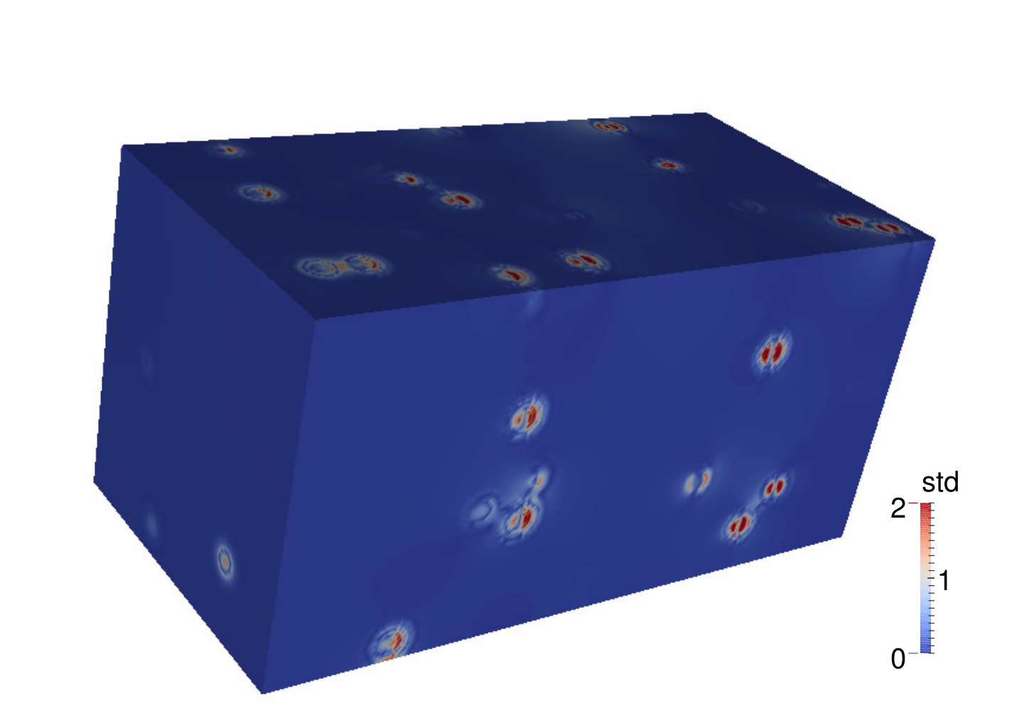
Finally, we visually compare the error in the ROM with the space-time varying confidence measure. Figure 9 displays the ROM error and the confidence measure at the final time for one realization of the bubble locations and two values of the bubble radius, and . Both measures are larger near the bubble boundaries and larger near the face containing the heat source. Visualizing these measures enables such qualitative observations and comparisons.



4.5 Comparison with a response surface
One question that arises frequently in the context of reduced-order modeling is, if one is only interested in a scalar quantity of interest from the full PDE solution, then what is the advantage of approximating the full solution with a reduced-order model? Why not just use a scalar response surface to approximate the quantity of interest as a function of the parameters? To address this question, we compare two approaches for the parameter study in Section 4.2:
- 1.
Use a response surface to interpolate the means of each of the two quantities of interest over a range of bubble radii. We use the quantities of interest at bubble radii for to decide the form of the response surface: piecewise linear, nearest neighbor, cubic spline, or piecewise cubic Hermite interpolation (PCHIP). The response surface form with the lowest testing error is constructed from the mean quantities of interest for bubble radii for —which are the same values whose simulations are used to construct the ROM. The response surface prediction is then computed for .
- 2.
Use the ROM to approximate the temperature field on the far face at the final time for each realization of the bubble location. Then compute the two quantities of interest for each approximated far face temperature distribution, and compute a Monte Carlo approximation of the mean (i.e., a simple average).
The results of this study are shown in Figure 10. For the first quantity of interest (the average temperature over the far face), the cubic spline response surface approach adequately captures the behavior as a function of the bubble radius due to the relative smoothness of the response. However, the PCHIP response surface approximation of the second quantity of interest (the proportion of far face temperature that exceeds ) is substantially less accurate than the ROM due to the sharp transition and the low resolution in the parameter space. A global polynomial or radial basis function approximation would fare worse (e.g., exhibit Gibbs oscillations near the transition) due to the global nature of the basis. We conclude that the choice of ROM versus response surface depends on the quantity of interest. Broadly speaking, if the quantity of interest is a smooth function of the parameters, then a response surface is likely sufficient. However, if the quantity of interest is a highly nonlinear or discontinuous function of the full PDE solution, then computing such a quantity from the ROM approximation will yield better results. While it was not pertinent to this example, the ROM-based approach also provides the 95% confidence bounds for the Monte Carlo estimates, since the temperature distribution for each realization of the bubble locations is approximated.
4.6 Computational considerations
We end this section with a few notes on the experience of running 8192 large-scale simulations, transferring them to a Hadoop cluster, and building the reduced-order model.
Each heat transfer simulation took approximately four hours using eight processors on Sandia’s Red Sky. Communication times were negligible, but some runs required multiple tries due to occasional network failures. Also, some runs had to be duplicated due to node failures and changes in the code paths. Each mesh with its own conductivity field took approximately twenty minutes to construct using Cubit after substantial optimizations. Unreliable network data transmissions and bursty data write patterns (e.g., one hundred jobs on Red Sky simultaneously transferring data to the Stanford cluster) forced us to write custom codes to validate the data transfer.
Working with the simulation data involved a few pre- and post-processing steps, such as interpreting 4TB of Exodus II files from Aria. The preprocessing steps took approximately 8-15 hours. We collected precise timing information, but we do not report it as these times are from a multi-tenant, unoptimized Hadoop cluster where other jobs with sizes ranging between 100GB and 2TB of data sometimes ran concurrently. Also, during our computations, we observed failures in hard disk drives and issues causing entire nodes to fail. Given that the cluster has 40 cores, these calculations consumed at most 2400 cpu-hours—compared with the 262144 cpu-hours it took to compute 8192 heat transfer simulations on Red Sky. Thus, evaluating the ROM was about 100 times faster than computing a full simulation.
We did not compare our Hadoop implementation with an MPI implementation. The dominant bottleneck in the evaluation of the ROM is the data I/O involved in processing 4TB of simulation data into a 2.3TB matrix, computing its SVD, writing it to disk, computing the interpolants, and writing those outputs back to Exodus II files. We expect that any MPI implementation would take at least 3-4 hours based on pure I/O considerations (assuming around 1GB/sec sustained data transfer speeds). It would also be substantially more complicated to implement. We used Hadoop primarily for the ease of use of its programming model.
Although MapReduce is an appealing paradigm for computing factorizations of tall matrices, the Hadoop MapReduce ecosystem has not developed simple tools for working with large databases of spatio-temporal data. For instance, writing ad hoc utilities to extract data from Exodus II files and utilities for simply stated queries like, retrieve all values of temperature with and , occupied much of the second and third authors’ time (see the mr-exodus2farface.py code in the online code for this particular script). We see many opportunities for high-impact software designed to address the mundane details of manipulating and analyzing large databases of spatio-temporal simulation data.
5 Summary & conclusions
We presented a method for building a reduced-order model of the solution of a parametererized partial differential equation. The method is based on approximating the factors of a singular value expansion of the solution using the elements of a singular value decomposition of a matrix whose columns are spatio-temporally discretized solutions at different parameter values. The SVD step compares to reduced basis methods, which project the governing equations with a subset of the left singular vectors to create small system whose solution yields the coefficients of the reduced-order model. In contrast, our method interpolates the right singular vectors in the parameter space to compute the coefficients of the ROM. By examining the gradient of the right singular vectors as the index increases, we determine a separation between factors we can accurately interpolate and those whose oscillations are too rapid to be represented on the parameter grid. This separation yields a mean prediction and a prediction covariance for each point in the spatio-temporal domain—similar to Gaussian process regression models. We use Hadoop/MapReduce to implement the ROM including the communication-avoiding, tall-and-skinny SVD, which enables the computation to scale to outputs from large-scale high-fidelity models.
We tested the model reduction method on a parameter study of large-scale heat transfer in random media. We compared the results of the ROM with a standard response surface method for approximating the scalar quantities of interest, and we found that while the cheaper response surface was appropriate for a smooth quantity of interest, the ROM was better at approximating a quantity of interest with a sharp transition in the parameter space. The 8192 heat transfer simulations used in the study generated approximately 4 TB of data. In the course of the study, we applied the MapReduce-based SVD computation to a matrices with approximately 600 GB and 2.2 TB of data. We found that existing MapReduce tools for working with such large-scale simulation data lack robustness and generality. There is an opportunity in computational science to create better tools to further simulation-based scientific exploration.
6 Acknowledgments
We thank the anonymous reviewers for helpful comments and suggestions. We also thank Margot Gerritsen at Stanford’s Institute for Computational and Mathematical Engineering for procurement of and access to the Hadoop cluster. We thank Austin Benson at Stanford for his superb code development for the TSQR and TSSVD. We thank Joe Ruthruff at Sandia for his efforts developing the infrastructure to run the Aria cases. Finally, we thank David Rogers at Sandia and acknowledge the funding of Sandia’s Computer Science Applied Research (CSAR) and the Advanced Simulation and Computing (ASC) programs. Sandia is a multiprogram laboratory operated by Sandia Corporation, a Lockheed Martin Company, for the United States Department of Energy under contract DE-AC04-94AL85000.
7 Appendix
The tables with material properties for foam and steel.
| Foam () | |
|---|---|
| (K) | (W/mK) |
| 303 | 0.0486 |
| 523 | 0.0706 |
| Steel () | |
|---|---|
| (K) | (W/mK) |
| 273 | 13.4 |
| 373 | 16.3 |
| 773 | 21.8 |
| 973 | 26.0 |
| Foam () | |
|---|---|
| (K) | (J/kgK) |
| 296 | 1269 |
| 323 | 1356 |
| 373 | 1497 |
| 423 | 1843 |
| 473 | 1900 |
| 523 | 2203 |
| Steel () | |
|---|---|
| (K) | (J/kgK) |
| 273 | 502 |
| 673 | 565 |
References
- [1] C Audouze, F De Vuyst, and PB Nair, Reduced-order modeling of parameterized pdes using time-space-parameter principal component analysis, International journal for numerical methods in engineering, 80 (2009), pp. 1025–1057.
- [2] Christophe Audouze, Florian De Vuyst, and Prasanth B Nair, Nonintrusive reduced-order modeling of parametrized time-dependent partial differential equations, Numerical Methods for Partial Differential Equations, (2013).
- [3] Ivo Babuška, Fabio Nobile, and Raúl Tempone, A stochastic collocation method for elliptic partial differential equations with random input data, SIAM Journal on Numerical Analysis, 45 (2007), pp. 1005–1034.
- [4] Peter Benner, Serkan Gugercin, and Karen Willcox, A survey of model reduction methods for parametric systems, tech. report, Max Planck Institute Magdeburg, 2013.
- [5] Austin Benson, David F. Gleich, and James Demmel, Direct tall-and-skinny QR factorizations in mapreduce architectures, arXiv, cs.DC (2012), p. 1301.1071.
- [6] Ted D Blacker, WJ Bohnhoff, and TL Edwards, Cubit mesh generation environment. volume 1: Users manual, tech. report, Sandia National Labs., Albuquerque, NM (United States), 1994.
- [7] L Susan Blackford, ScaLAPACK user’s guide, vol. 4, Society for Industrial and Applied Mathematics, 1997.
- [8] T. Bui-Thanh, K. Willcox, and M. Damodaran, Applications of proper orthogonal decomposition for inviscid transonic aerodynamics, tech. report, MIT, 2003. http://hdl.handle.net/1721.1/3694.
- [9] Tan Bui-Thanh, Karen Willcox, and Omar Ghattas, Model reduction for large-scale systems with high-dimensional parametric input space, SIAM Journal on Scientific Computing, 30 (2008), pp. 3270–3288.
- [10] Kevin Carlberg, Charbel Farhat, Julien Cortial, and David Amsallem, The GNAT method for nonlinear model reduction: effective implementation and application to computational fluid dynamics and turbulent flows, Journal of Computational Physics, (2013).
- [11] Tony F Chan, An improved algorithm for computing the singular value decomposition, ACM Transactions on Mathematical Software (TOMS), 8 (1982), pp. 72–83.
- [12] Cloudera, Hadoop version 0.20.2 in cloudera hadoop distribution version cdh3u4. http://www.cloudera.com, 2012.
- [13] Paul G Constantine and David F Gleich, Tall and skinny qr factorizations in mapreduce architectures, in Proceedings of the second international workshop on MapReduce and its applications, ACM, 2011, pp. 43–50.
- [14] Paul G Constantine and Qiqi Wang, Residual minimizing model interpolation for parameterized nonlinear dynamical systems, SIAM Journal on Scientific Computing, 34 (2012), pp. A2118–A2144.
- [15] Jeffrey Dean and Sanjay Ghemawat, MapReduce: Simplified data processing on large clusters, in Proceedings of the 6th Symposium on Operating Systems Design and Implementation (OSDI2004), 2004, pp. 137–150.
- [16] James Demmel, Laura Grigori, Mark Hoemmen, and Julien Langou, Communication-optimal parallel and sequential qr and lu factorizations, SIAM Journal on Scientific Computing, 34 (2012), pp. A206–A239.
- [17] Jennifer Goss and Kamesh Subbarao, Inlet shape optimization based on pod model reduction of the euler equations, AIAA, 5809 (2008), p. 2008.
- [18] PC Hansen, Computation of the singular value expansion, Computing, 40 (1988), pp. 185–199.
- [19] Per Christian Hansen, Discrete inverse problems: insight and algorithms, vol. 7, Society for Industrial and Applied Mathematics, 2010.
- [20] Per Christian Hansen, Misha Elena Kilmer, and Rikke Høj Kjeldsen, Exploiting residual information in the parameter choice for discrete ill-posed problems, BIT Numerical Mathematics, 46 (2006), pp. 41–59.
- [21] Bingsheng He, Wenbin Fang, Qiong Luo, Naga K. Govindaraju, and Tuyong Wang, Mars: a mapreduce framework on graphics processors, in Proceedings of the 17th international conference on Parallel architectures and compilation techniques, PACT ’08, New York, NY, USA, 2008, ACM, pp. 260–269.
- [22] Kyunghoon Lee, Taewoo Nam, Christopher Perullo, and Dimitri N Mavris, Reduced-order modeling of a high-fidelity propulsion system simulation, AIAA journal, 49 (2011), pp. 1665–1682.
- [23] John L Lumley, Gahl Berkooz, and Clarence W Rowley, Turbulence, coherent structures, dynamical systems and symmetry, Cambridge University Press, 2012.
- [24] Hung V Ly and Hien T Tran, Modeling and control of physical processes using proper orthogonal decomposition, Mathematical and computer modelling, 33 (2001), pp. 223–236.
- [25] Daisuke Mori, Yusaku Yamamoto, and Shao-Liang Zhang, Backward error analysis of the allreduce algorithm for householder qr decomposition, Japan Journal of Industrial and Applied Mathematics, 29 (2012), pp. 111–130.
- [26] P.K. Notz, S.R. Subia, M.M. Hopkins, H.K. Moffat, and D.R. Noble, Aria 1.5: User manual, Tech. Report SAND2007-2734, Sandia National Laboratories, Albuquerque, NM 87185 and Livermore, CA 94551, Apr. 2007.
- [27] Ziemowit Ostrowski, Ryszard A Białecki, and Alain J Kassab, Estimation of constant thermal conductivity by use of proper orthogonal decomposition, Computational Mechanics, 37 (2005), pp. 52–59.
- [28] Steven J. Plimpton and Karen D. Devine, Mapreduce in mpi for large-scale graph algorithms, Parallel Computing, 37 (2011), pp. 610–632.
- [29] Carl Edward Rasmussen, Gaussian processes for machine learning, (2006).
- [30] Justin Talbot, Richard M. Yoo, and Christos Kozyrakis, Phoenix++: modular mapreduce for shared-memory systems, in Proceedings of the second international workshop on MapReduce and its applications, MapReduce ’11, New York, NY, USA, 2011, ACM, pp. 9–16.
- [31] Various, Hadoop version 0.20, cloudera cdh3. http://hadoop.apache.org, http://cloudera.com, 2010.
- [32] Dongbin Xiu and Jan S Hesthaven, High-order collocation methods for differential equations with random inputs, SIAM Journal on Scientific Computing, 27 (2005), pp. 1118–1139.