Adiabatic preparation of vortex lattices
Abstract
By engineering appropriate artificial gauge potentials, a Bose-Einstein condensate (BEC) can be adiabatically loaded into a current carrying state that resembles a vortex lattice of a rotating uniform Bose gas. We give two explicit, experimentally feasible protocols by which vortex lattices can be smoothly formed from a condensate initially at rest. In the first example we show how this can be achieved by adiabatically loading a uniform BEC into an optical flux lattice, formed from coherent optical coupling of internal states of the atom. In the second example we study a tight binding model that is continuously manipulated in parameter space such that it smoothly transforms into the Harper-Hofstadter model with flux per plaquette.
pacs
67.85.-d,03.75.Lm,03.65.VfI Introduction
One of the most striking signatures of the quantum coherence of a Bose-Einstein condensate (BEC) is the formation of a lattice of quantized vortices when the condensate is forced to rotate [1, 2]. In the rotating frame of reference, the particles experience a Coriolis force which plays the same role as the Lorentz force on a charged particle in a uniform magnetic field. Hence, the vortex lattice of a rotating BEC has similar origin to the vortex lattice of a superconductor in a magnetic field. The density of vortex lines is set by the (effective) magnetic flux density, which is for atoms of mass rotating at angular frequency .
There are two common ways in which to form a vortex lattice. In one method, commonly used in superconductors, one starts from the normal (uncondensed) phase already subjected to the magnetic field. On cooling, the system undergoes a phase transition directly into the superfluid (condensed) phase with a vortex lattice of non-zero density . In another method, commonly used for liquid helium [3] and for dilute atomic gases, the system is first cooled into the condensed phase in the absence of any effective magnetic field, . The effective magnetic field is then gradually increased, for example by imposing a rotating deformation. As the field strength increases, vortices must enter from outside the condensate [4, 5, 6, 7]. For atomic BECs, this is achieved via surface wave instabilities and involves an interesting and complex dynamical evolution [8, 9, 10], including periods in which the vortex lattice is highly disordered and far from equilibrium. Nevertheless, by transfer of energy from the disordered vortex lattice into phonon modes (i.e. heating of the BEC) or by additional evaporative cooling, the system can be stabilised into ordered arrays of vortices. This has been shown in various experiments, using rotation or Raman coupling to generate the effective magnetic flux density [4, 5, 11, 6].
In this paper we describe a novel alternative route to creating a dense vortex lattice in an atomic BEC: by adiabatic manipulation of optical lattice potentials with artificial gauge fields. Recently, new ways to create strong magnetic fields for cold atoms have been put forward, and are now within reach of experiments [12, 13, 14, 15, 17, 16, 18, 19, 20, 21, 22, 23]. These methods lead to very high flux densities, about two orders of magnitude larger than previous experimental works. Thus, following the standard approach for cold gases and increasing the flux density from would require a very large number of vortices to enter the system, potentially driving the system very far from equilibrium and requiring significant cooling to maintain BEC. Our proposal shows that these very dense vortex arrays can in fact be formed adiabatically, maintaining the system at ultracold temperatures without requiring any further cooling.
We describe two generic experimental protocols by which a vortex lattice can be adiabatically created from a uniform BEC. The first setup involves loading a BEC into an optical flux lattice[14, 15, 16, 17], based on the coherent (Rabi) coupling of internal atomic states. We describe the density and current patterns in the system following loading, and show that these are as expected for the dense vortex lattice. In the second part of the paper, we turn to consider the formation of vortex lattices in the Harper-Hofstadter model[24, 25] for atoms moving on a tight-binding lattice. We present an experimental protocol by which the uniform BEC for vanishing flux per plaquette can be adiabatically transformed into the vortex-lattice ground-state of a lattice with flux per plaquette.
II Optical flux lattice
We consider bosonic atoms with two internal states, which we label by the (pseudo)-spin and . The atoms are subjected to coherent optical fields which, in the rotating wave approximation, are described by the potential with the Pauli matrices acting on the internal states. The amplitudes describe the strengths of the local optical coupling of the two internal levels () and of a state-dependent potential (). Various implementations of such couplings are possible, using electronic states, hyperfine levels or even vibrational states [26, 27]. When the optical coupling is dominant (compared to the kinetic energy defined below), the internal state of the atom is restricted to the lowest energy eigenstate of , which we denote by the dressed state . In this limit, the atom moves through space adiabatically with overall wavefunction . The Berry curvature associated with spatial variations of the dressed state causes the motion of the atom, as described by the positional wavefunction , to experience an effective magnetic field [26].
An optical flux lattice is a periodic configuration of the optical fields which cause the atom to experience a non-zero number of flux quanta, , per unit cell [14]. We focus on a simple, but representative, example of an optical flux lattice, introduced in Ref. 14
| (1) |
with , , and defining three reciprocal lattice vectors in the plane. In real space, this lattice has triangular symmetry, with lattice vectors and . Within this unit cell, the lowest energy dressed state experiences flux quanta. Thus, one expects that a BEC in this lowest energy dressed state will exhibit vortices per unit cell.
The energy bands follow from the eigenstates of the Hamiltonian including the kinetic energy, . (We focus on the motion in the plane; motion normal to this plane, along , remains free particle-like and in the Bose-condensed phases we describe the atoms will simply condense in state.) The bandstructure depends on the lattice depth where . A cut through the energy bands is shown in Fig. 1 (top) for three values of . At all lattice depths, the single particle states have two degenerate minima. This degeneracy is a consequence of the discrete symmetry operations [14]
| (2) |
involving translations by and combined with spin rotations, for which . Since , energy eigenstates can be made simultaneous eigenfunctions of and , so the magnetic unit cell can be chosen to have sides and , containing flux quantum. This leads to the magnetic Brillouin zone in Fig. 1 (bottom), with reciprocal lattice spanned by and .

The states of minimum kinetic energy, which we label , are located at and . These continuously evolve into the eigenstates of with zero kinetic energy as [28].
This continuous evolution of the bandstructure with varying allows the adiabatic preparation of a BEC in the minima of the lowest band of the optical flux lattice. We consider a protocol where the lattice lasers are ramped up slowly from , thereby loading a weakly interacting BEC into the lattice. As the Rabi coupling is mixing the spin degrees of the two-component BEC, for adiabaticity, we have to ensure that as the lattice is turned on, the BEC remains in the mean-field ground-state. Consider, first, non-interacting bosons in an ideal infinite (untrapped) system. Let us start with a BEC of spin- atoms, that is with condensate wave function
where is the number of atoms per area . Now, increasing from zero will causes the condensate wavefunction to evolve continuously into that of the state, thereby adiabatically loading the atoms into a BEC in this minimum. Similarly, a BEC in any initial superposition of spin- and spin- will evolve into a BEC in a superposition state of the degenerate minima at . For a finite system in a trap, when is nonzero the trap potential can cause scattering of particles between the two degenerate minima. Then, other considerations are required in order to ensure adiabatic loading of the BEC. One way to achieve adiabaticity is to detune the laser(s) providing the Rabi coupling from resonance by an amount . This adds a spatially uniform term to the optical coupling (1) which breaks the degeneracy of the two minima. The lowest energy band has a single non-degenerate minimum for all lattice depths, which may be adiabatic loaded without sensitivity to scattering processes. Alternatively, one can make use of the fact that inter-particle interactions can lift the degeneracy of BECs with two internal states. Specifically, we consider the effects of state-dependent interactions, for which the mean-field interaction energy is given by
| (6) |
where are the spin- densities of the condensate wave functions and / () are the intra- (inter-) species interactions. Under the assumption of weak interactions, the condensate wave function is a linear combination of the two degenerate minima, . The relative sizes of the state-dependent interactions determine the spin-state of the lowest energy BEC. For simplicity, consider the regime where
| (7) |
Then, for the lowest energy BEC involves a condensate with only , as in Eq (II). This condensate wave function minimizes the interaction energy of the free Bose gas. As above, the condensed state continuously evolves with increasing remaining the mean-field ground-state of the lattice potential.
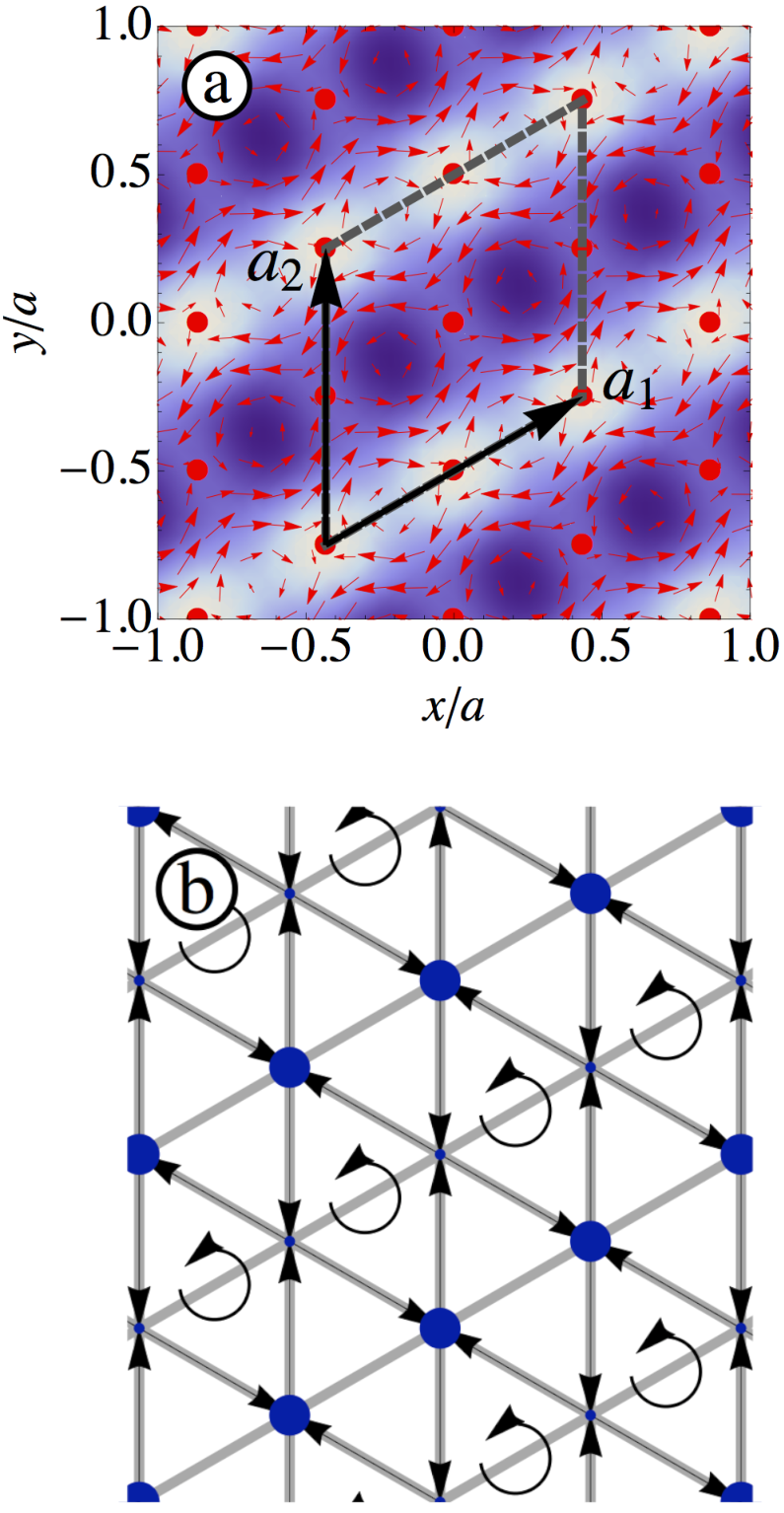
In Fig. 2 we show the condensate wavefunction formed by adiabatically loading a BEC into the -minimum, to a lattice depth of . This Figure shows both the particle density (shading) and the current density (arrows). An inspection of the pattern of densities and currents shows that these have the expected features of a vortex lattice. In the unit cell of sides the lowest energy dressed state experiences flux quanta, so we expect that there should appear 2 quantized vortices. Indeed, clear signatures of these 2 vortices appear: there are two points around which the current circulates (in an anticlockwise sense) and at the centre of which the particle density falls to a small value. There are also two stagnation points, around which the current density circulates in a clockwise sense. These are required by periodicity of the flow field (in the rest frame of the vortex lattice there is no net flow), so appear also for a rotating superfluid. They are not quantized vortices (or antivortices) since the particle density remains large at the centres of these points, so the velocity field is regular and has zero net circulation around these points.
It is clear from Fig. 2 that the vortices do not form a triangular lattice, familiar for rotating BECs. Rather, the vortices are arranged in a rectangular array. This is due to the fact that the dominant energy is the lattice potential, so the vortices arrange in order to minimize the energy of the optical coupling (1). The rectangular arrangement of the vortices leads to a particle density with a stripe-like variation in the direction perpendicular to the vector . This reflects the fact that, when condensed in the Bloch wavefunction at the minimum, the atoms have large magnetization along the -direction. The energy of the optical coupling (1) is minimized by the pinning of the density wave with density maxima along lines where .
Since the formation of the vortex is adiabatic, as the lattice depth is ramped up the density modulation and current pattern both grow smoothly and continuously, starting from uniform density and vanishing current for .

To quantify the mass flow in the flux lattice, we study the (gauge invariant) total mass current density
| (8) |
where . To demonstrate that currents smoothly increase from zero, we plot as a measure of flow the line integral of along the edges of the contour (see the inset to Fig. 3)
| (9) |
As can be seen in Fig. 3, the currents increase continuously from zero as the lattice depth is increased, thus demonstrating the adiabatic creation of a vortex lattice.
How can a vortex lattice of fixed density ( per unit cell) build up continuously? This might seem impossible. After all, recall that a quantized vortex is associated with a singularity at the vortex core (point-like in two-dimensions or line-like in three dimensions) at which the condensate density vanishes. How can one smoothly transform from a uniform BEC into a vortex lattice with zeroes in the density? The resolution lies in the fact that it is only for a one-component superfluid that the vortex core need have vanishing density. For a two- (or more-) component superfluid it is possible for the particle density to remain non-zero everywhere, in so-called “coreless vortices” [29, 30, 31]. For the optical flux lattice, in general the condensate has a two-component wavefunction, which we may write in terms of the two dressed states ( and ). For any finite lattice depth this two-component condensate has coreless vortices, so the density does not vanish at the vortex core. (In Fig. 3, is finite so, although strongly suppressed, the density remains non-zero at the vortex cores.) As the lattice depth is increased, the density suppression at the vortex core gradually develops. In the limit for which , the condensate is a one-component function which must have zeros at the vortex core.
In addition to the developing vortex core, in the limit the scalar potential experienced by the lowest energy dressed state causes the atoms to become tightly confined to lattice sites of a triangular lattice (with spacings ). In this limit, the optical flux lattice maps onto a triangular tight-binding lattice model with flux per plaquette [14]. The tight-binding limit of the condensate wavefunction in the optical flux lattice is shown in Fig. 2 (b). The vortices reside along rows of reduced density as marked by the arrows with one vortex per 4 lattice sites.
III Tight binding model
We will now describe a complementary protocol for adiabatically transforming a condensate in a tight binding lattice into a vortex lattice.
Now consider a condensate subjected to a deep optical lattice (without any applied artificial gauge potentials), in such a way that the atomic motion is well described by hopping between states localized at the lattice sites. As we will show below, by turning on appropriate photon assisted hoppings [32] between nearest neighbour lattice sites, the mean-field ground-state can be smoothly evolved into the ground-state of the Harper-Hofstadter model. We will focus on a square lattice with flux per plaquette. As a consequence of magnetic translation invariance, the single particle states for a lattice with flux per plaquette are -fold degenerate. The mean-field condensate wave function for a weakly interacting BEC is a linear superposition of the Bloch states at the minima of the dispersion relation. The (infinite) degeneracy of all different superposition states is lifted by interactions. We assume that interactions are sufficiently weak that the atoms only occupy states in the three degenerate minima. Minimizing a mean-field on-site repulsive interaction favours a condensate with uniform density, giving rise to a ground-state with rows of vortices along the diagonal of the square lattice with one vortex per three lattice sites [33, 34, 35]. The infinite degeneracy is lifted, and replaced by a residual six-fold degeneracy, arising from transformations of the vortex lattice configuration by translations and rotations by [36].
Our goal is to describe a protocol by which smooth variations of experimentally controlled parameters adiabatically transform a condensate in the lattice without gauge potential into the mean-field ground states shown in Fig. 5 (a). Care is required to ensure that the adiabatic route takes the system directly into one of the six (degenerate) ground states that are favoured by repulsive interaction. We achieve this by following a route which breaks translational symmetry in such a way that the system is guided directly into a chosen vortex lattice configuration. To this end, we consider a square lattice tight binding model with Hamiltonian
| (10) |
where are bosonic destruction (creation) operators with the integers labelling the site in the directions respectively. For flux per plaquette, the hopping matrix elements along can be chosen as
with real setting also the (uniform) hopping matrix elements along the -axis. This particular gauge is the most straightforward to implement experimentally when using photon assisted tunneling as described in Refs. [18, 20]. Additional control of the tunneling matrix elements can be achieved by combining this with a second source of photon-assisted hopping, but with spatially uniform phase pattern [37], which can be achieved by shaking the lattice along the -axis [38] or alternatively by lattice modulation. The combined effects lead to net tunneling matrix elements
| (15) |
where is the relative phase of the two drives.
For dimensionless parameter this is simply the nearest neighbour tight-binding model on a square lattice with no net flux. (The phase can be removed by a gauge transformation.) The ground state is a simple condensate without any flow. Reducing the control parameter to smoothly interpolates to the Harper-Hofstadter lattice model with flux per plaquette for which the ground state is a vortex lattice. Crucially, trajectories can be found for in the range , such that there is always a unique many-body ground state, and the system is adiabatically transferred into a stable vortex lattice phase at with high fidelity. At the final point, , the many-body state is (six-fold) degenerate, corresponding to the different translations/rotations of the vortex lattice. However energy barriers of order per particle from interactions exist between these states, preventing the formation of domains. Depending on the trajectory, the system can be prepared in different translations of the vortex lattice. For example, if we take , the hopping matrix elements take the form
with , .
To demonstrate adiabaticity, in Fig. 5 (b) we show the sum of the magnitude of the currents between lattice sites and per bond
| (20) |
as a function of . (As above, we assume that interactions are sufficiently weak that the atoms only occupy the lowest energy single particle state, which is non-degenerate for .) In the lattice with uniform flux (i.e. ), these vortex lattice states have along any bond with non-zero current (here denotes the average number of particles per lattice site). We normalized in Fig. 5 (b) by its value at , . In the more general case, while single-particle states are always non-degenerate, different choices of the relative phase will load into one of the three ground-states of the model with uniform flux shown in Fig. 5 (a) [39]. The loading process is adiabatic as long as the trajectory in -space avoids crossing the lines along with where the lowest energy single particle states changes discontinuously in -space. These ground-states, shown in Fig. 5 (a), respect the (reduced) translation symmetry of the unit cell in Fig. 4 (a) and are related by translations by one lattice site.

IV Conclusion
We have described two protocols by which artificial gauge potentials can be used to load cold bosonic atoms adiabatically into a vortex lattice. In essence our strategy is to find ways by which the single particle bandstructure interpolates between that of a free particle (or simple, non-topological, bandstructure) and that of a particle in an effective magnetic field. A BEC formed in the minimum of this band can then be adiabatically transformed into a dense vortex lattice. As we have emphasized, additional care is required when the final vortex lattice breaks a symmetry of the system (e.g. spin-rotation, or translation). Then, to prevent domain formation and ensure adiabatic loading, a route must be found which transfers the BEC directly into one of these symmetry-broken phases. We have shown how this can be done both for the optical flux lattice (by lifting the spin-degeneracy) and for the tight-binding model (by using a route which breaks the translational symmetry).
If loaded successfully into the desired ground-state vortex lattice configurations, time-of-flight expansion after rapidly turning off the optical lattice will reveal a pure condensate in a single momentum state. In the first example, this will result in peaks at momenta (with ) in the total density after expansion time . In general, time-of-flight images of cold atoms in artificial gauge potentials will be gauge dependent [6, 40, 18]. Observing a condensate in a single momentum state (rather than a linear combination of the minima) indicates that the condensate has the same translation symmetries as the implemented gauge. For example for the protocol for loading into the tight-binding lattice Eq. (III), finding a condensate in one of the three degenerate minima of the dispersion means that one of the three vortex lattice shown in Fig. 5 (a) was realized. The other three degenerate mean-field ground-states are rotated by 90∘ and have a different unit cell than the one shown in Fig. 4 (a), and therefore are superpositions of the single-particle states at the minima of the dispersion in this particular gauge. Other detection techniques would naturally rely on detecting the density wave associated with the vortex lattice, which could be detected by in-situ probes such as as light scattering or single site resolution imaging [41, 42, 43, 44].
Finally, we note that our protocols will also help to reach interesting regimes of strong correlations for bosons at high magnetic flux density. By first loading adiabatically into a dense vortex lattice at weak interaction strength and subsequently ramping to strong interactions, it may be possible to observe novel strongly correlated phases, e.g. fractional quantum Hall states of bosons in quasi-2D systems[2], which typically require low entropies.
Acknowledgements.
We are grateful to Monika Aidelsburger and Immanuel Bloch for helpful discussions and for sharing their unpublished ideas, and to Jean Dalibard for helpful comments. NRC thanks the Max Planck Institute of Quantum Optics for hospitality and the A. von Humboldt foundation for support. This work was supported by EPSRC EP/I010580/1.References
- [1] A. L. Fetter, Rev. Mod. Phys. 81, 647 (2009).
- [2] N. R. Cooper, Advances in Physics 539 (2008).
- [3] R. J. Donnelly, Quantized Vortices in Helium II (Cambridge University Press, Cambridge, 1991).
- [4] K. W. Madison, F. Chevy, W. Wohlleben, and J. Dalibard, Phys. Rev. Lett. 84, 806 (2000).
- [5] C. Raman, J. R. Abo-Shaeer, J. M. Vogels, K. Xu, and W. Ketterle, Phys. Rev. Lett. 87, 210402 (2001).
- [6] Y. J. Lin, R. L. Compton, K. Jimenez-Garcia, J. V. Porto, and I. B. Spielman, Nature (London) 462, 628 (2009).
- [7] S. Sinha and Y. Castin, Phys. Rev. Lett. 87, 190402 (2001).
- [8] F. Dalfovo and S. Stringari, Phys. Rev. A 63, 011601 (2000).
- [9] D. L. Feder, A. A. Svidzinsky, A. L. Fetter, and C. W. Clark, Phys. Rev. Lett. 86, 564 (2001).
- [10] C. Lobo, A. Sinatra, and Y. Castin, Phys. Rev. Lett. 92, 020403 (2004).
- [11] V. Schweikhard, I. Coddington, P. Engels, V. P. Mogendorff, and E. A. Cornell, Phys. Rev. Lett. 92, 040404 (2004).
- [12] D. Jaksch and P. Zoller, New J. Phys. 5, 56 (2003).
- [13] F. Gerbier and J. Dalibard, New J. Phys. 12, 033007 (2010).
- [14] N. R. Cooper, Phys. Rev. Lett. 106, 175301 (2011).
- [15] N. R. Cooper and J. Dalibard, Europhys. Lett. 95, 66004 (2011).
- [16] G. Juzeliūnas, I. B. Spielman, New J. Phys. 14 123022 (2012)
- [17] N. R. Cooper and J. Dalibard, Phys. Rev. Lett. 110, 185301 (2013).
- [18] A. R. Kolovsky, Europhys. Lett. 93, 20003 (2011).
- [19] M. Aidelsburger, M. Atala, S. Nascimbène, S. Trotzky, Y.-A. Chen, and I. Bloch, Phys. Rev. Lett. 107, 255301 (2011).
- [20] M. Aidelsburger, M. Atala, S. Nascimbène, S. Trotzky, Y.-A. Chen, and I. Bloch, arXiv:1212.2911 (2012).
- [21] J. Struck, C. Ölschläger, M. Weinberg, P. Hauke, J. Simonet, A. Eckardt, M. Lewenstein, K. Sengstock, and P. Windpassinger, Phys. Rev. Lett. 108, 225304 (2012).
- [22] K. Jiménez-García, L. J. LeBlanc, R. A. Williams, M. C. Beeler, A. R. Perry, and I. B. Spielman, Phys. Rev. Lett. 108, 225303 (2012).
- [23] P. Hauke, O. Tieleman, A. Celi, C. Ölschläger, J. Simonet, J. Struck, M. Weinberg, P. Windpassinger, K. Sengstock, M. Lewenstein, and A. Eckardt, Phys. Rev. Lett. 109, 145301 (2012).
- [24] P. G. Harper, Proc. Phys. Soc. A 68, 874 (1955).
- [25] D. R. Hofstadter, Phys. Rev. B 14, 2239 (1976).
- [26] J. Dalibard, F. Gerbier, G. Juzeliūnas, and P. Öhberg, Rev. Mod. Phys. 83, 1523 (2011).
- [27] C. V. Parker, L.-C. Ha, and C. Chin, arXiv:1305.5487 (2013).
- [28] For example, for a shallow lattice , the wavefunctions are and , where .
- [29] N. D. Mermin and T.-L. Ho, Phys. Rev. Lett. 36, 594 (1976).
- [30] T.-L. Ho, Phys. Rev. Lett. 81, 742 (1998).
- [31] T. Ohmi and K. Machida, J. Phys. Soc. Jpn. 67, 1822 (1998).
- [32] A. Eckardt, T. Jinasundera, C. Weiss, and M. Holthaus, Phys. Rev. Lett. 95, 200401 (2005).
- [33] J. P. Straley and G. M. Barnett, Phys. Rev. B 48, 3309 (1993).
- [34] S. Powell, R. Barnett, R. Sensarma, and S. Das Sarma, Phys. Rev. Lett. 104, 255303 (2010).
- [35] S. Powell, R. Barnett, R. Sensarma, and S. Das Sarma, Phys. Rev. A 83, 013612 (2011).
- [36] J. Zhang, C.-M. Jian, F. Ye, and H. Zhai, Phys. Rev. Lett. 105, 155302 (2010).
- [37] I. Bloch, private communication.
- [38] C. Sias, H. Lignier, Y. P. Singh, A. Zenesini, D. Ciampini, O. Morsch, and E. Arimondo, Phys. Rev. Lett. 100, 040404 (2008).
- [39] The other three configurations would be formed by changing the photon assisted tunneling , such that its phase is constant along lines of constant .
- [40] G. Möller and N. R. Cooper, Phys. Rev. A 82, 063625 (2010).
- [41] J. Javanainen and J. Ruostekoski, Phys. Rev. A 52, 3033 (1995).
- [42] T. A. Corcovilos, S. K. Baur, J. M. Hitchcock, E. J. Mueller, and R. G. Hulet, Phys. Rev. A 81, 013415 (2010).
- [43] W. S. Bakr, J. I. Gillen, A. Peng, S. Fölling, and M. Greiner, Nature (London)462, 74 (2009).
- [44] J. F. Sherson, C. Weitenberg, M. Endres, M. Cheneau, I. Bloch, and S. Kuhr, Nature (London)467, 68 (2010).
- [45] Petrov, D. S. and Shlyapnikov, G. V., Phys. Rev. A 64, 012706 (2001).