A temporal logic approach to modular design of synthetic biological circuits

Ezio Bartocci Affiliation: Vienna University of Technology, Austria Luca Bortolussi Affiliation: DMG, University of Trieste, Italy Affiliation: CNR/ISTI, Pisa, Italy Laura Nenzi Affiliation: IMT, Lucca, Italy

Abstract

¹¹ 1 The final pubblication is available at link.springer.com

We present a new approach for the design of a synthetic biological circuit whose behaviour is specified in terms of signal temporal logic (STL) formulae. We first show how to characterise with STL formulae the input/output behaviour of biological modules miming the classical logical gates (AND, NOT, OR). Hence, we provide the regions of the parameter space for which these specifications are satisfied. Given a STL specification of the target circuit to be designed and the networks of its constituent components, we propose a methodology to constrain the behaviour of each module, then identifying the subset of the parameter space in which those constraints are satisfied, providing also a measure of the robustness for the target circuit design. This approach, which leverages recent results on the quantitative semantics of Signal Temporal Logic, is illustrated by synthesising a biological implementation of an half-adder.

Keywords: Synthetic Biology, Parameter Synthesis, Temporal Logic.

1 Introduction

Synthetic Biology [14, 27] is an emerging discipline that aims at the rational design of artificial living systems with a predictable behaviour, either by creating new biological entities that do not exist in nature or by redesigning the existing ones. Even though important technological developments have been achieved in this field, the de-novo design of biological circuits implementing a desired behaviour results to be a very hard task, especially for large scale networks. Biological systems are complex to understand and to be engineered: the non-linear nature of interactions reflects in the emergence of systemic behavioural properties, not directly derivable from the knowledge of the individual parts. To model and control such systems we need to understand the relationships between the emergent behaviour and the topology of such complex interactions. A possible approach is to divide the whole system in “subunits” and to look at the structure of the interactions between them. This subdivision is often suggested by the way we describe (the components of) those systems. The idea is that compositionality at the specification level, to a certain extent, has to be reflected into compositionality at the behavioural level. This should depend on the properties satisfied by a single “subunit” and on the wiring between them. This way to approach the study of a system is called modularity and the “subunits” of the system are called modules. Modularity can be effectively achieved in Synthetic Biology, combining a bottom-up [31] and a top-down [30] methodology. The former consists in the assembling of a set of well-characterised modules [31] together to build sophisticated biological circuits and devices. The latter [30] aims to identify and characterise the possible “subunits” and this is also helpful to understand real biological systems, for example to discover unknown structures or behaviours or to better understand and test current knowledge.

To unveil the system dynamics, it is important to correlate the denotation of a module with some of its specific behaviours, and understand how the global properties emerge from these local ones. This can be performed better if the emergent behaviours are specified in a formal language. We consider here a logical characterisation in terms of (linear) temporal logic formulae. In particular, we focus our attention on genetic regulatory circuits, seen as networks of interacting genetic modules (each representing, for instance, a logic gate). Each module has a set of inputs and outputs (usually transcription factors), and its local behaviour is specified by temporal logic properties.

In particular, we characterise the behaviour of logic gates with the addition of constraints on the response time. Logic gates are physical devices implementing a boolean function and they are the fundamental bricks upon which all the other logic circuits, including multiplexers, arithmetic logic units, memories and microprocessors, are built. They are primarily implemented using electronic transistors acting as electronic switches. In the last decade, genetic circuits acting as logic gates have been successfully identified and synthesised [22]. This lead researchers to hope to engineer cells to turn them into miniature computers.

The main idea of this paper, sketched in Figure 1, is to translate the structural compositionality of networks of modules into compositionality of local behaviours, exploting it to enforce a set of global behaviours to the network. This is realised by identifying a subset of parameters for which the truth of local properties implies the truth of the global specification, exploiting the modular structure of the network. We thus interpret the network of modules as a composition of their local properties, connecting the emergent behaviours with the topology of interaction of those local properties. The technical core of our approach is the quantitative semantics of Signal Temporal Logic [20], which can be seen as a measure of robustness of the satisfaction of a certain formula, and which comes with simulation-based methods to compute the robustness score and to identify a region of the parameter space in which the formula holds true.

Refer to caption — Figure 1: Overview of the proposed approach.

The contributions of this paper are thus twofold: a design methodology for biological circuits based on a high level logical specification of behaviours and an algorithmic procedure exploiting compositionality to make parameter synthesis more effective, which gives as a byproduct a measure of robustness of the implementation.

The paper is structured as follows: in Section 2 we introduce the background material. In Section 3 we discuss the logical characterisation of the basic modules in terms of Signal Temporal Logic (STL). In Section 4 we sketch the algorithmic approach to parameter synthesis and in Section 5 we show an application to the design of an half-adder, a fundamental building block of microprocessors. The related works and the final discussion are in Section 6.

2 Background material

Modelling of Gene-Regulatory networks

In this paper we consider deterministic models of gene regulatory networks, given by a set of non-linear Ordinary Differential Equation (ODE) [16]. For simplicity, we consider lumped models of gene expression, in which mRNA is not explicitly represented (cf. Remark 2 for a further discussion on this point). We assume to have $n$ genes and proteins. Concentration of protein $i$ at time $t$ , $i=1,\ldots,n$ , is denoted by the variable $x_{i}[t]$ , while $\vec{x}=(x_{1},\ldots,x_{n})$ denotes the vector of concentration variables. The ODE for $x_{i}[t]$ will then be of the form

\frac{dx_{i}}{dt}=f_{i}(\vec{x})=f_{i}^{+}(\vec{x})-f_{i}^{-}(\vec{x}),

where $f_{i}^{+}$ is a function giving the net production rate of $x_{i}$ , while $f_{i}^{-}$ is its degradation rate, which is usually a linear function of the form $\mu_{i}x_{i}$ , for some $\mu_{i}>0$ . The function $f_{i}^{+}$ , instead, encodes the regulatory mechanism of gene $i$ , and is a combination of Michaelis-Menten or Hill functions [27].

Signal Temporal Logic

Temporal logic [23] provides a very elegant framework to specify in a compact and formal way an emergent behaviour in terms of time-dependent events. Among the myriads of temporal logic extensions available, Signal Temporal Logic [20] (STL) is very suitable to characterise behavioural patterns in time series of real values generated during the simulation of a dynamical system. STL extends the dense-time semantics of Metric Interval Temporal Logic [1] (MITL), with a set of parametrised numerical predicates playing the role of atomic propositions. STL provides two different semantics: a boolean semantics that returns yes/no depending if the observed trace satisfies or not the STL specification, and a quantitative semantics that in addition returns a measure of robustness of the specification. Recently, Donze et. al [11] proposed a very efficient monitoring algorithm for STL robustness, now implemented in the Breach [8] tool. The combination of robustness and sensitivity-based analysis of STL formulae have been successfully applied in several domains, ranging from analog circuits [15] to systems biology [9, 10], to study the parameter space and also to refine the uncertainty of the parameter sets. In the following we recall [12] the syntax and the quantitative semantics of STL that will be used in the rest of the paper. The boolean semantics can be inferred using the sign of the quantitative result (positive for true and negative for false).

Definition 1 (STL syntax)

The syntax of the STL is given by

\varphi:=\top\>|\>\mu\>|\>\neg\varphi\>|\>\varphi_{1}\wedge\varphi_{2}\>|\>\varphi_{1}\>\mathcal{U}_{[a,b]}\>\varphi_{2}

where $\top$ is a true formula, conjunction and negation are the standard boolean connectives, $[a,b]$ is a dense-time interval with $a<b$ and $\mathcal{U}_{[a,b]}$ is the until operator.

The atomic predicate $\mu:\mathbb{R}^{n}\rightarrow\mathbb{B}$ is defined as $\mu({\bf x}):=(y({\bf x})\geqslant 0)$ , with ${\bf x}[t]=(x_{1}[t],...,x_{n}[t])$ , $t\in\mathbb{R}_{\geqslant 0}$ , $x_{i}\in\mathbb{R}$ , and $y:\mathbb{R}^{n}\rightarrow\mathbb{R}$ a real-valued function.

The (bounded) until operator $\varphi_{1}\>\mathcal{U}_{[a,b]}\>\varphi_{2}$ requires $\varphi_{1}$ to hold from now until, in a time between $a$ and $b$ time units, $\varphi_{2}$ becomes true. The eventually operator $F_{[a,b]}$ and the always operator $G_{[a,b]}$ can be defined as usual: $F_{[a,b]}\varphi:=\top\mathcal{U}_{[a,b]}\varphi$ , $G_{[a,b]}\varphi:=\neg F_{[a,b]}\neg\varphi.$

Definition 2 (STL Quantitative Semantics)

$\displaystyle\rho(\mu,s,t)$	$\displaystyle=$	$\displaystyle\mbox{ }\phantom{a}y(s[t])\qquad\mbox{ where }\mu\equiv y(s[t])\geqslant 0$
$\displaystyle\rho(\neg\varphi,s,t)$	$\displaystyle=$	$\displaystyle\mbox{ }\phantom{a}-\rho(\varphi,s,t)$
$\displaystyle\rho(\varphi_{1}\wedge\varphi_{2},s,t)$	$\displaystyle=$	$\displaystyle\mbox{ }\phantom{a}\min(\rho(\varphi_{1},s,t),\rho(\varphi_{2},s,t))$
$\displaystyle\rho(\varphi_{1}\>\mathcal{U}_{[a,b)}\varphi_{2},s,t)$	$\displaystyle=$	$\displaystyle\mbox{ }\phantom{a}\max_{t^{\prime}\in t+[a,b]}(\min(\rho(\varphi_{2},x,t^{\prime}),\min_{t^{\prime\prime}\in[t,t^{\prime}]}(\rho(\varphi_{1},x,t^{\prime\prime}))))$

where $\rho$ is the quantitative satisfaction function, returning a real number $\rho(\varphi,s,t)$ quantifying the degree of satisfaction of the property $\varphi$ by the signal $s$ at time $t$ . Moreover, $\rho(\varphi,s):=\rho(\varphi,s,0)$ .

3 Logical characterisation of modules

The approach for the synthesis of biological circuits is based on the idea of combining simple genetic networks according to a specific design. These basic building blocks, or modules, are usually composed of a single or few genes, and express a specific transcription factor (or signal) in response to an input signal, generally the presence or absence of activators or repressors influencing the module behaviour. In most of the proposed approaches [28, 27], such modules are the biological equivalent of the logic gates of electronics, and as such they encode simple boolean functions, like AND, OR, or NOT, that can be combined together to build more complex circuits. Logic gates are usually described by their truth table. However, when moving from electronics to biology, the temporal dimension becomes much more relevant, and it cannot be neglected. Furthermore, biological modules considered in literature often produce more complex input/output (I/O) responses than a boolean I/O relationship, like pulses and oscillations [27]. For this reason, we find more convenient to describe the I/O behaviour of a module by a set of temporal logic properties.

More precisely, we define a module $\mathcal{M}$ to be a genetic network containing $n$ genes, that produce proteins whose concentration is indicated by $\vec{x}=(x_{1},\ldots,x_{n})$ . The genes of $\mathcal{M}$ are also regulated by additional $n_{I}$ external transcription factors, which are the inputs of the module. A subset of $n_{O}$ of the produced proteins constitutes the output of the module. The behaviour of such a module is characterised by a set of STL formulae of the form $\varphi_{I}\rightarrow\varphi_{O}$ , expressing an I/O relationship, which can be arbitrarily complex. Here $\varphi_{I}$ depends only on the concentration of the input signals $\mathbf{x_{I}}=(x_{I_{1}},...,x_{I_{n_{I}}})$ and $\varphi_{O}$ only on the concentration of the output signals $\mathbf{x_{O}}=(x_{O_{1}},...,x_{O_{n_{O}}})$ . Modules can be easily connected into a network, by using one output of a module as the input of another module (see Figure 2). Such networks can still have external inputs, while a subset of outputs of their modules will be identified as the output of the network. Furthermore, the network behaviour can also be characterised in terms of a temporal I/O relationship given by STL formulae of the form $\varphi_{I}\rightarrow\varphi_{O}$ . In this sense, a network is nothing but a more complex module, which can then be used as a building block itself, resulting in a hierarchical compositional approach to circuit design.

Example: Logic gates.

As an example, in this paper we consider modules corresponding to AND, OR, and NOT logic gates. For instance, a simple biological implementation of an AND gate can be obtained by a module in which a single gene, producing the output protein, is activated by two input signals, both required to start the gene expression. This requirement can be enforced directly at the level of the gene promoter [22] or by letting the complex formed by two input proteins activate the gene [19]. We stick to the first formulation. The truth table of the gate is shown in Table 1. To each input and output protein, we associate two thresholds, $\theta_{+}$ and $\theta_{-}$ . The value true in the truth table corresponds to a concentration of the corresponding protein above $\theta_{+}$ , while the value false corresponds to the concentration being below $\theta_{-}$ . In the truth table we also provide a high level specification of the temporal behaviour of the gate, in terms of the maximum response time $\delta$ and the minimum duration $\lambda$ of the output signal. The former is an upper bound on the time needed by the gate to stabilise. The latter, instead, specifies for how long the output remains up or down. This in turn implies a constraint on the duration of the input signal: if we want the output to remain up for $\lambda$ units of time, then both inputs have to remain up for at least $\lambda+\delta$ units of time. We can easily turn such a truth table into a set of STL formulae, a formula for each row. For instance, the row four of Table 2 gives:

G_{[0,\lambda+\delta]}(x_{A}\geq\theta_{A+}\wedge x_{B}\geq\theta_{B+})\rightarrow F_{[0,\delta]}G_{[0,\lambda]}(x_{C}\geq\theta_{C+}),

(1)

where $x_{A}$ and $x_{B}$ are the input signals and $x_{C}$ is the output. The mathematical model associated with this gate will be given by the non-linear ODE:

\dot{x}_{C}=H_{AND}(x_{A},x_{B},x_{C},\mathbf{k})=k_{AB}\frac{x_{A}^{n}}{K_{A}^{n}+x_{A}^{n}}\frac{x_{B}^{n}}{K_{B}^{n}+x_{B}^{n}}-k_{C}x_{C},

(2)

where $\mathbf{k}=(k_{AB},k_{C},K_{A},K_{B},n)$ is a tuple of 5 parameters: $k_{AB}$ , the maximum production rate (here we assume a zero basal expression rate), $k_{C}$ , the degradation rate, $K_{A}$ and $K_{B}$ , governing the Hill activation function, and $n$ , governing the steepness of the Hill function.

The other basic logic gates can be modelled in a similar fashion [22]: the OR gate can be obtained from the AND gate by a non-collaborative activation of gene expression (e.g., replacing in the ODE model the product of Hill functions by a single Hill function depending on the sum of the two concentrations), while the NOT gate can be modeled by a gene whose production is repressed by the input protein. For actual biological implementations, see for instance the discussion in [22, 27].

Example: XOR gate.

Figure 2 shows how to build a XOR gate using AND, OR, and NOT gates. We stress here that the circuit architecture, seen as an implementation of a boolean function, can be obtained by classical techniques (e.g. by Karnaugh maps [17]). To fully specify the extended truth table of the XOR gate, like for the AND gate (cf. Table 1), we need to specify additional information about the maximum response time and the minimal duration of the output signal for the network. These two quantities obviously depend on the corresponding ones of the constituent modules. Here we will specify a target temporal behaviour for the network and we will consequently constrain the temporal behaviour of modules.

Suppose we fix a maximum response time $\delta$ and a minimum duration $\lambda$ of the output signal for the XOR gate. Looking at Figure 2, we clearly see that the input signal to the XOR gate has to go through no more than three gates before influencing the output. Hence, if each gate has a maximum response time of $\delta/3$ , we obviously obtain a response time for the XOR bounded by $\delta$ . To enforce the constraint on the minimum duration of the output signal, we just need to make the output signals of internal gates last sufficiently long to trigger an output signal of the network of the target duration. This can be done by simply taking into account the maximum response delay of each gate. In the XOR example, we obtain that the AND gates need to have a minimal duration of $\lambda+\delta/3$ , while the NOT gates of $\lambda+2\delta/3$ . Clearly, the input signal of the network needs to stay on for $\lambda+\delta$ units of time.

Constraints for arbitrary acyclic networks of logic gates.

This simple compatibility analysis is easily generalised to arbitrary acyclic networks of logic gates, to which we restrict ourselves for the moment. Dealing with feedback loops is more complicated and is left to future investigation.

Consider a generic module/logic gate in an acyclic network, with target maximum delay $\delta$ and target output signal duration $\lambda$ . For each module $\mathcal{M}$ (with a single output) of such a network, let $\ell_{f}(\mathcal{M})$ be the length of the longest path from $\mathcal{M}$ to an output module (i.e. a module producing one output of the network) and $\ell_{b}(\mathcal{M})$ be the length of the longest path from $\mathcal{M}$ to an input module (i.e. a module with an external input). Due to the acyclic nature of the network, both such quantities are finite and can be easily computed by a visit of the graph. Then the processing of an input signal passing from $\mathcal{M}$ has to go through at most $\ell_{f}(\mathcal{M})+\ell_{b}(\mathcal{M})+1$ modules, so that a maximum delay of $\delta(\mathcal{M})=\delta/(\ell_{f}(\mathcal{M})+\ell_{b}(\mathcal{M})+1)$ guarantees the response time bound on the network. As for the minimum duration of the output for module $\mathcal{M}$ , we can obtain it by the recursive relation $\lambda(\mathcal{M})=\delta(\mathcal{M})+\max\{\lambda(\mathcal{M^{\prime}})\}$ , where $(\mathcal{M},\mathcal{M^{\prime}})$ is an edge of the network, i.e. $\mathcal{M^{\prime}}$ is a module receiving as input an output of $\mathcal{M}$ . These relationships are easily extended to modules with more than one output, defining a max response time constraint for each output.

We observe here that this compatibility analysis between delays and durations has a counterpart in the STL characterisation of module behaviours. The main idea is that we can express the consistency of the output-input links by the STL formulae like:

F_{[\nu_{1},\nu_{1}+\gamma_{1}]}G_{[0,\mu_{1}]}(x\geq\theta_{+})\rightarrow G_{[\nu_{2},\nu_{2}+\mu_{2}]}(x\geq\theta_{+}),

(3)

This formula states that if a variable is eventually expressed for $\mu_{1}$ units of time, starting between time $\nu_{1}$ and $\nu_{1}+\gamma_{1}$ , it is for sure expressed for $\mu_{2}$ units of time, starting at time $\nu_{2}$ . If we set $\mu_{1}=\lambda+\delta$ , $\mu_{2}=\lambda$ , $\gamma_{1}=\delta$ , and $\nu_{2}=\nu_{1}+\delta$ , with $\nu_{1}\geq 0$ , $\lambda,\delta>0$ arbitrary, we obtain that the formula (3) is valid. According to the previous discussion, we need to choose $\lambda=\lambda(\mathcal{M})$ and $\delta=\delta(\mathcal{M})$ .

Inputs		Output	Input $\backslash$ Output
max delay= $\delta$		min. duration= $\lambda$
pA	pB	pC	STL Formula
low	low	low	$G_{[0,\lambda+\delta]}(x_{A}\leq\theta_{A-}\wedge x_{B}\leq\theta_{B-})\rightarrow F_{[0,\delta]}G_{[0,\lambda]}(x_{C}\leq\theta_{C-})$
low	high	low	$G_{[0,\lambda+\delta]}(x_{A}\leq\theta_{A-}\wedge x_{B}\geq\theta_{B+})\rightarrow F_{[0,\delta]}G_{[0,\lambda]}(x_{C}\leq\theta_{C-})$
high	low	low	$G_{[0,\lambda+\delta]}(x_{A}\geq\theta_{A+}\wedge x_{B}\leq\theta_{B-})\rightarrow F_{[0,\delta]}G_{[0,\lambda]}(x_{C}\leq\theta_{C-})$
high	high	high	$G_{[0,\lambda+\delta]}(x_{A}\geq\theta_{A+}\wedge x_{B}\geq\theta_{B+})\rightarrow F_{[0,\delta]}G_{[0,\lambda]}(x_{C}\geq\theta_{C+})$

Table 1: Extended truth table for the AND gate

Remark 1

In principle, we can consider more complex building blocks than logic gates, for instance modules acting as switches or oscillators. To this end, we need to generalise the technique for combining modules. More specifically, effective connection of modules is enforced by requiring the validity of formula (3), which is of the form $\varphi_{O}\rightarrow\varphi_{I}$ . Such a formulation in terms of validity of STL formulae can be extended to more general output properties (or proper subformulae thereof). For instance, we can describe oscillations as signals being eventually above a high threshold for some time, and then falling below a low threshold for a subsequent period of time (this property holding globally). The subformulae describing these two behaviours can then be matched with input formulae of the kind considered in this paper.

4 Parameter synthesis

Consider a network composed by modules representing logic gates, fix a network specification in terms of an extended truth table/ STL formulae, and consider an ODE model of the network, depending on a tuple of parameters $\mathbf{k}$ . We now tackle the problem of identifying parameters $\mathbf{k}$ such that the network satisfies the specifications. According to the previous section, in order to satisfy the temporal constraints at the network level, we can simply enforce local constraints at the module level. The key intuition of our approach is that modularity can be further exploited, doing parameter synthesis for each module, with a guarantee that the so obtained parametrisation will satisfy the global specification at the network level. Furthermore, we will identify a set of compatible parameter values rather than a single point. Within the set, furthermore, we can identify an optimal parametrisation, by maximising the satisfaction level of the properties, according to STL quantitative semantics. We can also search a biological database, like BioBricks, to find genes with the synthesised kinetic constraints.

At the heart of the proposed approach resides the STL characterization of (the biological implementation of) logic gates. Essentially, we will restrict to a single gate, fixing the temporal constraints to those implied by the network requirements and by its structure, and find a subset of the parameter space in which the STL formulae characterising the gate behaviour hold true. This can be done algorithmically, using the simulation approach to parameter synthesis of [9], based on sensitivity analysis and STL quantitative semantics and implemented in Breach [8]. For the simple class of logic gates considered here, we can also do this analytically. Modularity is the key to the efficiency of our approach: as we treat independently each gate, we just need to explore a low dimensional parameter space, which makes the (computational) procedure feasible.

Modularity of parameter synthesis for logic gates.

The main difficulty we have to solve is related to the fact that modules are connected in the network, hence they are not independent. Indeed, the expression of a gene is driven by the dynamical behaviour of its input transcription factors. The idea to get around this problem is to do a worst case analysis, showing that a specific parameter combination satisfies the properties for the “worst possible input signal”, and that this implies the satisfaction for all possible input signals compatible with the input constraints. This will result in a conservative, but computationally efficient, estimate. We can define the notion of “worst case input signal” in terms of the STL characterisation of module behaviour. Given an input signal $\mathbf{x_{I}}[t]$ of a module $\mathcal{M}$ , $t\in[0,T]$ , we denote with $\mathbf{x}_{\mathbf{x_{I}},\mathbf{k}}[t]$ the trajectory of the module, with input $\mathbf{x_{I}}[t]$ and parameters $\mathbf{k}$ .

Definition 3

An input signal $\mathbf{\hat{x}_{I}}[t]$ , $t\in[0,T]$ is a worst-case input signal for the STL specification $\varphi_{Input}\rightarrow\varphi_{Output}$ of the behaviour of a module $\mathcal{M}$ if and only if, for each parameter configuration $\mathbf{k}$ such that $\rho(\varphi_{Input},\mathbf{\hat{x}_{I}})\geq 0$ (and $\varphi_{Input}$ true) and $\rho(\varphi_{Output},\mathbf{x}_{\mathbf{\hat{x}_{I}},\mathbf{k}})>0$ , the following property holds:

•

for each other input signal $\mathbf{x_{I}}$ satisfying $\rho(\varphi_{Input},\mathbf{x_{I}})\geq 0$ (and $\varphi_{Input}$ true), it holds that $\rho(\varphi_{Output},\mathbf{x}_{\mathbf{x_{I}},\mathbf{k}})\geq\rho(\varphi_{Output},\mathbf{x}_{\mathbf{\hat{x}_{I}},\mathbf{k}})$ .

The characterisation of such a “worst possible input signal” depends on the structure of the target STL formula and on the system of ODE describing a particular module. We provide now such a characterisation for the basic logic gate models considered in this paper and for the STL formulae associated with their extended truth tables.
Consider the property $G_{[0,\lambda+\delta]}(x_{A}\geq\theta_{A^{+}}\wedge x_{B}\geq\theta_{B^{+}})\rightarrow F_{[0,\delta]}G_{[0,\lambda]}(x_{C}\geq\theta_{C^{+}})$ , which describes a row of the extended truth table of an AND gate. This property is of the desired form $\varphi_{Input}\rightarrow\varphi_{Output}$ . Now, $\varphi_{Input}$ identifies a subset of trajectories of the space of functions from $[0,\lambda+\delta]$ to $\mathbb{R}^{2}$ , i.e. those that satisfy the inequality $x_{A}\geq\theta_{A^{+}}\wedge x_{B}\geq\theta_{B^{+}}$ for all $t\in[0,\lambda+\delta]$ . Among those functions, we consider $\hat{x}_{A}[t]\equiv\theta_{A^{+}}$ and $\hat{x}_{B}[t]\equiv\theta_{B^{+}}$ , which satisfy $\varphi_{Input}$ but have quantitative satisfaction score equal to zero. Furthermore, for any other trajectory $x_{A}[t],x_{B}[t]$ that satisfies $\varphi_{Input}$ , we have $x_{A}[t]\geq\hat{x}_{A}[t]$ for each $t\in[0,\lambda+\delta]$ , and similarly for $x_{B}$ . By monotonicity of Hill functions, this implies that the vector field of the AND gate satisfies $f_{AND}(x_{A}[t],x_{B}[t],x_{C},\mathbf{k})\geq f_{AND}(\hat{x}_{A}[t],\hat{x}_{B}[t],x_{C},\mathbf{k})$ for any $x_{C}\geq 0$ . It then follows, by integrating the vector field, that $x_{C}[t]\geq\hat{x}_{C}[t]$ for $t\in[0,\lambda+\delta]$ . Looking at the satisfaction function of $\varphi_{Output}$ , defined by

\rho(\varphi_{Output},x_{C})=\max_{\hat{t}\in[0,\lambda]}(\min_{t\in[\hat{t},\hat{t}+\delta]}(x_{C}[t]-\theta_{C^{+}})),

it is easy to see that $x_{C}[t]\geq\hat{x}_{C}[t]$ for $t\in[0,\lambda+\delta]$ implies $\rho(\varphi_{Output},x_{C})\geq\rho(\varphi_{Output},\hat{x}_{C})$ . Hence, any configuration of parameters such that $\rho(\varphi_{Output},\hat{x}_{C})>0$ will imply the truth of $\varphi_{Output}$ for any input signal satisfying $\varphi_{Input}$ , and therefore the truth of $\varphi_{Input}\rightarrow\varphi_{Output}$ . It follows that $\hat{x}_{A},\hat{x}_{B}$ is a worst-case input signal.

For the AND gate, a similar approach allows us to deal with the other three STL properties associated with the other rows of the truth table. In these cases, we need to find an upper bound for $x_{C}[t]$ , as we need to satisfy the output property $F_{[0,\delta]}G_{[0,\lambda]}(x_{C}\leq\theta_{C^{-}})$ . To achieve this, we just need to set $x_{J}[t]$ to $\theta_{J^{-}}$ , if the input $J$ is false, and to $\gamma_{J}$ if the input $J$ is true, where $\gamma_{J}$ is the maximum concentration level for the input $x_{J}$ , obtained by dividing maximum production rate by the degradation rate (here $J=A,B$ ). In fact, in this way we maximise the production rate. All this analysis is easily extended to OR and NOT gates, and is captured in the following proposition.

Proposition 1

Let $x_{O}$ be the output of a AND or OR logic gate and let $x_{J}$ be a generic input. Fix the attention on a row of the extended truth table.

•

If $x_{O}$ is high, and $x_{J}$ high, then $\hat{x}_{J}\equiv\theta_{J^{+}}$ .
•

If $x_{O}$ is high, and $x_{J}$ low, then $\hat{x}_{J}\equiv 0$ .
•

If $x_{O}$ is low, and $x_{J}$ high, then $\hat{x}_{J}\equiv\gamma_{J}$ .
•

If $x_{O}$ is low, and $x_{J}$ low, then $\hat{x}_{J}\equiv\theta_{J^{-}}$ .

Similarly, let $x_{O}$ be the output of a NOT logic gate²² 2 The difference between AND/ OR and NOT gates is in the fact that the input is an activator in the first two cases and a repressor in the last one. and let $x_{J}$ be its input. Then

•

If $x_{O}$ is high, then $x_{J}$ is low and $\hat{x}_{J}\equiv\theta_{J^{-}}$ .
•

If $x_{O}$ is low, then $x_{J}$ is high and $\hat{x}_{J}\equiv\theta_{J^{+}}$ .

We stress that this proposition not only allows us to do parameter synthesis modularly, but also to find a lower bound on the robustness score of each parameterization.

Remark 2

The worst case analysis presented in this section relies on the monotonicity of the robustness score with respect to the input signal. This follows from the monotone dependence of the output on the input (in fact, $\frac{\partial f}{\partial x_{J}}>0$ ), and of the robustness score on the output. The construction of the worst case input is easily generalised to more complex scenarios satisfying a generalised monotonic property of the robustness score, following [26]. As an example, consider a model of the gene expression in which the gene produces the mRNA, and mRNA is in turn translated into the protein. In this case, for an AND gate, we have an ODE for mRNA similar to the one above, namely $\frac{dm_{C}}{dt}=f_{AND}(x_{A},x_{B},m_{C},\mathbf{k})$ , while the ODE for the protein becomes $\frac{dx_{C}}{dt}=f_{C}(m_{C},x_{C},\vec{k})=k_{t}m_{C}-k_{d}x_{C}$ , with $k_{t}$ the translation constant and $k_{d}$ the protein degradation constant. The monotonic dependence of the robustness score (when both inputs are on) from inputs essentially follows because a larger input concentration will produce more mRNA, which in turn will result in a higher expression of the protein, giving a larger robustness degree (input/ output properties are the same). If such a monotonic dependence fails, determining the worst case input can be more challenging. We will tackle this issue in our future work.

Sketch of the algorithm.

Assuming the temporal constraints on the extended truth tables of modules have been derived from those of the network, the algorithm for parameter synthesis then work as follows: for any module/gate of the network, and any row in the extended truth table, fix the values of input signals to the worst case ones, and then do STL parameter synthesis to identify a subset of the parameter space in which the STL formula associated with the row is true. Take the intersection of these sets for each row in the truth table of each module³³ 3 We use the convention that parameters not influencing a gate are set to their whole domain by the STL procedure.

The STL parameter synthesis can be performed applying the sensitivity-based algorithm [9] implemented in the Matlab toolbox Breach [8]. This is a general approach, applicable to any module for which a worst-case input signal has been identified. However, for logic gates AND, OR, and NOT, we can further exploit their simplicity and characterise analytically a subset of parameters for which the STL specification is satisfied. This is due to the fact that, once the input signals are fixed, the non-linear model of the gate reduces to a linear set of ODEs, for which we can compute the solution in closed form. The details of the computation are reported in the Appendix.

5 Example: Half-Adder

The half-adder is a digital component that perfoms the sum of two bits A and B and provides two outputs, the sum (S) and the carry (C) signal representing an overflow into the next digit of a multi-digit addition. The value of the sum is 2C + S. Figure 2 a) shows the simplest half-adder design and it incorporates a XOR gate for S and an AND gate for C. Figure 2 b) shows an alternative design using two NOT gates, two AND gates and one OR gate instead of a XOR gate. This is the design of the half-adder we intend to use, thus exploiting the characterisation of worst-case inputs for AND, OR, and NOT gates given in Proposition 1. Figure 2 c) shows the output of each component gate of the half-adder, for each pair of inputs.

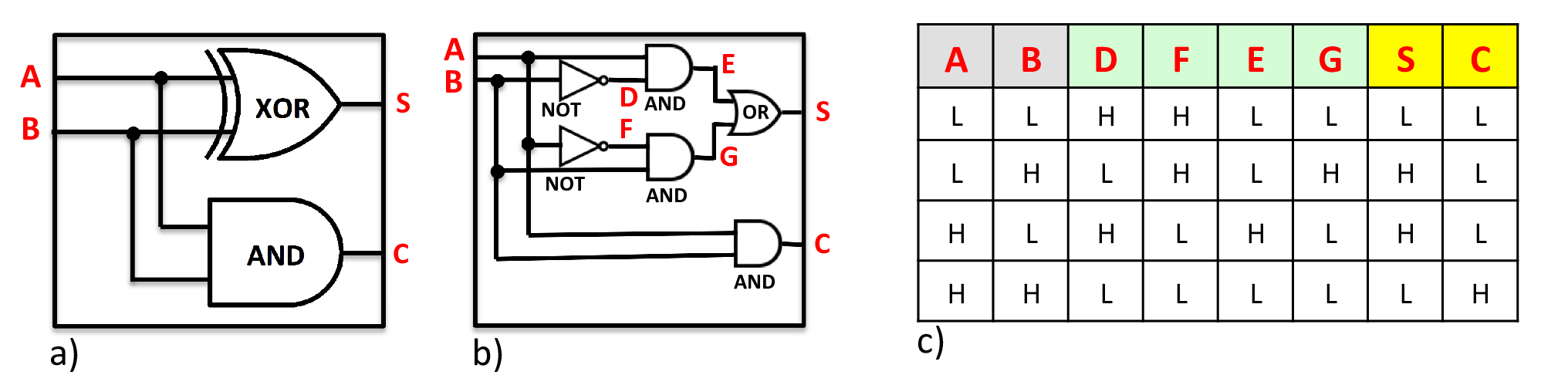
We applied the algorithm discussed in the previous section to such a network layout, fixing the maximum total delay of the half-adder to 12 time units. Applying the method to enforce time constraints to each module, we obtain that all the gates that are part of the XOR gate must have a maximum time delay of 4 time units, while the AND gate whose output is C can have a maximum response time bounded by 12 time units. Before doing parameter synthesis, we also rescaled the concentration of each protein to the interval [0,1]. In this way, activation and deactivation thresholds are relative to the maximum steady state expression level of each protein. For this example, we then arbitrarily fixed all the activation thresholds to $\theta_{+}=0.75$ and the deactivation thresholds to $\theta_{-}=0.25$ , and then synthesised set of parameters consistent with the STL network specification and with such thresholds. We obtained the following bounds for parameters, with indices in the $n$ and $\alpha$ parameters referring to the output variable and indices in the $K$ parameters referring to the input and output protein, as from Figure 2 b). AND gate: $n_{C},n_{E},n_{G}\geq 3.2129$ , $0.3406\leq K_{AC},K_{BC},K_{AE},K_{DE},K_{BG},K_{FG}\leq 0.4228$ , $\alpha_{C}\geq 0.3074$ , $\alpha_{E},\alpha_{G}\geq 0.9222$ . OR gate: $n_{S}\geq 3.1681$ , $0.4050\leq K_{ES},K_{GS}\leq 0.5090$ , $\alpha_{S}\geq 0.9222$ . NOT gates: $n_{D},n_{F}\geq 2.5372$ , $0.4192\leq K_{AF},K_{BD}\leq 0.4966$ , $\alpha_{D},\alpha_{F}\geq 0.9222$ . Constraints are similar for all gates of a given class (e.g. all AND gates) as a consequence of the rescaling of variables in [0,1]. Obviously, in a further step matching actual biological components to the circuit design, this rescaling has to be properly accounted for (for instance, by rescaling also the parameters of the biological components). Picking a value for each parameter consistent with the previous constraints, we can observe in Figure 3 that the dynamics of the network indeed satisfies the specifications of a half-adder.

We remark that, even if in this example we fixed the activation and deactivation thresholds and did parameter synthesis for the other parameters of the model, in the formal derivation we considered such threshold as parameters themselves.

6 Discussion

In this paper we focused on the design techniques for synthetic biological systems. We developed an approach based on two ideas: the specification of system properties in terms of signal temporal logic, and the exploitation of modularity to obtain an efficient procedure to identify a set of parameters for which the network satisfies its STL specification. In particular, we concentrated on the parameter synthesis problem for networks of logic gates, implemented as simple genetic networks. For acyclic networks, we are able to identify efficiently a set of parameters satisfying STL formulae encoding not only the desired boolean behaviour of the network, but also constraints on its response time.

Modularity allows us to synthesise parameters efficiently, processing each gate component independently. This is possible by isolating each module from the network assuming the worst possible input, which we formally characterised for the basic logic gates considered. We then showed the approach at work with a network implementing an half-adder.

The approach of this paper can be complemented by looking at databases of biological components, like BioBricks [18], for actual combinations of gene and promoters that satisfy the constraints on parameters. A delicate point for this plan is that we are implicitly requiring each module to produce different, non-interfering, output proteins, a not necessarily biologically realistic hypothesis. We will look at possible ways of relaxing this constraint, as in [32]. Other directions for future work include the generalisation of Proposition 1 to deal with more complex modules, for instance feed-forward networks implementing pulse generation or a low-pass filter. Moreover, we will consider the problem of dealing with more complex network topologies, having feedback loops. We expect to make some progress in this direction by suitably rephrasing parameter synthesis as the computation of a fixed point. Finally, we will also take into account the effects of stochasticity, for instance by exploiting moment closure techniques [29].

Related Work.

De novo design of a synthetic biological circuit [7] implementing a desired behaviour is a very computational intensive task. The majority of the existing approaches relies on brute-force techniques running sophisticated optimization (i.e. evolutionary algorithms [13], simulating annealing [6]) algorithms to tune the kinetic parameters [28, 5, 24] values in order to match the desired beahaviour.

These methodologies, lacking of compositionality, do not scale well and they are very computationally expensive for large networks. A more rational approach for automatic design was proposed by Marchisio and Stelling in [21, 3] where they show a workflow design taking as input a truth table and generating as output several possible circuit schemes, ranking them in the order of complexity. The choice of a truth table as a input specification for the target circuit design may be not enough when we need to guarantee that the result is produced after a proper delay. Additionally, the design needs to take in consideration the signal compatibility among the “wired” devices (a problem treated in [32]): the output signal of one device must match (in terms of low/high thresholds) with the input signal the other design. The novelty of our contribution is using signal temporal logic as specification language both for the target circuit and for the available components, adding also time constraints in the design process. Furthermore, the device compatibility is rephrased in terms of a STL formula, of the form $\varphi_{O}\rightarrow\varphi_{I}$ , and the correct matching is elegantly obtained by requiring this formula to be valid.

Another related approach, is the one proposed by Batt et al. in [2], where the authors approximate the behaviour of genetic regulatory networks with piecewise multi-affine systems. In this class of models, the state-space is partitioned in hyper-rectangles exhibiting useful convexity properties [4] that allows to compute an over-approximation of the reachable sets. The authors exploit this characteristic to guide the parameter space partitioning in search of the intervals for which the gene networks is enforced to satisfy a particular behaviour expressed in a linear temporal logic formula. However, their approach is not modular, and only the rates of production and degradation of the proteins can be chosen as possible parameters. Furthermore, by using an over-approximation, the property usually expresses invariants and the parameter ranges found are very coarse, without discriminating trajectories with different time-constraints.

Finally, among the vast literature on combinatorial circuit design, we mention [25], where authors study the timing behaviour of a acyclic circuits by means of timed automata. Our approach is simpler and motivated by the inherent precision of delays in ODE models. However, the techniques of [25] could be helpful to relax the timing constraints we impose and to deal with intrinsic variability of biochemical systems.

References

[1] R. Alur, T. Feder, and T.A. Henzinger. The benefits of relaxing punctuality. J. ACM, 1996.
[2] G. Batt, B. Yordanov, R. Weiss, and C. Belta. Robustness analysis and tuning of synthetic gene networks. Bioinformatics, 23(18):2415–2422, Sep 2007.
[3] J. Beal, R. Weiss, D. Densmore, A. Adler, E. Appleton, J. Babb, S. Bhatia, N. Davidsohn, T. Haddock, J. Loyall, R. Schantz, V. Vasilev, and F. Yaman. An End-to-End Workflow for Engineering of Biological Networks from High-Level Specifications. ACS Synth Biol, 1(8):317–331, Aug 2012.
[4] C. Belta and L.C.G.J.M. Habets. Controlling a class of nonlinear systems on rectangles. IEEE Trans. of Automatic Control, 51(11):1749–1759, 2006.
[5] B. S. Chen, C. Y. Hsu, and J. J. Liou. Robust design of biological circuits: evolutionary systems biology approach. J. Biomed. Biotechnol., 2011:304236, 2011.
[6] M. S. Dasika and C. D. Maranas. OptCircuit: an optimization based method for computational design of genetic circuits. BMC Syst Biol, 2:24, 2008.
[7] D. Densmore and J.C. Anderson. Combinational logic design in synthetic biology. In Circuits and Systems, 2009. ISCAS 2009. IEEE International Symposium on, pages 301–304, 2009.
[8] A. Donzé. Breach, a toolbox for verification and parameter synthesis of hybrid systems. In Proc. of CAV, volume 6174 of Lecture Notes in Computer Science, pages 167–170. Springer Berlin / Heidelberg, 2010.
[9] A. Donzé, G. Clermont, and C.J. Langmead. Parameter synthesis in nonlinear dynamical systems: Application to systems biology. Journal of Computational Biology, 17(3):325–336, 2010.
[10] A. Donzé, E. Fanchon, L. M. Gattepaille, O. Maler, and P. Tracqui. Robustness analysis and behavior discrimination in enzymatic reaction networks. PLoS One, 6(9):e24246, 2011.
[11] A. Donzé, T. Ferrer, and O. Maler. Efficient robust monitoring for stl. In Computer Aided Verification, volume To Appear of Lecture Notes in Computer Science. Springer Berlin / Heidelberg, 2013.
[12] A. Donzé and O. Maler. Robust satisfaction of temporal logic over real-valued signals. In Proc. of the FORMATS, pages 92–106, 2010.
[13] P. Francois and V. Hakim. Design of genetic networks with specified functions by evolution in silico. PNAS, 101(2):580–585, 2004.
[14] P. Fu and Panke S. Systems Biology and Synthetic Biology. John Wiley & Sons, 2009.
[15] K. D. Jones, Konrad V, and D. Nickovic. Analog property checkers: a ddr2 case study. Formal Methods in System Design, 36(2):114–130, 2010.
[16] H. De Jong. Modeling and simulation of genetic regulatory systems: A literature review. Journal of Computational Biology, 9:67–103, 2002.
[17] M. Karnaugh. The map method for synthesis of combinational logic circuits. Trans American Institute of Electrical Engineers, 72(2), 1953.
[18] Thomas Knight. Idempotent vector design for standard assembly of biobricks. Technical Report MIT Synthetic Biology Working Group, MIT, 2003.
[19] M. Madec, C. Lallement, Y. Gendrault, and J. Haiech. Design methodology for synthetic biosystems. In Proc. of MIXDES, pages 621–626, 2010.
[20] O. Maler and D. Nickovic. Monitoring temporal properties of continuous signals. In Proc. of FORMATS, pages 152–166, 2004.
[21] M. A. Marchisio and J. Stelling. Automatic design of digital synthetic gene circuits. PLoS Comput. Biol., 7(2):e1001083, Feb 2011.
[22] Chris J. Myers. Engineering Genetic Circuits. Chapman & Hall/CRC, 2009.
[23] Amir Pnueli. The temporal logic of programs. Foundations of Computer Science, IEEE Annual Symposium on, 0:46–57, 1977.
[24] G. Rodrigo and A. Jaramillo. AutoBioCAD: Full Biodesign Automation of Genetic Circuits. ACS Synth Biol, Nov 2012.
[25] R. B. Salah, Ma. Bozga, and O. Maler. On timing analysis of combinational circuits. In Proceedings of FORMATS, 2004.
[26] H. L. Smith. Systems of odes which generate an order preserving flow. a survey of results. SIAM Review, 30(1):87–113, 1988.
[27] Z. Szallasi, J. Stelling, and Periwal V. System Modelling in Cellular Biology: from concepts to nuts and bolts. The Mit Press, 2006.
[28] M. Terzer, M. Jovanovic, A. Choutko, O. Nikolayeva, A. Korn, D. Brockhoff, F. Zurcher, M. Friedmann, R. Schutz, E. Zitzler, J. Stelling, and S. Panke. Design of a biological half adder. Synthetic Biology, IET, 1(1.2):53–58, 2007.
[29] N. G. Van Kampen. Stochastic Processes in Physics and Chemistry. Elsevier, 1992.
[30] G. von Dassow, E. Meir, E. M. Munro, and G. M. Odell. The segment polarity network is a robust developmental module. Nature, 2000.
[31] Brynn H. Voy, Jon A. Scharff, Andy D. Perkins, Arnold M. Saxton, Bhavesh Borate, Elissa J. Chesler, Lisa K. Branstetter, and Michael A. Langston. Extracting gene networks for low-dose radiation using graph theoretical algorithms. PLoS Comput Biol, 2006.
[32] F. Yaman, S. Bhatia, A. Adler, D. Densmore, and J. Beal. Automated selection of synthetic biology parts for genetic regulatory networks. ACS Synth Biol, 1(8):332–344, Aug 2012.

Appendix 0.A Author’s contributions

L. Nenzi (PhD student at IMT, Lucca) developed the mathematical and the computational part. All authors contributed to brainstorning and to the writing.

Appendix 0.B Half-Adder, system of ODEs

The full ODE system for the Half-Adder model is:

\begin{cases}\frac{dx_{D}}{dt}=\frac{\beta_{D}}{1+(\frac{x_{B}}{K_{BD}})^{n}}-\alpha_{D}\cdot x_{D},\\ \frac{dx_{E}}{dt}=\beta_{E}\cdot\frac{x_{A}^{n}}{K_{AE}^{n}+x_{A}^{n}}\cdot\frac{x_{D}^{n}}{K_{DE}^{n}+x_{D}^{n}}-\alpha_{E}\cdot x_{E},\\ \frac{dx_{F}}{dt}=\frac{\beta_{F}}{1+(\frac{x_{A}}{K_{AF}})^{n}}-\alpha_{F}\cdot x_{F},\\ \frac{dx_{G}}{dt}=\beta_{G}\cdot\frac{x_{F}^{n}}{K_{FG}^{n}+x_{F}^{n}}\frac{x_{B}^{n}}{K_{BG}^{n}+x_{B}^{n}}-\alpha_{G}\cdot x_{G},\\ \frac{dx_{S}}{dt}=\beta_{S}\cdot\frac{(\frac{x_{E}}{K_{ES}})^{n}+(\frac{x_{G}}{K_{GS}})^{n}}{1+(\frac{x_{E}}{K_{ES}})^{n}+(\frac{x_{G}}{K_{GS}})^{n}}-\alpha_{S}\cdot x_{S},\\ \frac{dx_{C}}{dt}=\beta_{C}\cdot\frac{{x_{A}}^{n}}{K_{AC}^{n}+{x_{A}}^{n}}\cdot\frac{{x_{B}}^{n}}{K_{BC}^{n}+{x_{B}}^{n}}-\alpha_{C}\cdot x_{C},\\ x_{D}(0)=x_{D_{0}},\\ x_{E}(0)=x_{E_{0}},\\ x_{F}(0)=x_{F_{0}},\\ x_{G}(0)=x_{G_{0}},\\ x_{S}(0)=x_{S_{0}},\\ x_{C}(0)=x_{C_{0}};\end{cases}

where $A$ and $B$ are the inputs of the whole system, $D$ and $F$ are outputs of NOT gates, $E$ , $G$ and $C$ are outputs of AND gates and $S$ is the output of an OR gate.

Appendix 0.C Analytic characterisation of parameter synthesis for logic gates

If we fix the value of inputs signals, each gate (AND, NOT, OR) can be described by a linear ODE systems of the form

\begin{cases}\frac{dx}{dt}=\beta\cdot K-\alpha\cdot x,\\ x(0)=x_{0};\end{cases}

where x is the concentration of the output, $\beta>0$ is the production rate, $\alpha>0$ the degradation rate and $1\geqslant K\geqslant 0$ is the Hill term. We can rescale the systems in $[0,1]$ observing that, for each $t$ , $x(t)\leqslant\frac{\beta}{\alpha}$ , the steady state value for $K=1$ , provided $x_{0}\leqslant\frac{\beta}{\alpha}$ . Calling $\gamma=\frac{\beta}{\alpha}$ , and $\tilde{x}=x/\gamma$ , we have:

\begin{cases}\frac{d\tilde{x}}{dt}=\frac{d(\frac{x}{\gamma})}{dt}=\frac{\beta}{\gamma}\cdot K-\alpha\cdot\frac{x}{\gamma}=\alpha\cdot K-\alpha\cdot\tilde{x},\\ \tilde{x}(0)=\tilde{x}_{0};\end{cases}

The analytic solution of this equation, omitting the tilde for simplicity, is:

x(t)=K+(x_{0}-K)\cdot e^{-\alpha\cdot t}

(4)

The constraints on the dynamics expressed by STL formulas, in the simple case of constant inputs, can be translated into a systems of inequalities. As an example, consider the AND gate and the STL formula obtained from the first row of the truth table, as discussed in Section 3. The analytic solution of the AND gate equation, with initial output concentration $x_{C}(0)=0$ , (which is a lower bound on any solution with larger initial conditions, hence represents the worst case for the considered scenario) is:

x_{C}(t)=\frac{{x_{A}}^{n}}{K_{AC}^{n}+{x_{A}}^{n}}\cdot\frac{{x_{B}}^{n}}{K_{BC}^{n}+{x_{B}}^{n}}(1-e^{-\alpha\cdot t})

(5)

The STL formula for the fourth row is:

G_{[0,\lambda+\delta]}(x_{A}\geq\theta_{A^{+}}\wedge x_{B}\geq\theta_{B^{+}})\rightarrow F_{[0,\delta]}G_{[0,\lambda]}(x_{C}\geq\theta_{C^{+}}),

(6)

If we fix $x_{A}=\theta_{A^{+}},x_{B}=\theta_{B^{+}},x_{C}(0)=0$ , the formula is satisfied if and only if

F_{[0,\delta]}G_{[0,\lambda]}(x_{C}\geq\theta_{C^{+}}).

Now, the solution (5) is a monotonic increasing function converging to the steady state value $x_{C}(\infty)=K$ . It follows that if $K\geqslant\theta_{C^{+}}$ and $x(\delta)\geqslant\theta_{C^{+}}$ , the STL formula is satisfied (the second condition guarantees that the threshold is crossed no later than $\delta$ time units). In a similar way it is possible to derive a system of inequalities for all the other STL constraints considered.

Bounding the degradation constant.

We first discuss how to bound the degradation constant. In particular, we will provide a generic bound, holding for all basic logic gates considered. Fix the thresholds $\theta_{+}$ (high concentration) and $\theta_{-}$ (low concentration) for the output and the maximum time delay $\delta$ . We need to consider two cases:

•

Case $x_{0}=0$ and $x(\delta)\geqslant\theta_{{+}}$ . Here we want to upper bound by $\delta$ the time at which $x$ crosses the high concentration threshold $\theta_{+}$ . Now, for the solution $x(t)$ to eventually become bigger than the threshold $\theta_{+}$ , we need $K>\theta_{+}$ . We can enforce a stricter constraint by setting $K\geqslant\theta_{+}(1+p)$ for $p>0$ , which guarantees that the threshold is crossed in finite time. From equation 4 we get

$K(1-e^{-\alpha\delta})\geqslant\theta_{+}\qquad\mbox{ for }1\geqslant K\geqslant\theta_{+}(1+p),$

thus

$\alpha\geqslant\frac{1}{\delta}\log\left(\frac{K}{K-\theta_{+}}\right)\qquad\mbox{ for }1\geqslant K\geqslant\theta_{+}(1+p),$

This inequality holds independently of $K$ if and only if:

$\alpha\geqslant\frac{1}{\delta}\log\left(\frac{1}{p\theta_{+}}\right)$
•

Case $x_{0}=1$ and $x(\delta)\leqslant\theta_{{-}}$ . In this case, we want to upper bound by $\delta$ the time it takes for the solution to fall below the threshold $\theta_{-}<\theta_{+}$ . In this case, we require $K\leq(1-p)\theta_{-}$ , $p>0$ , so that this time is bounded. From equation (4), we obtain:

$K+(1-K)\cdot e^{-\alpha\cdot\delta}\leqslant\theta_{-}\qquad\mbox{ for }0<K\leqslant(1-p)\theta_{-},$

resulting in

$\alpha\geqslant\frac{1}{\delta}\log\left(\frac{1-K}{\theta_{-}-K}\right)\qquad\mbox{ for }0<K\leqslant(1-p)\theta_{-},$

holding independently of $K$ if and only if:

$\alpha\geqslant\frac{1}{\delta}\log\left(\frac{1}{p\theta_{-}}\right)$

As $\theta_{-}<\theta_{+}$ , intersecting the two conditions on $\alpha$ we obtain

\alpha\geqslant\frac{1}{\delta}\log\left(\frac{1}{p\theta_{-}}\right)

(7)

AND gate.

We consider now the constraints specific to an AND gate. The ODE systems of the AND gate is:

\begin{cases}\frac{dx_{C}}{dt}=\alpha_{C}\cdot\frac{{x_{A}}^{n}}{K_{AC}^{n}+{x_{A}}^{n}}\cdot\frac{{x_{B}}^{n}}{K_{BC}^{n}+{x_{B}}^{n}}-\alpha_{C}\cdot x_{C},\\ x_{C}(0)=x_{C_{0}};\end{cases}

where $x_{A}$ and $x_{B}$ are the concentrations of the inputs $A$ and $B$ , $K_{AC}$ and $K_{BC}$ are the concentration thresholds of $A$ and $B$ to activate the production of $C$ , $n$ is the Hill coefficient.

According to the discussion of the paper, we will fix the value of $x_{A}$ and $x_{B}$ to a constant, either their activation thresholds $\theta_{A^{+}}$ and $\theta_{B^{+}}$ , or their deactivation thresholds $\theta_{A^{-}}$ and $\theta_{B^{-}}$ , or the maximum steady state level $\gamma_{A}$ and $\gamma_{B}$ . We set

K=\frac{{x_{A}}^{n}}{K_{AC}^{n}+{x_{A}}^{n}}\cdot\frac{{x_{B}}^{n}}{K_{BC}^{n}+{x_{B}}^{n}}.

We fix the the output concentration thresholds $\theta_{C^{+}}$ and $\theta_{C^{-}}$ and the maximum delay time $\delta$ .

Invoking the same argument used for $\alpha$ , we will consider new threshold $\tilde{\theta}_{C^{+}}=(1+p)\theta_{C^{+}}$ and $\tilde{\theta}_{C^{-}}=(1-p)\theta_{C^{-}}$ , and use those to bound the steady state of the ODE system. This guarantees the existence of a lower bound for $\alpha$ , independently of $K_{AC}$ and $K_{BC}$ .

Now we introduce two methods to find the subspace of the parameters for which the AND gate module satisfies all the four STL formulae, associated with the four rows of the extended truth table. The first method is more intuitive and considers only hypercubic subspaces in the parameter space, at the price of discarding a lot of admissible values. This strong approximation is dropped in the second method, which results to be formally more accurate, but computationally more difficult.

Method 1:

We treat the four STL conditions separately.

•

Case 1 ( $x_{A}=\theta_{A^{+}},x_{B}=\theta_{B^{+}},x_{C}(0)=0$ ). Notice that we fix $x_{C}(0)=0$ as, by monotonicity of the solution, the corresponding trajectory is a lower bound on the trajectories starting from $x_{C}(0)>0$ . In this case, the steady state of the ODE, which is equal to $K$ , will be above the activation threshold if and only if

K\geqslant\tilde{\theta}_{C^{+}}.\\

This corresponds to the following condition

{\theta^{n}_{A^{+}}}\theta^{n}_{B^{+}}-\tilde{\theta}_{C^{+}}(K_{AC}^{n}+{\theta^{n}_{A^{+}}})\cdot(K_{BC}^{n}+{\theta^{n}_{B^{+}}})\geqslant 0,

which can be rewritten as:

(K_{AC}^{n}+{\theta^{n}_{A^{+}}})\cdot(K_{BC}^{n}+{\theta^{n}_{B^{+}}})\leq\frac{\theta^{n}_{A^{+}}}{{\tilde{\theta}_{C^{+}}}^{\frac{1}{2}}}\cdot\frac{\theta^{n}_{B^{+}}}{{\tilde{\theta}_{C^{+}}}^{\frac{1}{2}}}.

Now, as all quantities involved are positive, the previous inequality holds if both

(K_{AC}^{n}+{\theta^{n}_{A^{+}}})\leq\frac{\theta^{n}_{A^{+}}}{{\tilde{\theta}_{C^{+}}}^{\frac{1}{2}}}

and

(K_{BC}^{n}+{\theta^{n}_{B^{+}}})\leq\frac{\theta^{n}_{B^{+}}}{{\tilde{\theta}_{C^{+}}}^{\frac{1}{2}}}

are true. We therefore obtain the following conditions on $K_{AC}$ and $K_{BC}$ :

\left\{K_{AC}^{n}\leqslant\theta^{n}_{A^{+}}(1-{\tilde{\theta}_{C^{+}}}^{\frac{1}{2}})/({\tilde{\theta}_{+}}^{\frac{1}{2}}),\quad K_{BC}^{n}\leqslant\theta^{n}_{B^{+}}(1-{\tilde{\theta}_{C^{+}}}^{\frac{1}{2}})/({\tilde{\theta}_{+}}^{\frac{1}{2}})\right\}

•

Case 2 ( $x_{A}=\theta_{A^{-}},x_{B}=\gamma_{B},x_{C}(0)=1$ ). In this case, we chose $x_{C}(0)=1$ because this trajectory is an upper bound for all trajectories starting in $x_{C}(0)<1$ . We need to impose the condition

K\leqslant\tilde{\theta}_{C^{-}},

which is expanded as

\frac{{\theta^{n}_{A^{-}}}}{K_{AC}^{n}+{\theta^{n}_{A^{-}}}}\cdot\frac{{\gamma^{n}_{B}}}{K_{BC}^{n}+{\gamma^{n}_{B}}}\leqslant\tilde{\theta}_{C^{-}},

Now, as $\frac{{\gamma^{n}_{B}}}{K_{BC}^{n}+{\gamma^{n}_{B}}}\leq 1$ , the previous condition is satisfied by requiring

\frac{{\theta^{n}_{A^{-}}}}{K_{AC}^{n}+{\theta^{n}_{A^{-}}}}\leqslant\tilde{\theta}_{C^{-}},

which turns into the following condition for $K_{AC}$ :

K_{AC}^{n}\geq\theta^{n}_{A^{-}}\frac{1-\tilde{\theta}_{C^{-}}}{\tilde{\theta}_{C^{-}}}

•

Case 3 ( $x_{A}=\gamma_{A},x_{B}=\theta_{B^{-}},x_{C}(0)=1$ ). In this case the condition is also $K\leqslant\tilde{\theta}_{C^{-}}$ . Reasoning symmetrically as in case 2, we then obtain:

$K_{BC}^{n}\geq\theta^{n}_{B^{-}}\frac{1-\tilde{\theta}_{{}^{C-}}}{\tilde{\theta}_{C^{-}}}$
•

Case 4 ( $x_{A}=\theta_{A^{-}},x_{B}=\theta_{B^{-}},x_{C}(0)=1$ ). Here we also have to enforce $K\leqslant\tilde{\theta}_{C^{-}}$ , which however holds true if the condition for case 2 or that for case 3 holds.

Intersection.

Intersecting the conditions from case 1 to 4, we get the following bounds on $K_{AC}$ and $K_{BC}$ :

\theta_{A^{-}}\left(\frac{1-\tilde{\theta}_{C^{-}}}{\tilde{\theta}_{{C^{-}}}}\right)^{\frac{1}{n}}\leq K_{AC}\leq\theta_{A^{+}}\left(\frac{1-\tilde{\theta}_{C^{+}}^{\frac{1}{2}}}{\tilde{\theta}_{C^{+}}^{\frac{1}{2}}}\right)^{\frac{1}{n}}

\theta_{B^{-}}\left(\frac{1-\tilde{\theta}_{C^{-}}}{\tilde{\theta}_{{C^{-}}}}\right)^{\frac{1}{n}}\leq K_{BC}\leq\theta_{B^{+}}\left(\frac{1-\tilde{\theta}_{C^{+}}^{\frac{1}{2}}}{\tilde{\theta}_{C^{+}}^{\frac{1}{2}}}\right)^{\frac{1}{n}}

The previous constraints are not void if and only if:

\theta_{A^{-}}^{n}\frac{1-\tilde{\theta}_{C^{-}}}{\tilde{\theta}_{{C^{-}}}}\leq\theta_{A^{+}}^{n}\frac{1-\tilde{\theta}_{C^{+}}^{\frac{1}{2}}}{\tilde{\theta}_{C^{+}}^{\frac{1}{2}}}

and

\theta_{B^{-}}^{n}\frac{1-\tilde{\theta}_{C^{-}}}{\tilde{\theta}_{{C^{-}}}}\leq\theta_{B^{+}}^{n}\frac{1-\tilde{\theta}_{C^{+}}^{\frac{1}{2}}}{\tilde{\theta}_{C^{+}}^{\frac{1}{2}}},

giving the following constraint on $n$ :

n\geq\frac{1}{\min\{\log(\frac{\theta_{B^{+}}}{\theta_{B^{-}}}),\log(\frac{\theta_{A^{+}}}{\theta_{A^{-}}})\}}\log\left(\frac{\tilde{\theta}_{C^{+}}^{\frac{1}{2}}}{\tilde{\theta}_{{C^{-}}}}\cdot\frac{1-\tilde{\theta}_{{C^{-}}}}{1-\tilde{\theta}_{C^{+}}^{\frac{1}{2}}}\right).

Method 2:

We provide now more precise bounds for $K_{AC}$ and $K_{BC}$ .

•

Case 1 ( $x_{A}=\theta_{A^{+}},x_{B}=\theta_{B^{+}},x_{C}(0)=0$ ). We study the inequality:

K\geqslant\tilde{\theta}_{C^{+}},\\

that is

\frac{{\theta^{n}_{A^{+}}}}{K_{AC}^{n}+{\theta^{n}_{A^{+}}}}\cdot\frac{{\theta^{n}_{B^{+}}}}{K_{BC}^{n}+{\theta^{n}_{B^{+}}}}\geqslant\tilde{\theta}_{C^{+}},

Note that, since $\frac{{\theta^{n}_{A^{+}}}}{K_{AC}^{n}+{\theta^{n}_{A^{+}}}}\leqslant 1$ and $\frac{{\theta^{n}_{B^{+}}}}{K_{BC}^{n}+{\theta^{n}_{B^{+}}}}\leqslant 1$ , there exists a solution if and only if:

\Big\{\frac{{\theta^{n}_{A^{+}}}}{K_{AC}^{n}+{\theta^{n}_{A^{+}}}}\geqslant\tilde{\theta}_{C^{+}},\frac{{\theta^{n}_{B^{+}}}}{K_{BC}^{n}+{\theta^{n}_{B^{+}}}}\geqslant\tilde{\theta}_{C^{+}}\Big\},

i.e. if and only if

\Big\{0\leqslant K_{AC}\leqslant\theta_{A^{+}}\Big(\frac{1-\tilde{\theta}_{C^{+}}}{\tilde{\theta}_{C^{+}}}\Big)^{\frac{1}{n}},0\leqslant K_{BC}\leqslant\theta_{B^{+}}\Big(\frac{1-\tilde{\theta}_{C^{+}}}{\tilde{\theta}_{C^{+}}}\Big)^{\frac{1}{n}}\Big\}

Now, within this rectangle, we need to restrict to the region below the curve

K_{AC}=\theta_{A^{+}}\Big(\frac{\theta^{n}_{B^{+}}}{\tilde{\theta}_{C^{+}}(K_{BC}^{n}+\theta^{n}_{B^{+}})}-1\Big)^{\frac{1}{n}}.

Hence, the set of parameters satisfying case 1 is characterised by

	$\displaystyle\Big\{K_{AC}\leqslant\theta_{A^{+}}\Big(\frac{1-\tilde{\theta}_{C^{+}}}{\tilde{\theta}_{C^{+}}}\Big)^{\frac{1}{n}},K_{BC}\leqslant\theta_{B^{+}}\Big(\frac{1-\tilde{\theta}_{C^{+}}}{\tilde{\theta}_{C^{+}}}\Big)^{\frac{1}{n}}\Big\}\cap$
	$\displaystyle\cap\Big\{K_{AC}^{n}\leqslant\theta_{A^{+}}\Big(\frac{\theta^{n}_{B^{+}}}{\tilde{\theta}_{C^{+}}(K_{BC}^{n}+\theta^{n}_{B^{+}})}-1\Big)^{\frac{1}{n}}\Big\}$

•

Case 2 ( $x_{A}=\theta_{A^{-}},x_{B}=\gamma_{B},x_{C}(0)=1$ ): We have to enforce the inequality:

K\leqslant\tilde{\theta}_{C^{-}},

i.e.

\frac{{\theta^{n}_{A^{-}}}}{K_{AC}^{n}+{\theta^{n}_{A^{-}}}}\cdot\frac{{\gamma^{n}_{B}}}{K_{BC}^{n}+{\gamma^{n}_{B}}}\leqslant\tilde{\theta}_{C^{-}},

First note that because $\frac{{\theta^{n}_{A^{-}}}}{K_{AC}^{n}+{\theta^{n}_{A^{-}}}}\leqslant 1$ and $\frac{{\gamma^{n}_{B}}}{K_{BC}^{n}+{\gamma^{n}_{B}}}\leqslant 1$ , the truth of if $\frac{{\theta^{n}_{A^{-}}}}{K_{AC}^{n}+{\theta^{n}_{A^{-}}}}\leqslant\tilde{\theta}_{C^{-}}$ or $\frac{{\gamma^{n}_{B}}}{K_{BC}^{n}+{\gamma^{n}_{B}}}\leqslant\tilde{\theta}_{C^{-}}$ implies the satisfaction of the target inequality. Therefore

\Big\{K_{AC}\geqslant\theta_{A^{-}}\Big(\frac{1-\tilde{\theta}_{C^{-}}}{\tilde{\theta}_{C^{-}}}\Big)^{\frac{1}{n}}\Big\}\cup\Big\{K_{BC}\geqslant\gamma_{B}\Big(\frac{1-\tilde{\theta}_{C^{-}}}{\tilde{\theta}_{C^{-}}}\Big)^{\frac{1}{n}}\Big\}

is a subspace of the parameter space in which the inequality is true.

In the remaining subspace

\Big\{K_{AC}<\theta_{A^{-}}\Big(\frac{1-\tilde{\theta}_{C^{-}}}{\tilde{\theta}_{C^{-}}}\Big)^{\frac{1}{n}},K_{BC}<\gamma_{B}\Big(\frac{1-\tilde{\theta}_{C^{-}}}{\tilde{\theta}_{C^{-}}}\Big)^{\frac{1}{n}}\Big\},

we need to restrict to the region above the curve

K_{AC}=\theta_{A^{-}}\Big(\frac{\gamma^{n}_{B}}{\tilde{\theta}_{C^{-}}(K_{BC}^{n}+\gamma^{n}_{B})}-1\Big)^{\frac{1}{n}}.

Hence, the set of parameters satisfying case 2 is

\Big\{K_{AC}\geqslant\theta_{A^{-}}\Big(\frac{1-\tilde{\theta}_{C^{-}}}{\tilde{\theta}_{C^{-}}}\Big)^{\frac{1}{n}}\Big\}\cup\Big\{K_{BC}\geqslant\gamma_{B}\Big(\frac{1-\tilde{\theta}_{C^{-}}}{\tilde{\theta}_{C^{-}}}\Big)^{\frac{1}{n}}\Big\}\cup

\cup\Big\{K_{AC}<\theta_{A^{-}}\Big(\frac{1-\tilde{\theta}_{C^{-}}}{\tilde{\theta}_{C^{-}}}\Big)^{\frac{1}{n}},K_{BC}<\gamma_{B}\Big(\frac{1-\tilde{\theta}_{C^{-}}}{\tilde{\theta}_{C^{-}}}\Big)^{\frac{1}{n}},

K_{AC}\geqslant\theta_{A^{-}}\Big(\frac{\gamma^{n}_{B}}{\tilde{\theta}_{C^{-}}(K_{BC}^{n}+\gamma^{n}_{B})}-1\Big)^{\frac{1}{n}}\Big\},

•

Case 3 ( $x_{A}=\gamma_{A},x_{B}=\theta_{B^{-}},x_{C}(0)=1$ ): this case is symmetric to case 2, just switching the role of input variables. We then obtain the following set of parameters

\Big\{K_{AC}\geqslant\gamma_{A}\Big(\frac{1-\tilde{\theta}_{C^{-}}}{\tilde{\theta}_{C^{-}}}\Big)^{\frac{1}{n}}\Big\}\cup\Big\{K_{BC}\geqslant\theta_{B^{-}}\Big(\frac{1-\tilde{\theta}_{C^{-}}}{\tilde{\theta}_{C^{-}}}\Big)^{\frac{1}{n}}\Big\}\cup

\cup\Big\{K_{AC}<\gamma_{A}\Big(\frac{1-\tilde{\theta}_{C^{-}}}{\tilde{\theta}_{C^{-}}}\Big)^{\frac{1}{n}},K_{BC}<\theta_{B^{-}}\Big(\frac{1-\tilde{\theta}_{C^{-}}}{\tilde{\theta}_{C^{-}}}\Big)^{\frac{1}{n}},

K_{AC}\geqslant\gamma_{A}\Big(\frac{\theta^{n}_{B^{-}}}{\tilde{\theta}_{C^{-}}(K_{BC}^{n}+\theta^{n}_{B^{-}})}-1\Big)^{\frac{1}{n}}\Big\},

•

Case 4 ( $x_{A}=\theta_{A^{-}},x_{B}=\theta_{B^{-}},x_{C}(0)=1$ ): A similar argument to case 2 can be used here to obtain the following parameter set

\Big\{K_{AC}\geqslant\theta_{A^{-}}\Big(\frac{1-\tilde{\theta}_{C^{-}}}{\tilde{\theta}_{C^{-}}}\Big)^{\frac{1}{n}}\Big\}\cup\Big\{K_{BC}\geqslant\theta_{B^{-}}\Big(\frac{1-\tilde{\theta}_{C^{-}}}{\tilde{\theta}_{C^{-}}}\Big)^{\frac{1}{n}}\Big\}\cup

\cup\Big\{K_{AC}<\theta_{A^{-}}\Big(\frac{1-\tilde{\theta}_{C^{-}}}{\tilde{\theta}_{C^{-}}}\Big)^{\frac{1}{n}},K_{BC}<\theta_{B^{-}}\Big(\frac{1-\tilde{\theta}_{C^{-}}}{\tilde{\theta}_{C^{-}}}\Big)^{\frac{1}{n}},

K_{AC}\geqslant\theta_{A^{-}}\Big(\frac{\theta^{n}_{B^{-}}}{\tilde{\theta}_{C^{-}}(K_{BC}^{n}+\theta^{n}_{B^{-}})}-1\Big)^{\frac{1}{n}}\Big\},

Intersection.

The intersection of the conditions of cases 2,3 and 4 gives:

\Big\{K_{AC}\geqslant\theta_{A^{-}}\Big(\frac{1-\tilde{\theta}_{C^{-}}}{\tilde{\theta}_{C^{-}}}\Big)^{\frac{1}{n}},K_{BC}\geqslant\theta_{B^{-}}\Big(\frac{1-\tilde{\theta}_{C^{-}}}{\tilde{\theta}_{C^{-}}}\Big)^{\frac{1}{n}}\Big\}\bigcup

\bigcup\Big\{K_{BC}<\theta_{B^{-}}\Big(\frac{1-\tilde{\theta}_{C^{-}}}{\tilde{\theta}_{C^{-}}}\Big)^{\frac{1}{n}},

K_{AC}\geqslant\max\Big(\theta_{A^{-}}\Big(\frac{\gamma^{n}_{B}}{\tilde{\theta}_{C^{-}}(K_{BC}^{n}+\gamma^{n}_{B})}-1\Big)^{\frac{1}{n}},\gamma_{A}\Big(\frac{\theta^{n}_{B^{-}}}{\tilde{\theta}_{C^{-}}(K_{BC}^{n}+\theta^{n}_{B^{-}})}-1\Big)^{\frac{1}{n}}\Big)\Big\}\bigcup

\bigcup\Big\{K_{BC}\geqslant\theta_{B^{-}}\Big(\frac{1-\tilde{\theta}_{C^{-}}}{\tilde{\theta}_{C^{-}}}\Big)^{\frac{1}{n}},K_{AC}<\theta_{A^{-}}\Big(\frac{1-\tilde{\theta}_{C^{-}}}{\tilde{\theta}_{C^{-}}}\Big)^{\frac{1}{n}},

K_{AC}\geqslant\theta_{A^{-}}\Big(\frac{\gamma^{n}_{B}}{\tilde{\theta}_{C^{-}}(K_{BC}^{n}+\gamma^{n}_{B})}-1\Big)^{\frac{1}{n}}\Big\},

Taking the intersection with the condition of case 1 finally gives:

	$\displaystyle\Big\{\theta_{A^{-}}\Big(\frac{1-\tilde{\theta}_{C^{-}}}{\tilde{\theta}_{C^{-}}}\Big)^{\frac{1}{n}}\leqslant K_{AC}\leqslant\theta_{A^{+}}\Big(\frac{1-\tilde{\theta}_{C^{+}}}{\tilde{\theta}_{C^{+}}}\Big)^{\frac{1}{n}},$
	$\displaystyle\theta_{B^{-}}\Big(\frac{1-\tilde{\theta}_{C^{-}}}{\tilde{\theta}_{C^{-}}}\Big)^{\frac{1}{n}}\leqslant K_{BC}\leqslant\theta_{B^{+}}\Big(\frac{1-\tilde{\theta}_{C^{+}}}{\tilde{\theta}_{C^{+}}}\Big)^{\frac{1}{n}},$
	$\displaystyle K_{AC}\leqslant\theta_{A^{+}}\Big(\frac{\theta^{n}_{B^{+}}}{\tilde{\theta}_{C^{+}}(K_{BC}^{n}+\theta^{n}_{B^{+}})}-1\Big)^{\frac{1}{n}}\Big\}\bigcup$
	$\displaystyle\bigcup\Big\{K_{BC}<\theta_{B^{-}}\Big(\frac{1-\tilde{\theta}_{C^{-}}}{\tilde{\theta}_{C^{-}}}\Big)^{\frac{1}{n}},K_{AC}\leqslant\theta_{A^{+}}\Big(\frac{1-\tilde{\theta}_{C^{+}}}{\tilde{\theta}_{C^{+}}}\Big)^{\frac{1}{n}},$
	$\displaystyle\max\Big(\theta_{A^{-}}\Big(\frac{\gamma^{n}_{B}}{\tilde{\theta}_{C^{-}}(K_{BC}^{n}+\gamma^{n}_{B})}-1\Big)^{\frac{1}{n}},\gamma_{A}\Big(\frac{\theta^{n}_{B^{-}}}{\tilde{\theta}_{C^{-}}(K_{BC}^{n}+\theta^{n}_{B^{-}})}-1\Big)^{\frac{1}{n}}\Big)\leqslant K_{AC},$
	$\displaystyle K_{AC}\leqslant\theta_{A^{+}}\Big(\frac{\theta^{n}_{B^{+}}}{\tilde{\theta}_{C^{+}}(K_{BC}^{n}+\theta^{n}_{B^{+}})}-1\Big)^{\frac{1}{n}}\Big\}\bigcup$
	$\displaystyle\bigcup\Big\{K_{BC}\geqslant\theta_{B^{-}}\Big(\frac{1-\tilde{\theta}_{C^{-}}}{\tilde{\theta}_{C^{-}}}\Big)^{\frac{1}{n}},K_{AC}<\theta_{A^{-}}\Big(\frac{1-\tilde{\theta}_{C^{-}}}{\tilde{\theta}_{C^{-}}}\Big)^{\frac{1}{n}},$
	$\displaystyle\theta_{A^{-}}\Big(\frac{\gamma^{n}_{B}}{\tilde{\theta}_{C^{-}}(K_{BC}^{n}+\gamma^{n}_{B})}-1\Big)^{\frac{1}{n}}\leqslant K_{AC}\leqslant\theta_{A^{+}}\Big(\frac{\theta^{n}_{B^{+}}}{\tilde{\theta}_{C^{+}}(K_{BC}^{n}+\theta^{n}_{B^{+}})}-1\Big)^{\frac{1}{n}}\Big\}.$

A better understanding of this set can be obtained by inspecting Figures 4 and 5.

Finally, we can deduce constraints on the parameter $n$ . For the previous set to be non-void, we need to require

\theta_{A^{-}}^{n}\frac{1-\tilde{\theta}_{C^{-}}}{\tilde{\theta}_{{C^{-}}}}\leq\theta_{A^{+}}^{n}\frac{1-\tilde{\theta}_{C^{+}}}{\tilde{\theta}_{C^{+}}}

and

\theta_{B^{-}}^{n}\frac{1-\tilde{\theta}_{C^{-}}}{\tilde{\theta}_{{C^{-}}}}\leq\theta_{B^{+}}^{n}\frac{1-\tilde{\theta}_{C^{+}}}{\tilde{\theta}_{C^{+}}},

resulting in

n\geq\frac{1}{\min\{\log(\frac{\theta_{B^{+}}}{\theta_{B^{-}}}),\log(\frac{\theta_{A^{+}}}{\theta_{A^{-}}})\}}\log\left(\frac{\tilde{\theta}_{C^{+}}}{\tilde{\theta}_{{C^{-}}}}\cdot\frac{1-\tilde{\theta}_{{C^{-}}}}{1-\tilde{\theta}_{C^{+}}}\right).

Numerical example.

Let $\theta_{+}=2/3$ and $\theta_{-}=1/3$ for all species $A$ , $B$ , and $C$ , $\gamma_{A}=\gamma_{B}=1$ and $p=0.1$ . Applying the bounds of the first method, we obtain

n\geq 3.798

Then, setting for instance $n=4$ , we get

0.4120\leq K_{AC}\leq 0.4267

and a similar value for $K_{BC}$ .

The second method gives us

n\geq 2.6818.

If we set again $n=4$ , for comparison, the subspace of parameters for which the four STL properties are satisfied is given by the region delimited by the three following curves:

K_{AC}=\theta_{A^{+}}\Big(\frac{\theta^{n}_{B^{+}}}{\tilde{\theta}_{C^{+}}(K_{BC}^{n}+\theta^{n}_{B^{+}})}-1\Big)^{\frac{1}{n}}

K_{AC}=\theta_{A^{-}}\Big(\frac{\gamma^{n}_{B}}{\tilde{\theta}_{C^{-}}(K_{BC}^{n}+\gamma^{n}_{B})}-1\Big)^{\frac{1}{n}},

K_{AC}=\gamma_{A}\Big(\frac{\theta^{n}_{B^{-}}}{\tilde{\theta}_{C^{-}}(K_{BC}^{n}+\theta^{n}_{B^{-}})}-1\Big)^{\frac{1}{n}}

This region is visually depicted in Figure 4. We can observe that the box identified by the first method is strictly included in the set provided by the second method.

If we set the thresholds to $\theta_{+}=3/4$ and $\theta_{-}=1/4$ , the first method gives us $n\geq 3.2129$ , so that for $n=4$ , we obtain $0.3406\leq K_{AC},K_{BC}\leq 0.4228$ , hence a larger interval. The validity domain found by the second approach, instead, is represented in Figure 5. Also in this case, the region is larger.

Finally, we can compute the lower bound for the degradation constant $\alpha$ , according to equation (7). For the thresholds $\theta_{+}=3/4$ and $\theta_{-}=1/4$ , we have $\alpha\geq\frac{3.4012}{\delta}$ , while for $\theta_{C^{-}}=1/3$ and $\theta_{C^{+}}=2/3$ , we have $\alpha\geq\frac{3.6889}{\delta}$ .

NOT gate.

The differential equations for the NOT gate are

\begin{cases}\frac{dx_{D}}{dt}=\alpha_{D}K-\alpha_{D}\cdot x_{D},\\ x_{D}(0)=x_{D_{0}},\end{cases}

where

K=\frac{1}{1+(\frac{x_{B}}{K_{BD}})^{n}}

We fix the output concentration thresholds $\theta_{D^{+}}$ , $\theta_{D^{-}}$ and the constant $p>0$ , and consider separately the two STL conditions. $\tilde{\theta}_{D^{\pm}}$ are defined as in the previous section.

1.

Case 1 ( $x_{B}=\theta_{B^{-}},x_{D}(0)=0$ ): Here we need to enforce the condition $K\geqslant\tilde{\theta}_{D^{+}},$ which results in

$K_{BD}^{n}\geqslant\frac{\tilde{\theta}_{D^{+}}\theta_{B^{-}}^{n}}{1-\tilde{\theta}_{D^{+}}}.$
2.

Case 2 ( $x_{B}=\theta_{B^{+}},x_{D}(0)=x_{D_{0}}$ ): The condition $K\leqslant\tilde{\theta}_{D^{-}},$ gives us

$K_{BD}^{n}\leqslant\frac{\tilde{\theta}_{D^{-}}\theta_{B^{+}}^{n}}{1-\tilde{\theta}_{D^{-}}},$

Taking the intersection, and imposing that the resulting set is non-void, we get

n\geqslant\frac{1}{\log(\frac{\theta_{B^{+}}}{\theta_{B^{-}}})}\log\Big(\frac{\tilde{\theta}_{D^{+}}}{\tilde{\theta}_{D^{-}}}\frac{1-\tilde{\theta}_{D^{-}}}{1-\tilde{\theta}_{D^{+}}}\Big)

and

\theta_{B^{-}}\big(\frac{\tilde{\theta}_{D^{+}}}{1-\tilde{\theta}_{D^{+}}}\big)^{\frac{1}{n}}\leqslant K_{BD}\leqslant\theta_{B^{+}}\big(\frac{\tilde{\theta}_{D^{-}}}{1-\tilde{\theta}_{D^{-}}}\big)^{\frac{1}{n}}.

OR gate.

The ODE systems for the OR gate is:

\begin{cases}\frac{dx_{S}}{dt}=\alpha_{S}\cdot\frac{(\frac{x_{E}}{K_{ES}})^{n}+(\frac{x_{G}}{K_{GS}})^{n}}{1+(\frac{x_{E}}{K_{ES}})^{n}+(\frac{x_{G}}{K_{GS}})^{n}}-\alpha_{S}\cdot x_{S},\\ x_{S}(0)=x_{S_{0}},\end{cases}

with $K$ now defined as

K=\frac{(\frac{x_{E}}{K_{ES}})^{n}+(\frac{x_{G}}{K_{GS}})^{n}}{1+(\frac{x_{E}}{K_{ES}})^{n}+(\frac{x_{G}}{K_{GS}})^{n}}.

We can obtain the constraints for the parameters using an approach similar to the one of the AND gate, for a fixed set of activation thresholds $\theta_{S^{-}}$ and $\theta_{S^{+}}$ . Note that

K=\theta\mbox{ iff }(\frac{x_{E}}{K_{ES}})^{n}+(\frac{x_{G}}{K_{GS}})^{n}=\frac{\theta}{1-\theta}

We have two possible methods also in this case, one stricter, giving an hyperbox, and one less strict, resulting in a curved region.

Remember that, due to Proposition 1, if the input $x_{J}$ is low and the output $x_{O}$ is high then the worst-case input signal is $\hat{x}_{J}=0$ ; Hence, the analytic treatment of the corresponding cases is very simple.

Method 1.

For the parameters $K_{ES}$ and $K_{GS}$ we obtain the following bounds:

\theta_{E^{-}}\big(\frac{2-2\tilde{\theta}_{S^{-}}}{\tilde{\theta}_{S^{-}}}\big)^{1/n}\leqslant K_{ES}\leqslant\theta_{E^{+}}\big(\frac{1-\tilde{\theta}_{S^{+}}}{\tilde{\theta}_{S^{+}}}\big)^{1/n}

\theta_{G^{-}}\big(\frac{2-2\tilde{\theta}_{S^{-}}}{\tilde{\theta}_{S^{-}}}\big)^{1/n}\leqslant K_{GS}\leqslant\theta_{G^{+}}\big(\frac{1-\tilde{\theta}_{S^{+}}}{\tilde{\theta}_{S^{+}}}\big)^{1/n},

resulting in the following constraint on $n$ :

n\geq\frac{1}{\min\{\log(\frac{\theta_{G^{+}}}{\theta_{G^{-}}}),\log(\frac{\theta_{E^{+}}}{\theta_{E^{-}}})\}}\log\left(\frac{\tilde{\theta}_{S^{+}}}{\tilde{\theta}_{{S^{-}}}}\cdot\frac{2-2\tilde{\theta}_{{S^{-}}}}{1-\tilde{\theta}_{S^{+}}}\right).

Method 2.

A more refined analysis gives us the following set of parameters:

	$\displaystyle\Big\{\theta_{E^{-}}\Big(\frac{1-\tilde{\theta}_{S^{-}}}{\tilde{\theta}_{S^{-}}}\Big)^{\frac{1}{n}}<K_{ES}\leqslant\theta_{E^{+}}\Big(\frac{1-\tilde{\theta}_{S^{+}}}{\tilde{\theta}_{S^{+}}}\Big)^{\frac{1}{n}},$
	$\displaystyle\theta_{G^{-}}\Big(\frac{1-\tilde{\theta}_{S^{-}}}{\tilde{\theta}_{S^{-}}}\Big)^{\frac{1}{n}}<K_{GS}\leqslant\theta_{G^{+}}\Big(\frac{1-\tilde{\theta}_{S^{+}}}{\tilde{\theta}_{S^{+}}}\Big)^{\frac{1}{n}},$
	$\displaystyle K_{ES}\geqslant\theta_{E^{-}}\Big(\frac{1}{\frac{\tilde{\theta}_{{S}^{-}}}{1-\tilde{\theta}_{{S}^{-}}}-\frac{\theta^{n}_{{G}^{-}}}{K_{GS}^{n}}}\Big)^{\frac{1}{n}}\Big\}$

We also obtain the following constraint on the parameter $n$ :

n>\frac{1}{\min\{\log(\frac{\theta_{G^{+}}}{\theta_{G^{-}}}),\log(\frac{\theta_{E^{+}}}{\theta_{E^{-}}})\}}\log\left(\frac{\tilde{\theta}_{S^{+}}}{\tilde{\theta}_{{S^{-}}}}\cdot\frac{1-\tilde{\theta}_{{S^{-}}}}{1-\tilde{\theta}_{S^{+}}}\right).

In Figure 6, we compare the two validity sets for $\theta_{S^{-}}=1/4$ and $\theta_{S^{+}}=3/4$ , $p=0.1$ , $n=3$