Global properties of causal wedges in asymptotically AdS spacetimes

To set the stage for our discussion let us quickly recall some basic concepts relevant for the causal constructions. Consider a ($d$-dimensional) boundary spacetime foliated by a set of ($d-1$ dimensional) Cauchy slices $\Sigma_{t}$, labeled by boundary time $t$. We will consider spacelike ($d-1$ dimensional) regions ${\cal A}_{t},{\cal B}_{t},\ldots\in\Sigma_{t}$ (generically we drop the subscript $t$ for notational simplicity). The complement of a region ${\cal A}$ will be denoted as ${\cal A}^{c}$.

In a nutshell, the causal wedge $\blacklozenge_{{\cal A}}$, associated to a boundary region ${\cal A}$, is the set of bulk spacetime points which lie in both the future and the past of the boundary domain of dependence¹¹ 1 The domain of dependence $\Diamond_{\cal A}$ corresponds to the boundary spacetime region whose physics is fully determined by initial conditions at ${\cal A}$. More formally, any fully extended timelike curve on the boundary which passes through $\Diamond_{\cal A}$ must necessarily intersect ${\cal A}$. $\Diamond_{\cal A}$ for the region ${\cal A}$,

In other words, the causal wedge consists of the set of spacetime events through which there exists a causal curve which starts and ends in $\Diamond_{\cal A}$. The boundary of $\blacklozenge_{{\cal A}}$ restricted to the bulk, denoted $\partial\blacklozenge_{{\cal A}}$, consists of two²² 2 There may in fact be multiple boundaries; but we postpone a discussion of this subtlety till §2. null surfaces $\partial_{\pm}(\blacklozenge_{{\cal A}})$ which are generated by null geodesics; the outgoing null geodesics ending on the future boundary of $\Diamond_{\cal A}$ generate $\partial_{+}(\blacklozenge_{{\cal A}})$ and the ingoing ones from past boundary of $\Diamond_{\cal A}$ generate $\partial_{-}(\blacklozenge_{{\cal A}})$. These bulk co-dimension one null surfaces $\partial_{+}(\blacklozenge_{{\cal A}})$ and $\partial_{-}(\blacklozenge_{{\cal A}})$ intersect along a bulk co-dimension two spacelike surface ${\Xi}_{\cal A}$, which for reasons explained in [13] we dub the causal information surface. In other words,

By construction, the surface ${\Xi}_{\cal A}$ is anchored on the entangling surface $\partial{\cal A}$ of the selected region ${\cal A}$, i.e. $\partial({\Xi}_{\cal A})=\partial{\cal A}$. For orientation, these constructs are illustrated in Fig. 1, for planar AdS (left) and global AdS (right).

We emphasize that our construction is fully general and covariant, requiring only a spacetime geometry that allows us to define causal curves. For convenience we focus on a causal spacetime with a smooth metric.

Given the bulk co-dimension two surface ${\Xi}_{\cal A}$, one can associate a scalar quantity with the region ${\cal A}$. In analogy with the definition of the holographic entanglement entropy [21, 15, 16], in [13] we defined the causal holographic information of ${\cal A}$, abbreviated $\chi_{\cal A}$, as quarter of the proper area of $\Xi_{\cal A}$ in Planck units,

Although this number is infinite since $\Xi_{\cal A}$ reaches to the AdS boundary, as with entanglement entropy, there is information both in the divergence structure as well as in the regulated quantity.

The simplicity of these bulk constructs suggests that they should have correspondingly natural field theory dual. Moreover, the importance of causal structure in bulk gravity indicates that the dual field theory constructs should likewise correspond to fundamental quantities. In order to obtain hints of what these field theoretic quantities are, we set out to explore the bulk properties of the causal wedge and associated constructs. In [13] we have considered certain static geometries in order to study its properties in equilibrium, and suggested that $\chi_{\cal A}$ captures the basic amount of information about the bulk geometry contained in the reduced density matrix $\rho_{\cal A}$ for the region ${\cal A}$. While $\chi_{\cal A}$ provides a (rather weak upper) bound on the entanglement entropy $S_{\cal A}$, for certain special cases – which happen to be the ones where we can actually calculate the entanglement entropy from first principles – the causal information surface $\Xi_{\cal A}$ in fact coincides with the extremal surface ${\mathfrak{E}}_{{\cal A}}$, so this bound is saturated: $\chi_{\cal A}=S_{\cal A}$. To glean more intuition about the dynamical nature of our constructs, in [20] we focused specific time-dependent backgrounds corresponding to rapid thermalization. We observed that in general, if we consider a region ${\cal A}$ at a certain boundary time $t_{{\cal A}}$, the construction of $\Xi_{\cal A}$ is quasi-teleological (i.e. teleological only on light-crossing timescale) in time-dependent backgrounds, since the domain of dependence $\Diamond_{\cal A}$ contains times later than $t_{{\cal A}}$.³³ 3 Curiously, while $\chi$ behaves correspondingly quasi-teleologically in general time-dependent backgrounds, in the case of collapsing thin null shell examined in [20], the temporal evolution of $\chi$ remains entirely causal. In other words, while the causal information surface $\Xi$ gets deformed by the shell quasi-teleologically, its area $\chi$ remains unaffected till after the region ${\cal A}$ itself encounters the shell. Finally, the recent analysis of [22] attempts to provide some interesting speculations about the field theoretic interpretation of $\chi_{\cal A}$.

In the present work, we continue the exploration of properties of causal wedge and related constructs, now in complete generality. This presents a somewhat complementary approach to that of [20]: instead of focusing on specific class of spacetimes where the explicit computation of $\chi_{\cal A}$ is tractable, we maximally relax the assumptions about the bulk spacetime, and consider global properties that these constructs, especially $\blacklozenge_{{\cal A}}$ and $\Xi_{\cal A}$, must satisfy in general. Nevertheless, to exemplify our statements and familiarize the reader with the subtleties, we will present explicit constructions of $\Xi_{\cal A}$ in a particular spacetime in §2.

We will start in §2 by examining the topological structure of the causal wedge $\blacklozenge_{{\cal A}}$ for a simply connected boundary region ${\cal A}$. A similar problem was considered in [19], with the conclusion that for simply connected regions ${\cal A}$, the causal wedge must likewise be simply connected. This follows from the statement of topological censorship [23], which asserts that every causal curve which begins and ends on the boundary of asymptotically AdS spacetime ${\mathscr{I}}=\partial\text{AdS}$ is contractible to the boundary. Viewing the domain of dependence $\Diamond_{\cal A}\subset{\mathscr{I}}$ as a particular causal sub-domain, the result follows.

Here we will point out that the situation is actually more subtle. Despite the simplicity of ${\cal A}$, the associated causal wedge may be topologically arbitrarily complicated: for example, it can have (arbitrarily) many holes, i.e., non-trivial homology. In the examples we encounter, we will show that in asymptotically AdS_d+1 bulk spacetime, it is possible for $\partial\blacklozenge_{{\cal A}}$ to possess non-contractible co-dimension two spheres ${\bf S}^{d-1}$. Thus $\Xi_{\cal A}$ may be composed of multiple disconnected components. Moreover, the change in topology can be engineered by varying parameters associated with ${\cal A}$ relative to those characterizing the bulk geometry, implying interesting ‘phase transitions’ for $\chi$.

This can be observed already in perhaps the simplest non-trivial example distinct from pure AdS, namely a neutral static black hole in global AdS_d+1 for $d>2$, provided ${\cal A}$ is large enough, as explained in §2.1 (cf. Fig. 3 for an illustrative plot). Despite the simplicity of the setup, this result may come as a surprise to many readers, and in fact (to our knowledge) has not been pointed out previously in the literature. There may be several reasons for this. Initial studies of the causal wedge (such as explicitly carried out in [20]) often focus on 3-dimensional bulk geometry, where this effect is absent. For example, the BTZ black hole causal wedge is simply connected for any region size, as we explicitly illustrate in §2.2. Moreover, most higher-dimensional studies typically focus on planar black holes, so as to consider duals of states of CFT on Minkowski background. However, the effect we describe is absent for a planar black hole, since there is no region ‘on the other side’ of the black hole which could be causally accessible from the boundary. We illustrate explicitly that when the CFT lives on the Einstein static universe, ${\Xi}_{\cal A}$ is disconnected whenever the region ${\cal A}$ covers a sufficient portion of the full system (ranging from more than half of the full system in case of tiny black holes to almost the entire system in case of huge black holes).

Considering large regions ${\cal A}$ (i.e. comparable to the size of the full system on compact space) may perhaps seem too artificial to worry about. To dispel such objections, we proceed in §2.3 to argue that in fact the causal wedge for arbitrarily small region can also have holes, for a suitably chosen bulk geometry. A simple example is provided by the global completion of the conformal soliton [24], which is in fact just a boosted version of a static black hole [1]. One can also consider genuinely dynamical situations involving multiple black holes. Though the explicit metric is not known analytically, such configurations provide simple existence arguments for causal wedges with multiple holes (and correspondingly multiple components of a disconnected ${\Xi}_{\cal A}$).

Based on the above examples, one might easily wonder if the non-trivial structure of a causal wedge is somehow inherited from the bulk geometry being causally non-trivial. It is in fact easy to argue that this is not the case, as we discuss in §2.4. A causally trivial spacetime, such as a compact star, can likewise admit causal wedges with holes. This further solidifies the robustness of this feature.

Having seen in §2 that even in simple bulk spacetimes causal wedges may have surprising properties, the reader might be led to suspect that this will render the CFT dual of the causal wedge and derived quantities far too complicated. However, we take the viewpoint that since the causal wedge $\blacklozenge_{{\cal A}}$ is the simplest and most natural bulk construct associated with a boundary region ${\cal A}$, it ought to have a natural CFT dual nevertheless. In §3 we collect the global properties that any causal wedge must satisfy. These include natural inclusion properties, as well as simple additivity properties of the causal holographic information $\chi$, which are previewed in §3.1 and justified in §3.2.

Having established these global properties for the constructs ($\blacklozenge_{{\cal A}}$, $\Xi_{\cal A}$, and $\chi_{\cal A}$) derived from our causal wedge, in §4 we turn to a brief discussion of implications specifically for the extremal surface ${\mathfrak{E}}_{{\cal A}}$ and the entanglement entropy $S_{\cal A}$ associated to a given boundary region ${\cal A}$. Most intriguingly, the property established in §3 that any extremal surface ${\mathfrak{E}}_{{\cal A}}$ must lie outside⁴⁴ 4 By outside we mean here that no part of the extremal surface ${\mathfrak{E}}_{{\cal A}}$ can lie within the causal wedge $\blacklozenge_{{\cal A}}$. of the causal wedge ${\cal A}$, together with the observation of §2 that the causal wedge has a hole (i.e. $\Xi$ consists of two disconnected components) in the Schwarzschild-AdS background for sufficiently large region ${\cal A}$, implies that for such cases, there does not exist a connected extremal surface anchored on $\partial{\cal A}$ homologous to ${\cal A}$. In particular, the connected extremal surface ${\mathfrak{E}}_{{\cal A}^{c}}$ corresponding to the complement ${\cal A}^{c}$ of the region ${\cal A}$ does not satisfy the homology requirement since it is separated from ${\cal A}$ by the black hole, while a surface going around the black hole so as to be homologous to ${\cal A}$ would necessarily have to enter inside the causal wedge. This means that the extremal surface whose area gives the entanglement entropy ${\mathfrak{E}}_{{\cal A}}$ must likewise consist of two disconnected components: one given by ${\mathfrak{E}}_{{\cal A}^{c}}$ and the other wrapping the black hole horizon. That in turn implies that for such cases (i.e. sufficiently large ${\cal A}$), the difference in entanglement entropies $S_{\cal A}-S_{{\cal A}^{c}}$ captures precisely the thermal entropy $S_{BH}$, and therefore saturates the Araki-Lieb inequality [25].⁵⁵ 5 This observation is further discussed in [26] where it is explicitly demonstrated that connected minimal surfaces fail to capture the entanglement entropy for large enough regions ${\cal A}$. The resulting saturation of the Araki-Lieb inequality is referred to there as the entanglement plateau phenomenon. This is perhaps the most interesting result of our explorations, justifying our intuition that the properties of the causal wedges serve to non-trivially constrain physically understood observables such as entanglement entropy.

Given the potentially profound implications of the existence of causal wedges with holes, as well as the relative ease with which one can construct examples of such an occurrence, one might start to worry that perhaps for any bulk geometry different from pure AdS (and satisfying the null energy condition), we could construct a sufficiently large boundary region ${\cal A}$ whose causal wedge $\blacklozenge_{{\cal A}}$ has a hole. We address this possibility in §5 and suggest that this does not happen unless the deformation is sufficiently strong; in spherically symmetric situations, we conjecture that the presence of holes in the causal wedge is associated with the presence of null circular orbits in the spacetime.

To illustrate the point that even for simply-connected regions ${\cal A}$ the causal information surface $\Xi_{\cal A}$ may be composed of multiple disjoint components, let us consider the Schwarzschild-AdS_d+1 black hole. We will w.l.o.g. set the AdS scale to unity, and characterize the black hole by its horizon size in AdS units, $r_{h}\in(0,\infty)$. This gives a 1-parameter family of static, spherically symmetric and physically well-behaved spacetimes with metric

Large black holes ($r_{h}>1$) are dual to the thermal density matrix of the field theory on the Einstein Static Universe $\text{ESU}_{d}={\bf S}^{d-1}\times{\mathbb{R}}$ (e.g. as in the case of ${\cal N}=4$ SYM in $d=4$), while small black holes are still physically relevant in the microcanonical ensemble.⁶⁶ 6 The translation between field theory and geometry is the following: the black holes with horizon size $r_{h}$ have a Hawking temperature $T_{BH}=\frac{d\,r_{h}^{2}+(d-2)\,\ell_{\text{AdS}}^{2}}{4\pi\,r_{h}\,\ell_{\text{AdS}}^{2}}$. These solutions have a minimum value of $T_{BH}$ attained at $r_{h}=\sqrt{\frac{d-2}{d}}\,\ell_{\text{AdS}}$. They however minimize the free energy only for $T_{BH}\,\ell_{\text{AdS}}\geq\frac{d-1}{2\pi}$ or equivalently $r_{h}\geq\ell_{\text{AdS}}$. For convenience we will restrict attention to boundary regions ${\cal A}$ which preserve $SO(d-1)$ spherical symmetry. For purposes of finding the causal wedge $\blacklozenge_{{\cal A}}$, we can then reduce this problem to effectively 3-dimensional one⁷⁷ 7 Note that any curve which is causal in the full $(d+1)$-dimensional space is necessarily causal in the reduced $(2+1)$-dimensional subspace, and conversely any causal curve in the 3-dimensional spacetime trivially lifts to a causal curve in the full $(d+1)$-dimensional spacetime. by reducing the ${\bf S}^{d-1}$ to one non-trivial angle $\varphi\in[0,\pi]$. The region ${\cal A}$ is then characterized by its radius $\varphi_{{\cal A}}$. As $\varphi_{{\cal A}}\to\pi$, the region covers most of the boundary space.⁸⁸ 8 To keep $\Diamond_{\cal A}$ finite, we will however consider $\varphi_{{\cal A}}<\pi$ in this section. (As explained in §3, when $\varphi_{{\cal A}}=\pi$ the boundary region ${\cal A}={\bf S}^{d-1}$ is a complete Cauchy slice of the Einstein Static Universe. Then $\blacklozenge_{{\cal A}}$ is simply the region exterior of the black hole and ${\Xi}_{\cal A}$ is the bifurcation surface of the horizon.) On the other hand, the planar black hole case is recovered in the limit $\varphi_{{\cal A}}\to 0$ and $r_{h}\to\infty$.

It is convenient to use coordinates $(t,\rho,\varphi)$ where $\rho\in[0,\pi/2)$ is related to the standard radial coordinate $r$ by $r=\tan\rho$. The relevant 3-dimensional piece of the bulk metric is then

where

Null geodesics in this subspace are characterized by the reduced angular momentum $\ell\in(-1,1)$, a discrete parameter $\eta=\pm 1$ labeling outgoing ($\eta=1$) versus ingoing ($\eta=-1$) geodesics, as well as the initial position. We can write the differential equations in terms of the affine parameter $\lambda$ where $\dot{}\equiv\frac{d}{d\lambda}$ as follows:

We could in principle obtain analytic expressions for $(t(\lambda),\rho(\lambda),\varphi(\lambda))$, which are given in terms of elliptic functions. This however does not add much insight and it is easier to see the structure graphically, so we simply integrate the geodesic equations numerically. In actual implementation it is convenient to solve (2.4) for $t(\rho)$ and $\phi(\rho)$ directly, though we have to keep track of $\eta$ changing sign at a turning point where ${\dot{\rho}}=0$.

Only geodesics with sufficiently large angular momentum have a turning point; these are ones for which the equation ${\dot{\rho}}=0$ in (2.4) has a real solution $\rho_{0}\in(0,\frac{\pi}{2})$. It is easy to check that this only occurs for $\ell^{2}\in\left(\ell_{0}^{2}\ ,\ 1\right)$, where

The corresponding value of $\rho_{0}$ at this minimal $\ell_{0}$ corresponds to the circular null orbit radius and is given by

For general $\ell>\ell_{0}$, the radial position of the turning point is given by the largest root of the polynomial $\dot{\rho}=0$ which is of order $d$ (or $\frac{d}{2}$ for even $d$); e.g.

(On the other hand, geodesics with $\ell<\ell_{0}$ have no turning point: instead they terminate at the curvature singularity at $r=0$.)

Now that we have $\rho_{0}$, we can find the corresponding $\varphi$ and $t$ coordinates for the turning point. We typically specify the particular $\ell$-geodesic by giving the functions $t_{\ell}(\rho)$ and $\varphi_{\ell}(\rho)$ and when necessary explicitly indicating whether we are before or after the turning point. In particular, we have the following expressions for the trajectory of the future-directed null geodesics from a boundary point ${q^{\vee}}$ defined below (hence initially $\eta=-1$) parameterized by $\ell$:

Similar expressions can be written down for the geodesics that end up on ${q^{\wedge}}$.

Let us now turn to the strategy for finding $\Xi_{\cal A}$. Since the geometry is static, we can w.l.o.g. place ${\cal A}$ at time $t=0$. The domain of dependence $\Diamond_{\cal A}$ for round regions of radius $\varphi_{{\cal A}}$ is then determined by two boundary points $\Diamond_{\cal A}=J^{+}[{q^{\vee}}]\cap J^{-}[{q^{\wedge}}]$ with $(t,\rho,\varphi)$ coordinates ${q^{\vee}}=(-\varphi_{{\cal A}},\frac{\pi}{2},0)$ and ${q^{\wedge}}=(\varphi_{{\cal A}},\frac{\pi}{2},0)$.⁹⁹ 9 We adapt the notation introduced in [13]; for simple regions the causal wedge is generated by null geodesics emanating from two points ${q^{\wedge}}$ in the future and ${q^{\vee}}$ in the past. Recall that for general spacetimes the boundary of the full causal wedge $\blacklozenge_{{\cal A}}$ is generated by bulk null geodesics which start at ${q^{\vee}}$ (for $\partial_{-}(\blacklozenge_{{\cal A}})$) or end on ${q^{\wedge}}$ (for $\partial_{+}(\blacklozenge_{{\cal A}})$). Their intersection gives $\Xi_{\cal A}$. Since the Schwarzschild-AdS spacetime is static, the two sets of geodesics are merely time-reversed versions of each other, and their intersection necessarily lies at $t=0$. Furthermore, by spherical symmetry, each congruence respects $\varphi$-reversal symmetry. This means that it suffices to find just one congruence to determine the rest. For convenience of discussion let us label the four sets of geodesics by letters $P$ ($F$) for past (future) congruence and $R$ ($L$) for right (left) part of each congruence, i.e. ingoing from the boundary towards positive (negative) $\varphi$. So $PR$ and $PL$ geodesics generate $\partial_{-}(\blacklozenge_{{\cal A}})$ and $FR$ and $FL$ geodesics generate $\partial_{+}(\blacklozenge_{{\cal A}})$, with $\ell>0$ along the $PR$ and $FL$ congruence. Hence we only need to find the solution to (2.4) given by $t_{\ell}(\rho)$ and $\varphi_{\ell}(\rho)$ for the $PR$ congruence, say; the symmetries

then immediately give the $PL$, $FR$, and $FL$ congruences.

Let us now consider the intersections of these congruences.¹⁰¹⁰ 10 For the Schwarzschild-AdS_d+1 spacetime, it can be checked that geodesics within each congruence do not intersect each other. For each $\ell$, $PR_{\ell}$ geodesic intersects $FR_{\ell}$ geodesic at $t=0$ and similarly for the $PL_{\ell}$ and $FL_{\ell}$ geodesics. Let us denote the curve generated by these intersections (i.e. parameterized by $\ell$) on the $t=0$ surface by ${\cal X}_{t=0}$, and let us denote its coordinates by $(\rho_{t=0}(\ell),\varphi_{t=0}(\ell))$ and $(\rho_{t=0}(\ell),-\varphi_{t=0}(\ell))$ for the $R$ and $L$ halves of the congruences respectively. For each $\ell$, we can find these by first solving $t_{\ell}(\rho)=0$ for $\rho$ and then substituting this into $\varphi_{\ell}(\rho)$ to determine $\varphi$. Consider now the function $\varphi_{t=0}(\ell)$. For the radial geodesics, we necessarily have $\varphi_{t=0}(0)=0$, whereas for the boundary geodesics, it is easy to see that $\varphi_{t=0}(1)=\varphi_{{\cal A}}<\pi$. If $\varphi_{t=0}(\ell)$ increases monotonically with $\ell$, or more generally if $\varphi_{t=0}(\ell)<\pi$ for all $\ell\in(0,1)$, then ${\cal X}_{t=0}$ gives the full curve $\Xi_{\cal A}$.

However, there exists another set of intersections between the congruences which becomes relevant if $\varphi_{t=0}(\ell)>\pi$. In particular, the $FR_{\ell}$ geodesic intersects the $FL_{\ell}$ geodesic at $\varphi=\pi$, and similarly for $PR$ and $PL$ geodesics. When $\varphi_{t=0}(\ell)>\pi$, the $PR$ geodesic from ${q^{\vee}}$ (along which $\varphi$ starts from 0 and increases monotonically with the affine parameter) would have intersected the $PL$ geodesic (at $\varphi=\pi$) before intersecting the $FR$ geodesic (at $t=0$ and $\varphi=\varphi_{t=0}(\ell)>\pi$). The moment two null geodesics from ${q^{\vee}}$ intersect,¹¹¹¹ 11 In slight abuse of language but following previous terminology, we will refer to these intersections as caustics and denote them by ${\cal C}^{\pm}$ for the $\partial_{\pm}(\blacklozenge_{{\cal A}})$ congruences. they henceforth become timelike-separated from ${q^{\vee}}$, and therefore enter inside $\blacklozenge_{{\cal A}}$, no longer remaining on $\partial_{-}(\blacklozenge_{{\cal A}})$. The subsequent intersection on ${\cal X}_{t=0}$ is therefore not on $\partial_{-}(\blacklozenge_{{\cal A}})$ and correspondingly is not relevant for $\Xi_{\cal A}$. Said differently, $\Xi_{\cal A}$ closes off at $\varphi=\pi$.

To summarize, the condition for $\Xi_{\cal A}$ to have two disconnected components is

If (2.10) holds, then there are two¹²¹² 12 A-priori, there could have been an even number larger than 2, but explicit checks indicate that this doesn’t happen; essentially there isn’t enough structure in the geodesic equations for Schwarzschild-AdS to allow multiple extrema. Said differently, there are two competing effects which influence how much a geodesic ‘orbits’ in a given time span: the light bending gets stronger nearer to the black hole, but so does the time-delay. To maximize the former while minimizing the latter, we need to tune $\ell$ to attain the optimal penetration depth (approximately given by the null circular orbit radius); our assertion follows since $\varphi_{t=0}(\ell)$ increases for smaller $\ell$ and decreases for larger $\ell$. solutions of $\varphi_{t=0}(\ell)=\pi$; let us label them by $0<\ell_{1}<\ell_{2}<1$. In such a case, $\Xi_{\cal A}$ has one component given by ${\cal X}_{t=0}$ for $\ell\in(0,\ell_{1})$ and another given by ${\cal X}_{t=0}$ for $\ell\in(\ell_{2},1)$. The latter is connected to the AdS boundary and is anchored at $\partial{\cal A}$ for $\ell=1$. The former is disconnected from the boundary and wraps the black hole.

This situation is illustrated in Fig. 2, where we plot ${\cal X}_{t=0}$ on the Poincaré disk for connected (left) and disconnected (right) case.

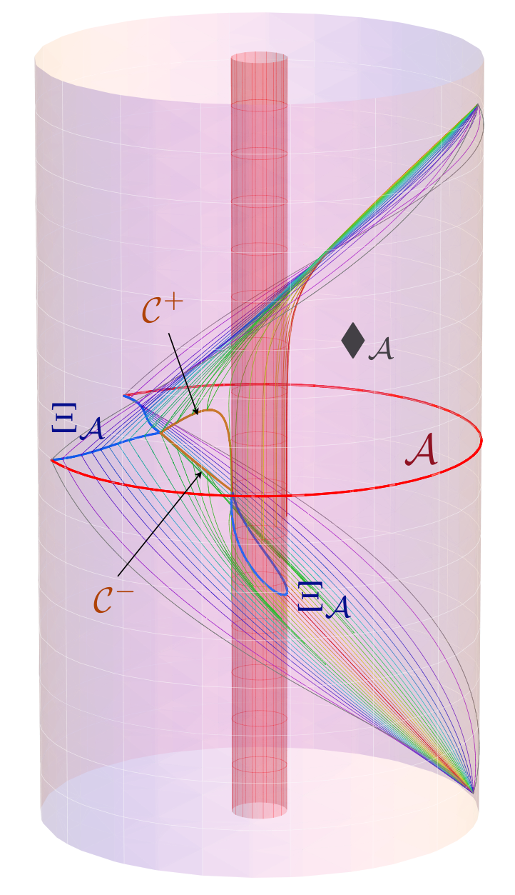
To understand better what happens in the disconnected case, it is instructive to consider the full causal wedge. This is illustrated in Fig. 3 where we plot the causal wedge for the same set of parameters as in the right panel of Fig. 2, but now on a 3-d spacetime diagram in ingoing Eddington coordinates.¹³¹³ 13 Following previous convention [20], we plot $\rho$ radially and choose the vertical coordinate such that ingoing radial null geodesics lie at 45^∘. This fixes the vertical coordinate to be given by $v-\rho+\frac{\pi}{2}$, where $$v=t+\frac{1}{2r_{h}^{2}+1}\left(\sqrt{r_{h}^{2}+1}\,\left[\tan^{-1}\frac{\tan\rho}{\sqrt{r_{h}^{2}+1}}-\frac{\pi}{2}\right]-r_{h}\,\tanh^{-1}\frac{r_{h}}{\tan\rho}\right)\ .$$ For this reason, the plot is asymmetric under vertical flip. There are several features of note: as expected, the causal wedge clearly has a hole, causing $\Xi_{\cal A}$ to have two disconnected components, one anchored on $\partial{\cal A}$ and one wrapping the black hole. This was already necessitated by the observation that the causal wedge cannot penetrate the black hole, while approximating the pure AdS causal wedge far away from the black hole. However, unlike the pure AdS case, the boundary of the causal wedge has caustics where the $L$ and $R$ geodesics from the same congruence intersect each other (before intersecting those from the other congruence). The two caustic curves (${\cal C}^{+}$ on $\partial_{+}(\blacklozenge_{{\cal A}})$ and ${\cal C}^{-}$ on $\partial_{-}(\blacklozenge_{{\cal A}})$) lie at $\varphi=\pi$ and connect the two components of $\Xi_{\cal A}$, where the latter cusps.

As an aside, we remark that the presence of caustics in the causal wedge implies that generically the causal information surface $\Xi_{\cal A}$ need not be smooth; for less symmetric spacetimes this can happen even when $\Xi_{\cal A}$ is connected. Although that might seem like a bizarre feature, it is worth remembering that it is actually no worse than the analogous property of an event horizon, which likewise is not smooth generically.¹⁴¹⁴ 14 Event horizons are locally Lipschitz, but not necessarily more regular than that [27]. There even exist (rather exotic) examples [28] where the event horizon is ‘nowhere’ differentiable, in the sense of non-existence of any open neighbourhood where the horizon is differentiable, though they are differentiable ‘almost everywhere’ in a measure-theoretic sense. More generally, [29] showed that differentiability fails precisely where new generators join the horizons. In particular, although a horizon generator has to remain on the horizon, new generators can enter the horizon at caustics.

Let us now return to considering the effect of varying the parameters, namely the transition between connected and disconnected $\Xi_{\cal A}$ exemplified in Fig. 2. As we decrease the black hole size $r_{h}$ (for a fixed $\varphi_{{\cal A}}$), the curve $\varphi_{t=0}(\ell)$ reaches higher and higher, eventually exceeding $\pi$ (and growing without bound as $r_{h}\to 0$). This is because the null geodesics whose angular momentum is close to $\ell_{0}$ orbit around the black hole many ($\sim r_{h}^{-1}$) times before reaching $t=0$. Conversely, for fixed $r_{h}$, the causal information surface $\Xi_{\cal A}$ is connected if $\varphi_{{\cal A}}$ is sufficiently small (and is guaranteed to be so if $\varphi_{{\cal A}}<\pi/2$ for any $r_{h}$) and disconnected if $\varphi_{{\cal A}}$ is large enough (and is guaranteed to be so when $\varphi_{{\cal A}}\to\pi$ for any $r_{h}$).

This is illustrated in Fig. 4, which plots the causal information surfaces $\Xi_{\cal A}$ for the full range of $\varphi_{{\cal A}}$ at a fixed black hole size ($r_{h}=0.2$, as in Fig. 3), projected onto the Poincaré disk. This presents a somewhat complementary information to that in Fig. 2: whereas the latter varied $r_{h}$ at fixed $\varphi_{{\cal A}}$, Fig. 4 varies $\varphi_{{\cal A}}$ at fixed $r_{h}$.

Since $\varphi_{{\cal A}}$ is connected for small $\varphi_{{\cal A}}$ and disconnected for sufficiently large $\varphi_{{\cal A}}$, we’re guaranteed by continuity that for any $r_{h}$, there is a critical region size $\varphi^{\ast}_{{\cal A}}$ for which $\Xi$ just pinches off. Let us denote the angular momentum along the corresponding null geodesic (i.e. the one passing through this pinch-off point) by $\ell_{\ast}$. The four geodesics, $PR_{\ell_{\ast}}$, $PL_{\ell_{\ast}}$, $FR_{\ell_{\ast}}$, and $FL_{\ell_{\ast}}$, all intersect at a single point $t=0,\varphi=\pi$, and $\rho=\rho_{\ast}$. While this is true whenever $\varphi_{t=0}(\ell)=\pi$, here we have an extra condition that $\Xi_{\cal A}$ self-intersects at a tangent, i.e. that $\max_{\ell\in(0,1)}\varphi_{t=0}(\ell)=\pi$. This condition is satisfied only for a specific relation between $r_{h}$ and $\varphi_{{\cal A}}$. Hence to determine $\ell_{\ast}$ and $\rho_{\ast}$, and correspondingly the critical curve in $(r_{h},\varphi_{{\cal A}})$ plane, we need to be able to find $\max_{\ell\in(0,1)}\varphi_{t=0}(\ell)$ efficiently.

While doing this numerically is rather time-consuming, we can simplify matters using the following observation. Geodesics with angular momentum $\ell_{0}$, when close to $\rho\approx\rho_{0}$, move very slowly in the $\rho$ direction. Hence to compensate, i.e. to remain null, they have to move faster in the $\varphi$ direction to cross the same temporal distance than nearby-$\ell$ geodesics (which move at finite speed in the $\rho$ direction everywhere). Assuming that this effect dominates over what happens to the geodesics in passage between the boundary and vicinity of $\rho_{0}(\ell_{0})$, the $\ell_{0}$ geodesic will reach $\varphi=\pi$ ‘earlier’ than the nearby-$\ell$ geodesics. This in turn means that if we cut them off at $t=0$ to find $\Xi_{\cal A}$, the pinch-off which happens at $\varphi=\pi$ will occur near the $\ell_{0}$ geodesic. This implies that $\ell_{\ast}\approx\ell_{0}$. Assuming that in fact $\ell_{\ast}=\ell_{0}$, it is very simple to find the critical curve in $(r_{h},\varphi_{{\cal A}})$ plane given by a function $\varphi_{{\cal A}}^{\ast}(r_{h})$, since for each fixed $r_{h}$ (which determines $\ell_{0}$ using (2.5)), we merely need to find $\rho_{\ast}$ by solving $t_{\ell_{0}}(\rho_{\ast})=0$, and then integrating the $\ell_{0}$-geodesic from $(t=0,\rho=\rho_{\ast},\varphi=\pi)$ back out to the boundary to find $\varphi_{{\cal A}}$.

We have used this trick to plot the critical curve on $(\varphi_{{\cal A}},\rho_{h})$ plane in Fig. 5 for various spacetime dimensions. The approximation $\ell_{*}\approx\ell_{0}$ can independently be checked by explicit numerical integration and it works extremely well for a large range of black hole sizes.¹⁵¹⁵ 15 In examples that we have examined we find that $\ell_{*}-\ell_{0}\sim 10^{-3}$ for black holes which are roughly of the order of the AdS radius. As expected, for tiny black holes $\rho_{h}\ll 1$, the critical size of the region is $\varphi_{{\cal A}}^{\ast}\to\pi/2$ and grows linearly with $\rho_{h}\sim r_{h}$ since there is effectively no other scale in this regime, whereas for very large black holes $\rho_{h}\gg 1$, $\varphi_{{\cal A}}^{\ast}\to\pi$ asymptoting to a constant. Note that as $\varphi_{{\cal A}}\to\pi$ we are guaranteed to have a non-trivial topology of ${\Xi}_{\cal A}$. In particular, consider the limiting case where ${\cal A}={\bf S^{3}}\backslash i^{0}$, i.e., ${\cal A}$ is a punctured sphere (henceforth denoted as $\varphi_{{\cal A}}=\pi^{-}$). Then no matter how large the black hole is, the causal wedge reaches all the way around the boundary while having a hole due to the horizon. However, from the observation of footnote 8 (further discussed in §3) it follows that the limit $\varphi_{{\cal A}}\to\pi$ is not smooth.

It is worth remarking that the non-trivial topology of the causal wedge described above relies on working in global Schwarzschild-AdS geometry. In the planar Schwarzschild-AdS black hole geometry, one cannot circumnavigate the black hole, there being no “other side”. Nevertheless, as we will describe later, even in the Poincaré patch of AdS it is possible to encounter causal wedges with non-trivial topology; for instance a localized black hole in the Poincaré patch will likewise do the trick (see §2.3).

Above we have presented an example of a causal wedge with one hole. It is now conceptually easy to generalize this situation to a causal wedge with multiple holes. For example, we can consider a (dynamical) situation with multiple small black holes in AdS.¹⁶¹⁶ 16 While such solutions are not known analytically one can construct approximate solutions using a matched asymptotics method. The black holes will generically orbit each other on timescales set by their separation, radiate gravitational waves, and eventually coalesce. But we can separate scales in such a way that around each black hole there is a region which is inside a causal wedge for appropriate ${\cal A}$. In fact, if $\varphi_{{\cal A}}\approx\pi/2$, we may see transitions in the number of components of $\Xi$. For small black holes and $\varphi_{{\cal A}}$ larger than $\pi/2$ by amount related to the black hole separation, $\Xi_{\cal A}$ will have a component around each horizon, apart from the one connected to $\partial{\cal A}$. Hence for a ‘galaxy’ with $N$ separated black holes in AdS, $\Xi$ will have $N+1$ disconnected components.

So far, this section has focused on the topology of the causal wedge and the connectedness of $\Xi_{\cal A}$. Before closing, let us make an observation about the nature of the ‘phase transition’ between connected and disconnected $\Xi_{\cal A}$ as seen by its area $\chi_{\cal A}$. Although we don’t evaluate the causal holographic information $\chi$ explicitly, we expect that for fixed $r_{h}$, $\chi_{\cal A}(\varphi_{{\cal A}})$ is not smooth at the transition point $\varphi^{\ast}_{{\cal A}}$. Consider the full curve (on our $(t,\rho,\varphi)$ subspace) ${\cal X}_{t=0}$ generated by intersections of future and past geodesics, characterized by $(\rho_{t=0}(\ell),\varphi_{t=0}(\ell))$. The causal information surface $\Xi_{\cal A}$ is a subset of this curve, restricted by $\varphi_{t=0}(\ell)\leq\pi$; in particular the two curves are identical only when $\Xi_{\cal A}$ has just one connected component. Since the spacetime is smooth, the geodesics, and hence their intersections, must vary smoothly in $\ell$. Similarly, the length of the full ${\cal X}_{t=0}$ should vary smoothly as we change $\varphi_{{\cal A}}$. However, at the transition point $\varphi^{\ast}_{{\cal A}}$, $\chi$ ceases to be given by length of ${\cal X}_{t=0}$: the difference is given by the finite length piece where $\varphi_{t=0}(\ell)>\pi$. We would therefore expect that $\chi_{\cal A}(\varphi_{{\cal A}})$ has a kink at $\varphi_{{\cal A}}=\varphi^{\ast}_{{\cal A}}$.

Having seen the rich structure of $\Xi_{\cal A}$ for Schwarzschild-AdS₅, one might wonder whether it is also present in the simpler case of the 3-dimensional BTZ geometry, which has the form (2.2) with

Here the calculation is in fact much simpler, and the explicit expressions for null geodesics which generate $\partial\blacklozenge_{{\cal A}}$ were presented in e.g. [20]. A representative causal wedge is plotted in the left panel of Fig. 6. We choose $\varphi_{{\cal A}}=2.5$ as in Fig. 3, and we use a tiny black hole $r_{h}=0.02$ in order to emphasize the difference from the higher-dimensional case.

In fact, as observed already in [13], in BTZ spacetime $\Xi_{\cal A}$ exactly coincides with ${\mathfrak{E}}_{{\cal A}}$; the latter corresponds to the spacelike geodesic anchored at $\pm\varphi_{{\cal A}}$ on the boundary. The spatial projection of these is described by

As can be easily seen, connected spacelike geodesics always exist for arbitrary $\varphi_{{\cal A}}$, as illustrated in the right panel of Fig. 6.

One reason why the causal wedge does not close off as in the higher dimensional case is that taking the black hole arbitrarily small $r_{h}\to 0$ does not approach pure AdS: the latter is achieved when $r_{h}^{2}=-1$. Said differently, in 3 dimensions, the influence of the black hole does not fall off fast enough. Not only are the effects of a tiny BTZ black hole perceptible on AdS scale, but even near the boundary there is a qualitative difference between presence and absence of a black hole. A different way to see that 3-dimensional bulk is special is to note that we have argued that causal wedges must be simply connected to the boundary domain ${\cal A}$ [19] as follows form topological censorship [23]. Since in this low dimension ${\Xi}_{\cal A}$ is a curve, it must be smoothly deformable to $\Diamond_{\cal A}$. It thus follows that there is no room for non-trivial topology of ${\Xi}_{\cal A}$ in three dimensional bulk spacetimes.

In §2.1 we have seen that for higher dimensional Schwarzschild-AdS black hole of any size, the causal wedge has holes for sufficiently large boundary region ${\cal A}$. As $r_{h}\to\infty$, the critical size of ${\cal A}$ for which $\Xi_{\cal A}$ becomes disconnected approaches $\varphi_{{\cal A}}^{\ast}\to\pi$, whereas for $r_{h}\to 0$, the critical size $\varphi_{{\cal A}}^{\ast}\to\pi/2$. In particular, to obtain disconnected $\Xi_{\cal A}$ for this class of geometries, the region ${\cal A}$ must cover at least half of the boundary sphere, and therefore sample a large part of the system. However, we now argue that large ${\cal A}$ is actually not a prerequisite for existence of disconnected $\Xi_{\cal A}$, in the sense that for any finite region ${\cal A}$ on the boundary we can construct asymptotically AdS geometries (in more than 3 dimensions) for which $\Xi_{\cal A}$ is disconnected.

In fact, a simple example which does the job is a boosted version of the global Schwarzschild-AdS black hole discussed in §2.1. We can consider a family of geometries, considered e.g. in [1], corresponding to a boosted global black hole with fixed total energy.¹⁷¹⁷ 17 See also [30] for a recent discussion where such geometries were called oscillons. At zero boost this is the standard global AdS black hole while at infinite boost, this solution limits to a gravitational shock wave in AdS. In the static coordinates (defined with respect to a specified boundary time), the boosted black hole follows a trajectory which approximates that of a timelike geodesic.

We don’t need to do a new calculation to see what will happen for causal wedges in such a geometry, since we can simply boost our causal wedge for the static black hole found in §2.1. In other words, we can implement a coordinate transformation which in pure AdS would transform a timelike geodesic at the origin $\rho(t)=0$ to one which oscillates back and forth with energy $E>1$, whose radial profile is given by

The requisite transformation is most easily obtained from isometrically embedding AdS_d+1 into ${\mathbf{R}}^{d,2}$ endowed with the flat metric $ds^{2}=-dX_{-1}^{2}-dX_{0}^{2}+\sum_{i=1}^{d}dX_{i}^{2}$, restricted to the hyperboloid $-X_{-1}^{2}-X_{0}^{2}+\sum_{i=1}^{d}X_{i}^{2}=-1$. This embedding makes the AdS isometries obvious: for instance we have manifest boost invariance, say $X_{0}\to\cosh\beta\,X_{0}+\sinh\beta\,X_{1}$ and $X_{1}\to\cosh\beta\,X_{1}+\sinh\beta\,X_{0}$, leaving all the other $X_{i}$’s unchanged. The energy $E$ in (2.13) is related to the boost in the obvious manner $E=\cosh\beta$. So the relevant isometric embedding, which implements the boost and yields AdS in the conformally ESU coordinates, i.e. (2.2) with $g(\rho)=1$, is

where $\Omega_{i}$ with $i=2,\cdots,d$ are direction cosines, i.e., $\sum_{i}\,\Omega_{i}^{2}=1$, coordinatizing a unit ${\bf S}^{d-2}$ and thus explicitly ensuring the $SO(d-1)$ symmetry in the transverse space. The actual transformation is then generated by comparing the $X$’s for $\beta=0$ with those for arbitrary boost in (2.14), and is given (modulo some branch issues) by

where the barred coordinates correspond to boost with respect to the unbarred coordinates by a boost $\beta$. The direction cosines are unchanged since we retain $SO(d-1)$ symmetry.

Note that the boundary is preserved, ${\bar{\rho}}(\rho=\frac{\pi}{2},t,\varphi)=\frac{\pi}{2}$ under (2.15), and this then specifies the corresponding transformation induced on the boundary. More precisely, the bulk coordinate transform implementing the boost corresponds to a conformal transformation (involving both time and space) on the boundary. This transformation changes the size of $\Diamond_{\cal A}$. In particular, small ${\cal A}$ and highly boosted black hole translates to large ${\cal A}$ in the static black hole frame, at time where the black hole is closest to the region ${\cal A}$ on the boundary in the boosted picture.

This is illustrated in Fig. 7, which shows how a fixed size region ${\cal A}$ taken at different times translates into a variable-sized region in a boosted frame with relative boost $\beta$ (red curve corresponds to zero boost while purple to $\beta=4$). If we take a hemispherical region with ${\bar{\varphi}}_{\cal A}=\pi/2$ (left), the ‘breathing’ of its size $\varphi_{{\cal A}}$ in the boosted frame is symmetric, whereas starting with a small region (right) only produces large sizes in the boosted frame at short intervals. Nevertheless, it is easy to see that no matter how small we take the region ${\cal A}$ in the unboosted frame, its size in the boosted frame can get arbitrarily close to $\pi$ for sufficiently large boosts.

It is now a simple matter to translate the effect of the boost on the causal wedge: it is precisely the same effect as that of varying the size of $\varphi_{{\cal A}}$. The topological attributes cannot change by the coordinate transformation; so since $\blacklozenge_{{\cal A}}$ has a hole in unboosted frame (equivalently the static black hole spacetime) for large regions, the same is true in the boosted frame (equivalently in the boosted black hole spacetime) even for small regions – but only at the auspicious times and for sufficient boosts.

It is worth noting that another construction which describes the same (Schwarzschild-AdS) geometry in different coordinates is obtained by simply restricting attention to the Poincaré patch of global Schwarzschild-AdS. The CFT dual on Minkowski space of such configurations was dubbed ‘the conformal soliton flow’ by [24]. The event horizon defined with respect to the Poincaré patch is then closely analogous to the boundary of the causal wedge, since it is generated by null geodesics in Schwarzschild-AdS which end on the boundary at $i^{+}$ of the Poincaré patch which corresponds to some finite ESU time; this was constructed explicitly in [31] (cf., their Figure 3 for a plot¹⁸¹⁸ 18 Strictly speaking the plot in [31] is for the BTZ conformal soliton where we have argued for the absence of non-trivial topology; a similar picture in higher dimensions should reveal the appropriate structure. of the event horizon in global coordinates in 3 dimensions, though the vertical axis is the BTZ time $t$ rather than the coordinate used above in Fig. 6 which is more analogous to Eddington time). More precisely, the future event horizon indicated there would correspond to $\partial_{+}(\blacklozenge_{{\cal A}})$ for $\varphi_{{\cal A}}=\pi$, though $\Xi_{\cal A}$ for any other $\varphi_{{\cal A}}$ can easily be read off by slicing their blue surface horizontally higher than $i^{0}$.

So far in this subsection we have discussed geometries which are static though not manifestly so (they all admit a Killing field which is timelike everywhere outside of event horizon). It is even easier to construct examples with disconnected $\Xi_{\cal A}$ for dynamical situations with collapsing and evaporating black holes, where the event horizon lasts only for a finite time. Again by separation of scales, if the black holes are tiny on AdS scale we can put them anywhere, and they will only eat out tiny spacetime regions from the AdS causal wedge. Then the original $\partial\blacklozenge_{{\cal A}}$ (connected to $\partial\Diamond_{\cal A}$) will be only minimally deformed but the full $\partial\blacklozenge_{{\cal A}}$ will now include additional disconnected components. This will again translate into $\Xi_{\cal A}$ having multiple components, but now if we try to project them onto a single Poincaré disk, they may even intersect. However, topological censorship will still guarantee that the causal wedge remains simply connected.

Finally, note that since we can take ${\cal A}$ arbitrarily small, the above construction can likewise be implemented in Poincaré AdS, where the dual CFT lives on flat space. In other words, having asymptotically global AdS bulk geometry is not a prerequisite to disconnected $\Xi_{\cal A}$ either.

So far all our examples of disconnected $\Xi_{\cal A}$ involved causally non-trivial bulk geometries. In such situations it is easy to argue from first principles that for sufficiently large ${\cal A}$ the causal wedge must have holes, since by causality $\blacklozenge_{{\cal A}}$ cannot reach past the event horizon. However, we will now see that the presence of an event horizon is not a prerequisite for disconnected $\Xi_{\cal A}$. As long as ${\cal A}^{c}\neq\emptyset$ and we are in more than 3 bulk dimensions, all of the examples discussed above can be modified to keep the geometry causally trivial but nevertheless the causal wedge unaffected. In black hole geometries, null geodesics starting arbitrarily near the event horizon take a long time to reach the AdS boundary. So they typically don’t make it out to $\Diamond_{\cal A}$; as a result $\Xi_{\cal A}$ remains a finite distance away from the event horizon.¹⁹¹⁹ 19 This is an extreme case of the time delay effect discussed in [3]. We could then take the metric to remain identical in the region reached by $\blacklozenge_{{\cal A}}$ but modify it outside that region so as to get rid of all the horizons.

For example in the Schwarzschild-AdS case, we could in principle replace the black hole by a compact star (or even a static shell) which is just slightly bigger than the original black hole. To find out whether or not this is physically realistic, let us examine how compact would such a star have to be. Since its maximal size is bounded by the deepest reach of $\Xi_{\cal A}$, and the latter occurs at $\varphi=0$, we merely need to see how deep does the radial ($\ell=0$) null geodesic from ${q^{\vee}}$ penetrate by the time $t=0$. This value of course depends on both $\varphi_{{\cal A}}$ and $r_{h}$. When $\varphi_{{\cal A}}$ is small, the geodesic of course does not have time to reach very deep, but then the causal wedge does not have holes, so this regime is irrelevant for our purposes. On the other hand, if we take $\varphi_{{\cal A}}$ too large in order to guarantee $\blacklozenge_{{\cal A}}$ having a hole, the geodesics have longer time to travel and typically they approach exponentially close to the horizon. For example in the case illustrated in Fig. 3, the $\rho$ value reached by the radial (red) geodesics $\rho_{\Xi}$ is already very close to the horizon: $\frac{\rho_{\Xi}-\rho_{h}}{\rho_{h}}\approx 5\times 10^{-6}$, which is scarcely realistic for a compact star.

To maximize the size of the requisite star, then, we want to minimize $\varphi_{{\cal A}}$ subject to $\Xi_{\cal A}$ being disconnected, i.e. take $\varphi_{{\cal A}}=\varphi_{{\cal A}}^{\ast}$, and study the corresponding $\rho_{\Xi}$ as a function of $\rho_{h}$. Numerical studies indicate that the maximal value attained, which occurs in the limit of tiny black holes, is $\frac{\rho_{\Xi}-\rho_{h}}{\rho_{h}}\approx 10^{-4}$. While this is still not be achievable for physically relevant equations of state for the star, it demonstrates the matter-of-principle point that event horizons are not necessary for topologically non-trivial causal wedge. In fact, preliminary investigations indicate that it might be possible for charged scalar solitons in AdS to have non-trivial causal wedge topology; it would be interesting to explore this further.

The simple properties which we prove in §3.2 are as follows:

1. (1).

   If ${\cal A}_{t}\cap{\cal B}_{t}=\emptyset$ (and more generally if ${\cal{A}}$ and ${\cal{B}}$ are spacelike-separated), then $\blacklozenge_{{\cal A}}$ and $\blacklozenge_{{\cal B}}$ are spacelike-separated. Hence $\blacklozenge_{{\cal A}}\cap\blacklozenge_{{\cal B}}=\emptyset$ and $\Xi_{\cal A}$ and $\Xi_{\cal B}$ are likewise spacelike-separated.

2. (2).

   If ${\cal A}_{t}\subset{\cal B}_{t}$ (and more generally if $\Diamond_{\cal A}\subset\Diamond_{{\cal B}}$), then $\blacklozenge_{{\cal A}}\subset\blacklozenge_{{\cal B}}$.
   Moreover, if ${\cal A}_{t}$ is entirely inside ${\cal B}_{t}$ (more generally if $\partial\Diamond_{\cal A}\cap\partial\Diamond_{{\cal B}}=\emptyset$), then $\Xi_{\cal A}$ and $\Xi_{\cal B}$ are spacelike-separated, with $\Xi_{{\cal B}}$ lying deeper than $\Xi_{{\cal A}}$ (equivalently outside $\blacklozenge_{{\cal A}}$).

3. (3).

   If ${\cal A}_{t}$ and ${\cal B}_{t}$ overlap (i.e., if ${\cal A}\cap{\cal B}\neq\emptyset$, but ${\cal A}\backslash{\cal B}\neq\emptyset$ and ${\cal B}\backslash{\cal A}\neq\emptyset$), then

   $$\blacklozenge_{{\cal A}\cap{\cal B}}\subset\blacklozenge_{{\cal A}}\cap\blacklozenge_{{\cal B}}\subset\big\{\blacklozenge_{{\cal A}},\blacklozenge_{{\cal B}}\big\}\subset\blacklozenge_{{\cal A}}\cup\blacklozenge_{{\cal B}}\subset\blacklozenge_{{\cal A}\cup{\cal B}}\ .$$

   (3.1)

   where by $\big\{\blacklozenge_{{\cal A}},\blacklozenge_{{\cal B}}\big\}$ we mean either $\blacklozenge_{{\cal A}}$ or $\blacklozenge_{{\cal B}}$. Moreover, $\Xi_{{\cal A}\cup{\cal B}}$ and $\Xi_{{\cal A}\cap{\cal B}}$ are spacelike-separated, with $\Xi_{{\cal A}\cup{\cal B}}$ lying deeper than $\Xi_{{\cal A}\cap{\cal B}}$ (i.e. outside $\blacklozenge_{{\cal A}\cap{\cal B}}$), etc.

4. (4).

   For any (not necessarily stationary) bulk black hole spacetimes, no causal wedge can penetrate the event horizon. It then immediately follows that $\Xi_{\cal A}$ cannot penetrate an event horizon for any ${\cal A}$.

5. (5).

   Causal holographic information satisfies Additivity:
   If ${\cal A}\cap{\cal B}=\emptyset$, then $\chi_{{\cal A}\cup{\cal B}}=\chi_{{\cal A}}+\chi_{{\cal B}}$.

6. (6).

   Causal holographic information satisfies Subadditivity:
   If ${\cal A}\cap{\cal B}\neq\emptyset$, then $\chi_{{\cal A}\cup{\cal B}}\leq\chi_{\cal A}+\chi_{\cal B}$.
   (However, Strong Subadditivity is not necessarily satisfied, as demonstrated in [13].)

7. (7).

   From the set of all surfaces on $\partial\blacklozenge_{{\cal A}}$ anchored on $\partial{\cal A}$, $\Xi_{\cal A}$ is the minimal-area one.

8. (8).

   Extremal surface ${\mathfrak{E}}_{\cal A}$ must lie outside (or on the boundary of) the causal wedge $\blacklozenge_{{\cal A}}$.²¹²¹ 21 However, as demonstrated in [20], ${\mathfrak{E}}_{\cal A}$ and $\Xi_{\cal A}$ need not be always spacelike-separated. When they are, the above statement guarantees that ${\mathfrak{E}}_{\cal A}$ lies deeper than $\Xi_{\cal A}$.

Some of the proofs of the above statements use the concept of a causal curve, which we take to be a nowhere-spacelike, maximally extended, connected curve (either in the bulk or along the boundary). We will denote a future-directed causal curve from a point $p$ to a point $q$ in the spacetime by $\gamma_{p\to q}^{+}=\gamma_{q\to p}^{-}$. Existence of such a curve guarantees that $q$ is in the future of $p$.