Minimum Degree of the Difference of Two Polynomials over ${\mathbb{Q}}$ , and Weighted Plane Trees.

Fedor Pakovich ^†^†thanks: Department of Mathematics, Faculty of Natural Sciences, Ben-Gurion University of the Negev, P.O.B. 653, Beer Sheva, Israel; pakovich@math.bgu.ac.il. and Alexander K. Zvonkin ^†^†thanks: LaBRI, Université Bordeaux I, 351 cours de la Libération, F-33405 Talence Cedex France; zvonkin@labri.fr.

August 24, 2026

Abstract

A weighted bicolored plane tree (or just tree for short) is a bicolored plane tree whose edges are endowed with positive integral weights. The degree of a vertex is defined as the sum of the weights of the edges incident to this vertex. Using the theory of dessins d’enfants, which studies the action of the absolute Galois group on graphs embedded into Riemann surfaces, we show that a weighted plane tree is a graphical representation of a pair of coprime polynomials $P,Q\in{\mathbb{C}}\,[x]$ such that: (a) $\deg P=\deg Q$ , and $P$ and $Q$ have the same leading coefficient; (b) the multiplicities of the roots of $P$ (respectively, of $Q$ ) are equal to the degrees of the black (respectively, white) vertices of the corresponding tree; (c) the degree of the difference $P-Q$ attains the minimum which is possible for the given multiplicities of the roots of $P$ and $Q$ . Moreover, if a tree in question is uniquely determined by the set of its black and white vertex degrees (we call such trees unitrees), then the corresponding polynomials are defined over ${\mathbb{Q}}$ .

The pairs of polynomials $P,Q$ such that the degree of the difference $P-Q$ attains the minimum, and especially those defined over ${\mathbb{Q}}$ , are related to some important questions of number theory. Dozens of papers, from 1965 [4] to 2010 [3], were dedicated to their study. The main result of this paper is a complete classification of the unitrees which provides us with the most massive class of such pairs defined over ${\mathbb{Q}}$ . We also study combinatorial invariants of the Galois action on trees, as well as on the corresponding polynomial pairs, which permit us to find yet more examples defined over ${\mathbb{Q}}$ . In a subsequent paper we compute the polynomials $P,Q$ corresponding to all the unitrees.

1 Introduction

In 1965, Birch, Chowla, Hall, and Schinzel [4] asked a question which soon became famous:

Let $A$ and $B$ be two coprime polynomials with complex coefficients; what is the possible minimum degree of the difference $R=A^{3}-B^{2}$ ?

It is reasonable to suppose that $A^{3}$ and $B^{2}$ have the same degree and the same leading coefficients. Let us take $\deg A=2k$ , $\deg B=3k$ , so that $\deg A^{3}=\deg B^{2}=6k$ . Then the following was conjectured in [4]:

1.

For $R=A^{3}-B^{2}$ one always has $\deg R\geq k+1$ .
2.

This bound is sharp: that is, it is attained for infinitely many values of $k$ .

The first conjecture was proved the same year by Davenport [8]. The second one turned out to be much more difficult and remained open for 16 years: in 1981 Stothers [24] showed that the bound is in fact attained not only for infinitely many values of $k$ but for all of them.

The above problem may be generalized in various ways. The following one was considered in 1995 by Zannier [26]. Let $\alpha,\beta\vdash n$ be two partitions of $n$ ,

\alpha=(\alpha_{1},\ldots,\alpha_{p}),\quad\beta=(\beta_{1},\ldots,\beta_{q}),\quad\sum_{i=1}^{p}\alpha_{i}=\sum_{j=1}^{q}\beta_{j}=n,

and let $P$ and $Q$ be two coprime polynomials of degree $n$ having the following factorization pattern:

\displaystyle P(x)\,=\,\prod_{i=1}^{p}\,(x-a_{i})^{\alpha_{i}}\,,\qquad Q(x)\,=\,\prod_{j=1}^{q}\,(x-b_{j})^{\beta_{j}}\,.

(1)

In these expressions we consider the multiplicities $\alpha_{i}$ and $\beta_{j}$ , $i=1,2,\ldots,p$ , $j=1,2,\ldots,q$ as being given, while the roots $a_{i}$ and $b_{j}$ are not fixed, though they must all be distinct. The problem is to find the minimum possible degree of the difference $R=P-Q$ . In his paper, Zannier proved the following. Let $d={\rm gcd}\,(\alpha,\beta)$ denote the greatest common divisor of the numbers $\alpha_{1},\ldots,\alpha_{p},\beta_{1},\ldots,\beta_{q}$ . If

\displaystyle p+q\,\leq\,\frac{n}{d}+1

(2)

then

\displaystyle\deg R\,\geq\,(n+1)-(p+q),

(3)

and this bound is always attained. If, on the other hand, $p+q>\frac{n}{d}+1$ , then a weaker bound

\displaystyle\deg R\,\geq\,\frac{(d-1)\,n}{d},

(4)

is valid, and it is also attained.

Definition 1.1 (Davenport–Zannier triple)

Let $P,Q,R\in{\mathbb{C}}\,[x]$ be coprime polynomials with factorization pattern (1), $\deg P=\deg Q=n$ , while the degree of the polynomial $R=P-Q$ equals $(n+1)-(p+q)$ . Then the triple $(P,Q,R)$ is called a Davenport–Zannier triple, or, in a more concise way, a DZ-triple.

The main subject of this paper is a study of DZ-triples defined over ${\mathbb{Q}}$ , that is, the triples $P,Q,R\in{\mathbb{Q}}\,[x]$ .

The paper is organized as follows.

A preliminary work is carried out in Section 2. First, we show that bound (3) follows from the Riemann–Hurwitz formula for the function $f=P/R$ . Then we reduce the problem about polynomials to a problem about weighted bicolored plane trees. A weighted bicolored plane tree is a plane tree (“plane” means that the cyclic order of branches around each vertex is fixed) whose vertices are colored in black and white in such a way that the ends of each edge have opposite colors, and whose edges are endowed with positive integral weights. The degree of a vertex is defined as the sum of the weights of the edges incident to this vertex. The sum of the weights of all the edges is called the total weight of the tree. We show that a DZ-triple with prescribed factorization pattern (1) exists if and only if there exists a weighted bicolored plane tree of the total weight $n=\deg P=\deg Q$ having $p$ black vertices of degrees $\alpha_{1},\ldots,\alpha_{p}$ and $q$ white vertices of degrees $\beta_{1},\ldots,\beta_{q}$ . As a corollary, we give a spectacularly simple proof of Stothers’s 1981 result for the squares and cubes, namely, the attainability of the lower bound $\deg(A^{3}-B^{2})\geq k+1$ where $\deg A=2k$ and $\deg B=3k$ , see Example 2.13. The results of Section 2 as well as the framework of the whole paper are based on the theory of dessins d’enfants (see, e. g., Chapter 2 of [17], or a collection of papers [22], or a recent book [11]). This theory establishes a correspondence between simple combinatorial objects, graphs drawn on two-dimensional surfaces, and a vast world of Riemann surfaces, algebraic curves, number fields, Galois theory, etc.

In Section 3 we prove the existence theorem for weighted bicolored plane trees. Namely, we show that a necessary and sufficient condition for the existence of a tree with the above characteristics is inequality (2). The attainability of bound (3) is deduced from this result. In Section 4 we establish bound (4) and its attainability in the case when inequality (2) is not satisfied. Although bounds (3) and (4) and their attainability were proved by U. Zannier, we reprove these results here for the sake of completeness, and also in order to show how the pictorial language clarifies and simplifies the exposition.

In Sections 5 and 6 we study DZ-triples defined over ${\mathbb{Q}}$ . This case is the most interesting one since by specializing $x$ to a rational value one may obtain an important information concerning differences of integers with given factorization patterns. This subject is actively studied in number-theoretic works: see, for example, a recent paper by Beukers and Stewart [3] (2010) and the bibliography therein. Our approach here is based on the following corollary of the theory of dessins d’enfants which gives a sufficient (though not necessary) condition for a DZ-triple to be defined over ${\mathbb{Q}}$ : the triple is defined over ${\mathbb{Q}}$ if there exists exactly one weighted bicolored plane tree with the degrees of black vertices equal to $\alpha_{1},\ldots,\alpha_{p}$ , and the degrees of white vertices equal to $\beta_{1},\ldots,\beta_{q}$ . We will call such trees unitrees.

In Section 5 we prove the main result of the paper, namely, a complete classification of unitrees: see Theorem 5.4. The formulation of this theorem is rather long so we do not enunciate it in the Introduction. We mention only that the class of unitrees consists of ten infinite series of trees and ten sporadic trees which do not belong to the above series.

While the results of Section 5 may be considered as conclusive, Section 6 represents only first steps in a far-ranging programme of study of the Galois action on weighted plane trees and of combinatorial invariants of this action. This approach permits to find yet more DZ-triples defined over ${\mathbb{Q}}$ and also to study DZ-triples over other number fields. Note that essentially all previously found examples of DZ-triples over ${\mathbb{Q}}$ correspond either to unitrees or to the trees constructed in Section 6. We have also found quite a few new examples of DZ-triples.

Finally, in Section 7 we mention some further possible developments of the subject.

This paper deals only with the combinatorial aspect of the whole construction. The computation of the corresponding DZ-triples is postponed to a separate publication (see [20]) since the techniques used for this purpose are very different form the ones used in this paper. In particular, a great deal of symbolic computations as well as certain polynomial identities are required. For an individual unitree, the computation of the corresponding DZ-triple is a difficult task but the verification of the result is easy. Indeed, when polynomials $P,Q,R$ (together with their appropriate factorizations) are given, it is immediate to observe that their coefficients are rational, and the only thing to verify is that $R$ is indeed equal to $P-Q$ . The situation becomes significantly more complicated for infinite series of trees since in this case the proof may become rather elaborate.

2 From polynomials through Belyi functions to weighted trees

2.1 Function $f=P/R$ and its critical values

Let $\alpha,\beta\vdash n$ be two partitions of $n$ , $\alpha=(\alpha_{1},\ldots,\alpha_{p})$ , $\beta=(\beta_{1},\ldots,\beta_{q})$ , $\sum_{i=1}^{p}\alpha_{i}=\sum_{j=1}^{q}\beta_{j}=n$ , and let $P,Q\in{\mathbb{C}}[x]$ be two polynomials of degree $n$ with the factorizations

\displaystyle P(x)\,=\,\prod_{i=1}^{p}\,(x-a_{i})^{\alpha_{i}}\,,\qquad Q(x)\,=\,\prod_{j=1}^{q}\,(x-b_{j})^{\beta_{j}}\,.

(5)

We suppose all $a_{i},b_{j}$ , $i=1,\ldots,p$ , $j=1,\ldots,q$ to be distinct. Let the difference $R=P-Q$ have the following factorization:

\displaystyle R(x)\,=\,\prod_{k=1}^{r}\,(x-c_{k})^{\gamma_{k}}\,,\qquad\deg R\,=\,\sum_{k=1}^{r}\,\gamma_{k}\,.

(6)

Our goal is to minimize $\deg R$ ; obviously,

\displaystyle\deg R\geq r.

(7)

Consider the following rational function of degree $n$ :

f\,=\,\frac{P}{R}\,;

note that

f-1\,=\,\frac{Q}{R}\,.

Definition 2.1 (Critical value)

A point $y\in\overline{{\mathbb{C}}}={\mathbb{C}}\cup\{\infty\}$ is called critical value of a rational function $f$ if the equation $f(x)=y$ has multiple roots.

The expressions written above for the function $f=P/Q$ provide us with at least three critical values of $f$ :

•

$y=0$ , provided that not all $\alpha_{i}$ are equal to 1;
•

$y=1$ , provided that not all $\beta_{j}$ are equal to 1; and
•

$y=\infty$ , if only we do not consider the trivial case $\deg R=\deg P-1$ ; if $\deg R<\deg P-1$ then $f$ has a multiple pole at infinity.

Denote $y_{1},\ldots,y_{m}$ the other critical values of $f$ , if there are any, and let $n_{l}$ be the number of preimages of $y_{l}$ , $l=1,\ldots,m$ ; by the definition of a critical value, $n_{l}<n$ .

Lemma 2.2 (Number of roots of $R$ )

The number $r$ of distinct roots of the polynomial $R$ is

\displaystyle r\,=\,(n+1)-(p+q)+\sum_{l=1}^{m}\,(n-n_{l}).

(8)

In fact, equality (8) is a particular case of the Riemann–Hurwitz formula, but for the sake of completeness we give its proof here.

Proof.

Let us draw a star-tree with the center at 0 and with its rays going to the critical values $1,y_{1},\ldots,y_{m}$ , see Figure 1. Considered as a map on the sphere, this tree has $m+2$ vertices, $m+1$ edges, and a single outer face with its “center” at $\infty$ .

Refer to caption — Figure 1: Star-tree whose vertices are critical values of $f$ .

Now let us take the preimage of this tree under $f$ . We will get a graph drawn on the preimage sphere which has $n\,(m+1)$ edges since each edge is “repeated” $n$ times in the preimage. Its vertices are the preimages of the points $0,1,y_{1},\ldots,y_{m}$ , so their number is equal to $p+q+\sum_{l=1}^{m}n_{l}$ .

What occurs to the faces?

If we puncture at $\infty$ the single open face in the image sphere, we get a punctured disk without any ramification points inside. The only possible unramified covering of a punctured open disk is a disjoint collection of punctured disks; their number is equal to the number of poles of $f$ , namely, $r+1$ ( $r$ roots of $R$ and $\infty$ ). Inserting a point into each puncture we get $r+1$ simply connected open faces in the preimage sphere. The fact that they are simply connected implies that the graph drawn on the preimage sphere is connected. Thus, the preimage of our star-tree is a plane map. What remains is to apply Euler’s formula:

\left(p+q+\sum_{l=1}^{m}n_{l}\right)-n\,(m+1)+(r+1)\,=\,2,

which leads to (8). $\Box$

Notice that in order to prove Lemma 2.2, instead of the tree of Figure 1, we could take any other plane map with vertices at the critical values (see e.g. the proof of Proposition 4.2 below).

Corollary 2.3 (Lower bound)

We have

\displaystyle\deg R\,\geq\,(n+1)-(p+q)\,.

(9)

The proof follows from (8) and (7). $\Box$

Note that $\deg R$ cannot be negative; therefore, when $p+q>n+1$ the latter bound cannot be attained. In this case one can attain the bound $\deg R\geq 0$ , that is, the polynomial $R$ can be made equal to a constant. This situation is studied in more detail in Section 4.

Equation (8) provides us with guidelines of how to get the minimum degree of $R$ .

Proposition 2.4 (Bound (9) attainability)

Bound (9) is attained if and only if the following conditions are satisfied:

•

$p+q\leq n+1$ .
•

The number $m$ of the critical values of $f$ other than $0,1,\infty$ , is equal to zero, so that the sum $\sum_{l=1}^{m}\,(n-n_{l})$ in the right-hand side of (8) is eliminated altogether. The tree of Figure 1 is then reduced to merely the segment $[0,1]$ .
•

All the roots of $R$ are simple, that is, $\gamma_{1}=\ldots=\gamma_{r}=1$ , so that $\deg R=r$ . Another formulation of the same condition: the partition $\gamma\vdash n$ , $\gamma=(\gamma_{0},\gamma_{1},\gamma_{2},\ldots,\gamma_{r})$ , which corresponds to the multiplicities of the poles, has the form of a hook: $\gamma=(n-r,\underbrace{1,1,\ldots,1}_{r\ \mathrm{times}})=(n-r,1^{r})$ .

The conditions which imply the existence of such a function $f$ will be obtained in Section 3.

2.2 Dessins d’enfants and Belyi functions

Considering rational functions with only three critical values brings us into the framework of the theory of dessins d’enfants. Here we give a brief summary of this theory (only in a planar setting); the missing details, proofs, and bibliography can be found, for example, in [17], Chapter 2.

Definition 2.5 (Belyi function)

A rational function $f:\overline{{\mathbb{C}}}\to\overline{{\mathbb{C}}}$ is called Belyi function if it does not have critical values outside the set $\{0,1,\infty\}$ .

For such a function, the tree considered in the proof of Lemma 2.2 is reduced to the segment $[0,1]$ . Let us take this segment, color the point 0 in black and the point 1 in white, and consider the preimage $D=f^{-1}([0,1])$ ; we will call this preimage a dessin.

Proposition 2.6 (Dessin)

The dessin $D=f^{-1}([0,1])$ is a connected graph drawn on the sphere, and its edges do not intersect outside the vertices. Therefore, $D$ may also be considered as a plane map. This map has a bipartite structure: black vertices are preimages of $0$ , and white vertices are preimages of $1$ .

The degrees of the black vertices are equal to the multiplicities of the roots of the equation $f(x)=0$ , and the degrees of the white ones are equal to the multiplicities of the roots of the equation $f(x)=1$ . The sum of the degrees in both cases is equal to $n=\deg f$ , which is also the number of edges.

The map $D$ being bipartite, the number of edges surrounding each face is even. It is convenient, in defining the face degrees, to divide this number by two.

Definition 2.7 (Face degree)

We say that an edge is incident to a face if, while remaining inside this face and making a circuit of it in the positive (trigonometric) direction, we follow the edge from its black end toward the white one. Thus, only half of the edges surrounding a face are incident to it. Moreover, each edge is incident to exactly one face. The degree of a face is equal to the number of edges incident to it.

According to this definition and to the remarks preceding it, every edge is incident to one black vertex, to one white vertex, and to one face. The sum of the face degrees is equal to $n=\deg f$ .

Proposition 2.8 (Faces and poles)

Inside each face there is a single pole of $f$ , and the multiplicity of this pole is equal to the degree of the face.

Definition 2.9 (Passport of a dessin)

The triple $\pi=(\alpha,\beta,\gamma)$ of partitions $\alpha,\beta,\gamma\vdash n$ which correspond to the degrees of the black vertices, of the white vertices, and of the faces of a dessin, is called a passport of the dessin.

Definition 2.10 (Combinatorial orbit)

A set of the dessins having the same passport is called a combinatorial orbit corresponding to this passport.

The construction which associates a map to a Belyi function works also in the opposite direction. Two bicolored plane maps are isomorphic if there exists an orientation preserving homeomorphism of the sphere which transforms one map into the other, respecting the colors of the vertices. Let $M$ be a bicolored map on the sphere. Then, the sphere may be endowed with a complex structure, thus becoming the Riemann complex sphere, and a representative of the isomorphism class of $M$ can be drawn as a dessin $D$ obtained via a Belyi function. The following statement is a particular case of the classical Riemann’s existence theorem:

Proposition 2.11 (Existence of Belyi functions)

For every bicolored plane map $M$ there exists a dessin $D$ isomorphic to $M$ , that is, $D=f^{-1}([0,1])$ where $f$ is a Belyi function. The function $f=f(x)$ is unique up to a linear fractional transformation of the variable $x$ .

Of course, when we draw a map we do not respect the specific geometric form of the corresponding dessin. We are content with the fact that such a dessin exists.

Now Proposition 2.4 may be reformulated in purely combinatorial terms:

Proposition 2.12 (Bound (9) attainability)

The lower bound (9) is attained if and only if there exists a bicolored plane map with the passport $\pi=(\alpha,\beta,\gamma)$ in which the partitions $\alpha=(\alpha_{1},\ldots,\alpha_{p})$ and $\beta=(\beta_{1},\ldots,\beta_{q})$ are given, and $\gamma$ has the form $\gamma=(n-r,1^{r})$ where $1$ is repeated $r=(n+1)-(p+q)$ times.

In geometric terms, all the faces of our map except the outer one must be of degree 1. Recall that the number of faces, which is equal to $r+1$ , is prescribed by Euler’s formula.

Example 2.13 (Cubes and squares: a solution)

Let us look once again at the problem posed by Birch et al. in [4] (see page 1). In order to show that if $\deg A=2k$ , $\deg B=3k$ , and $R=A^{3}-B^{2}$ , then the lower bound $\deg R\geq k+1$ is attained, we must construct a map with the following properties: all its black vertices are of degree 3; all its white vertices are of degree 2; and all its finite faces are of degree 1.

In order to simplify our pictures we sometimes use the following convention.

Convention 2.14 (White vertices of degree 2)

When all the white vertices are of degree 2, it is convenient, in order to simplify a graphical representation of such maps, to draw only black vertices and to omit the white ones, considering them as being implicit. In such a picture, a line connecting two black vertices contains an invisible white vertex in its middle, and is thus not an edge but a union of two edges.

The construction of the maps we need to solve the above problem about $\min\,\deg(A^{3}-B^{2})$ is trivial: first we draw a tree with all internal nodes being of degree 3, and then attach loops to its leaves: see Figure 2.

We see in this example a remarkable efficiency of the pictorial representation of problems concerning polynomials. If this representation was known in 1965, the proof of the conjecture would have taken 16 minutes instead of 16 years.

2.3 Number fields

As it was told in Proposition 2.11, a Belyi function $f(x)$ corresponding to a dessin is defined up to a linear fractional transformation of $x$ . In this family of equivalent Belyi functions it is always possible to find one whose coefficients are algebraic numbers. If we act simultaneously on all the coefficients of such a function by an element of the absolute Galois group ${\rm Gal}\,(\overline{{\mathbb{Q}}}|{\mathbb{Q}})$ , that is, by an automorphism $\sigma$ of the field $\overline{{\mathbb{Q}}}$ of algebraic numbers, or, in other words, if we replace all the coefficients $a_{i}$ of $f$ by their algebraically conjugate numbers $\sigma(a_{i})$ , we obtain once again a Belyi function. Furthermore, one can prove that in such a way the action of ${\rm Gal}\,(\overline{{\mathbb{Q}}}|{\mathbb{Q}})$ on Belyi functions descends to an action on dessins. There exist many combinatorial invariants of this action, the first and the simplest of them being the passport of the dessin. Thus, a combinatorial orbit (see Definition 2.10) may constitute a single Galois orbit, or may further split into a union of several Galois orbits. Every combinatorial orbit is finite, and therefore every Galois orbit is also finite.

One of the most important notions concerning the Galois action on dessins is that of the field of moduli.

Construction 2.15 (Field of moduli)

Let $D$ be a dessin, and let $\Gamma_{D}\leq{\rm Gal}\,(\overline{{\mathbb{Q}}}|{\mathbb{Q}})$ be its stabilizer. Since the orbit $D$ is finite, the group $\Gamma_{D}$ is a subgroup of finite index in ${\rm Gal}\,(\overline{{\mathbb{Q}}}|{\mathbb{Q}})$ . Let $H\leq\Gamma_{D}$ be the maximal normal subgroup of ${\rm Gal}\,(\overline{{\mathbb{Q}}}|{\mathbb{Q}})$ contained in $\Gamma_{D}$ . According to the Galois correspondence between subgroups of ${\rm Gal}\,(\overline{{\mathbb{Q}}}|{\mathbb{Q}})$ and algebraic extensions of ${\mathbb{Q}}$ , there exists a number field $K$ corresponding to $H$ . This field is called the field of moduli of the dessin $D$ . By construction, this field is unique: a dessin cannot have two different fields of moduli.

Below we list some properties of the fields of moduli. Let ${\cal D}=\{D_{1},\ldots,D_{m}\}$ be an orbit of the Galois action on dessins.

•

The field of moduli $K$ is the same for all the elements of the orbit.
•

The degree of $K$ as an extension of ${\mathbb{Q}}$ is equal to $m=|{\cal D}|$ .
•

The coefficients of Belyi functions corresponding to the dessins $D\in{\cal D}$ , if they are chosen as algebraic numbers, always belong to a finite extension $L$ of $K$ .
•

The action of the group ${\rm Gal}\,(\overline{{\mathbb{Q}}}|{\mathbb{Q}})$ on the orbit ${\cal D}$ coincides with the action of ${\rm Gal}\,(K|{\mathbb{Q}})$ .
•

The action of ${\rm Gal}\,(L|K)$ on Belyi functions may change a position of a dessin $D\in{\cal D}$ on the complex sphere but does not change its combinatorial structure; in other words, as a map, the dessin in question remains the same.

In the absolute majority of cases the situation is much simpler: the field of moduli of an orbit is the smallest number field to which the coefficients of the corresponding Belyi functions belong. However, in some specially constructed examples we need a larger field $L\supset K$ to be able to find Belyi functions. There exists a simple sufficient condition which ensures that the coefficients do belong to $K$ , see [7]: this condition is the existence of a bachelor.

Definition 2.16 (Bachelor)

A bachelor is a black vertex (a white vertex; a face) such that there is no other black vertex (no other white vertex; no other face) of the same degree.

Remark 2.17 (Positioning of bachelors)

If a dessin contains several bachelors then up to three of them can be placed at rational points, that is, at points in ${\mathbb{Q}}\cup\{\infty\}$ , and this will not prevent the Belyi function for the dessin in question to be defined over the field of moduli.

For the dessins we study in this paper a bachelor always exists: it is the outer face (since all the other faces are of degree 1). Recalling that the degree of $K$ is equal to the size of the orbit we may conclude the following:

If a combinatorial orbit consists of a single element, then it is also a Galois orbit, and its moduli field is ${\mathbb{Q}}$ .

Summarizing what was stated above we may affirm the following:

Proposition 2.18 (Coefficients in ${\mathbb{Q}}$ )

If for a given passport $\pi=(\alpha,\beta,\gamma)$ , where the partition $\gamma$ is of the form $\gamma=(n-r,1^{r})$ , there exists a unique bicolored plane map, then there exists a corresponding Belyi function with rational coefficients, and therefore there also exists a DZ-triple with rational coefficients.

Note that Proposition 2.12, which concerns the existence, is of the “if and only if” type, while Proposition 2.18, which concerns the definability over ${\mathbb{Q}}$ , provides only an “if”-type condition.

2.4 How do the weighted trees come in

Though the weighted trees are, in our opinion, natural and interesting objects to be studied for their own sake, in our paper they are used as a merely technical tool which is easy to manipulate. In Figure 3, left, it is shown how a typical bicolored map whose all finite faces are of degree 1 looks like. (Recall that according to Definition 2.7 a face of degree 1 is surrounded by two edges, but only one of these edges is incident to the face.) It is convenient to symbolically represent such a map in a form of a tree (see Figure 3, right) by replacing several multiple edges which connect neighboring vertices, by a single edge with a weight equal to the number of these multiple edges. In this way, the operations of cutting and gluing subtrees, exchanging the weights between edges, etc., become easier to implement and to understand.

Definition 2.19 (Weighted tree)

A weighted bicolored plane tree, or a weighted tree, or just a tree for short, is a bicolored plane tree whose edges are endowed with positive integral weights. The sum of the weights of the edges of a tree is called the total weight of the tree. The degree of a vertex is the sum of the weights of the edges incident to this vertex. The weight distribution of a weighted tree is a partition $\mu\vdash n$ , $\mu=(\mu_{1},\mu_{2},\ldots,\mu_{m})$ where $m=p+q-1$ is the number of edges, and $\mu_{i}$ , $i=1,\ldots,m$ are the weights of the edges. Leaving aside the weights and considering only the underlying plane tree, we speak of a topological tree. Weighted trees whose weight distribution is $\mu=1^{n}$ will be called ordinary trees. Ordinary trees correspond to Shabat polynomials: these are particular cases of Belyi functions, with a single pole at infinity.

We call a leaf a vertex which has only one edge incident to it, whatever is the weight of this edge. By abuse of language, we will also call a leaf this edge itself.

The adjective plane in this definition means that our trees are considered not as mere graphs but as plane maps. More precisely, this means that the cyclic order of branches around each vertex of the tree is fixed, and changing this order will in general give a different tree. All the trees considered in this paper will be endowed with the “plane” structure; therefore, the adjective “plane” will often be omitted.

Definition 2.20 (Isomorphic trees)

Two weighted trees are isomorphic if the underlying bicolored plane maps are isomorphic. In other words, they are isomorphic if there exists a color-preserving bijection between the vertices of the trees and a bijection between the edges which respects the incidence of edges and vertices, the cyclic order of the edges around each vertex, and which also respects the weights of the edges.

Definition 2.21 (Passport of a tree)

The pair $(\alpha,\beta)$ of partitions $\alpha,\beta\vdash n$ of the total weight $n$ of a tree, corresponding to the degrees of the black vertices and of the white vertices of a weighted tree, is called a passport of this tree.

Example 2.22 (Tree of Figure 3)

The total weight of the tree shown in Figure 3 is $n=18$ ; its passport is $(\alpha,\beta)=(5^{2}2^{3}1^{2},7^{1}6^{1}4^{1}1^{1})$ ; the face degree distribution is $\gamma=10^{1}1^{8}$ , and the weight distribution is $\mu=5^{1}3^{1}2^{2}1^{6}$ .

Remark 2.23 (Weighted trees vs. “weighted maps”)

We must not confuse weighted trees with “weighted maps”. The weighted tree on the left, and the “weighted map” on the right of Figure 4 have the same set of black and white vertex degrees: $(\alpha,\beta)=(5^{1}3^{1}2^{1},5^{2})$ , but the face degree partitions of the underlying maps are different: $\gamma=4^{1}1^{6}$ for the map represented by the tree, and $\gamma=3^{1}2^{1}1^{5}$ for the map on the right. In particular, the corresponding dessins cannot belong to the same Galois orbit.

Through the whole paper, we speak exclusively about weighted trees.

Now Propositions 2.4 and 2.12 may be reformulated as follows:

Theorem 2.24 (Lower bound attainability)

Let $\alpha,\beta\vdash n$ be two partitions of $n$ having $p$ and $q$ parts, respectively. Then the lower bound (9) is attained if and only if there exists a weighted tree with the passport $(\alpha,\beta)$ .

3 Existence theorem

In this section we study the following question: for a given pair of partitions $\alpha,\beta\vdash n$ , does there exist a weighted tree of the total weight $n$ with the passport $(\alpha,\beta)$ ? Equivalently, does there exist a rational function with three critical values, and with the multiplicities of the preimages of these critical values being, first, two given partitions $\alpha,\beta\vdash n$ , and then, the third partition being equal to $\gamma=(n-r,1^{r})$ ?

This question is a particular case of a more general problem of realizability of ramified coverings: does there exist a ramified covering of a given Riemann surface with the given “local data” (that is, with given multiplicities of the preimages of ramification points)? The problem goes back to the classical paper by Hurwitz [13] (1891). Though many particular cases are well studied, the problem in its full generality remains unsolved. Among numerous publications dedicated to the realizability we would like to mention early works by Husemoller [14] (1962) and Thom [25] (1965); an important paper by Edmonds, Kulkarni, and Stong [9] (1984); and recent publications [21] (2009), [6] (2008), and [19] (2009).

The main result of this section is the following theorem (recall that ${\rm gcd}(\alpha,\beta)$ denotes the greatest common divisor of the numbers $\alpha_{1},\ldots,\alpha_{p},\beta_{1},\ldots,\beta_{q}$ ):

Theorem 3.1 (Realizability of a passport by a tree)

Let $\alpha,\beta\vdash n$ be two partitions of $n$ , $\alpha=(\alpha_{1},\ldots,\alpha_{p})$ , $\beta=(\beta_{1},\ldots,\beta_{q})$ , and let ${\rm gcd}\,(\alpha,\beta)=d$ . Then a weighted tree with the passport $(\alpha,\beta)$ exists if and only if

\displaystyle p+q\,\leq\,\frac{n}{d}+1\,.

(10)

By Theorem 2.24 the attainability of the bound (3) (coinciding with (9)) follows from this statement. The attainabilty of the bound (4) in the case when condition (10) is not satisfied will be established in Section 4.

Theorem 3.1 and Theorem 4.1 below are equivalent to the main result (Theorem 1) of Zannier [26]. In his paper, Zannier remarks that it would be interesting to apply the theory of dessins d’enfants to this problem in a more direct way, and mentions a remark by G. Jones that such an approach might produce a simpler proof. This is indeed the case, as we will see in this section. Beside that, this theory enables us to find a huge class of DZ-triples over ${\mathbb{Q}}$ (in a way, “almost all” of them), see Section 5; and it also gives us a more direct access to Galois theory, see Section 6. We have already had a first glimpse of the power of the “dessin method” in Example 2.13.

3.1 Forests

A forest is a disjoint union of trees.

Proposition 3.2 (Realizability of a passport by a forest)

Any pair $(\alpha,\beta)$ of partitions of $n$ can be realized as a passport of a forest of weighted trees.

Proof.

If there are two equal parts $\alpha_{i}=\beta_{j}$ in the partitions $\alpha$ and $\beta$ , we make a separate edge with the weight $s=\alpha_{i}=\beta_{j}$ and proceed with the new passport $(\alpha^{\prime},\beta^{\prime})$ , where $\alpha^{\prime}$ and $\beta^{\prime}$ are obtained from $\alpha$ and $\beta$ by eliminating their parts $\alpha_{i}$ and $\beta_{j}$ , respectively.

If there are no equal parts, suppose, without loss of generality, that there are two parts $\alpha_{i}>\beta_{j}$ . Then we do the following (see Figure 5):

(a)

make an edge with the weight $s=\beta_{j}$ ;
(b)

consider the new passport $(\alpha^{\prime},\beta^{\prime})$ where $\beta^{\prime}$ is obtained from $\beta$ by eliminating the part $\beta_{j}$ , and $\alpha^{\prime}$ is obtained from $\alpha$ by replacing $\alpha_{i}$ with $t=\alpha_{i}-\beta_{j}$ ;
(c)

construct inductively a forest ${\cal F^{\prime}}$ of the total weight $n-s$ corresponding to the passport $(\alpha^{\prime},\beta^{\prime})$ ; by definition, this forest must have a black vertex of degree $t$ ;
(d)

glue the edge of weight $s$ to the forest ${\cal F^{\prime}}$ by fusing two vertices, as is shown in Figure 5, and get a forest $\cal F$ corresponding to $(\alpha,\beta)$ (since $s+t=\alpha_{i}$ ).

The proposition is proved. $\Box$

3.2 Stitching several trees to get one: the case ${\rm gcd}(\alpha,\beta)=1$

Theorem 3.3 (Existence)

Suppose that ${\rm gcd}\,(\alpha,\beta)=1$ . Then the passport $(\alpha,\beta)$ can be realized by a weighted tree if and only if $p+q\leq n+1$ .

Proof.

According to Proposition 3.2 we may suppose that we already have a forest corresponding to the passport $(\alpha,\beta)$ . Now suppose that there are two edges of weights $s$ and $u$ , $s<u$ , which belong to different trees. Then we may stitch them together by the operation shown in Figure 6. The degrees of the vertices in the new, connected figure are the same as in the old, disconnected one. Figure 7 shows that the operation works in the same way when there are subtrees attached to the ends of the adjoined edges.

We repeat this stitching operation until it becomes impossible to continue. The latter may happen in two ways. Either we have got a connected tree, and then we are done. Or there are no more edges with different weights while the forest remains disconnected. Then, taking into account that ${\rm gcd}\,(\alpha,\beta)=1$ , we conclude that the weights of all edges are equal to 1, that is, we have got a forest consisting of $l>1$ ordinary trees. In this case, the number of vertices $p+q$ equals $n+l$ and therefore is strictly greater than $n+1$ , which contradicts the condition of the theorem. $\Box$

Note that the side edges in Figures 6 and 7 have the same weight $s$ . We will use this property while performing the operation inverse to stitching, namely, the ripping of a connected tree in two, in the proof of Proposition 5.14 (see Figure 25).

3.3 Non-coprime weights

Now suppose that ${\rm gcd}\,(\alpha,\beta)=d>1$ .

Lemma 3.4 (When all weights are multiples of $d>1$ )

The degrees of all vertices of a forest are divisible by $d>1$ if and only if the weights of all edges are also divisible by $d$ .

Proof.

In one direction this is evident: the degrees of the vertices are sums of weights, and therefore, if all the weights are multiples of $d$ , then the same is true for the degrees.

In the opposite direction, if all the vertex degrees are divisible by $d$ , then it is true, in particular, for the leaves. Cut any leaf off the tree to which it belongs, and the statement is reduced to the same one for a smaller forest. $\Box$

Thus, dividing by $d$ all the vertex degrees, that is, all the elements of the partitions $\alpha$ and $\beta$ , we return to the situation of Theorem 3.3, with the same numbers $p$ and $q$ , and with the total weight equal to $n/d$ . This finishes the proof of Theorem 3.1. $\Box$

We hope the reader will appreciate the simplicity of the above proof: number theorists have been approaching this result for 30 years (1965–1995). Once again, the credit goes to the pictorial representation of polynomials with the desired properties.

4 Weak bound

When condition (10) of Theorem 3.1 is satisfied then, according to Theorem 2.24, the main bound (3) is attained. If this condition is not satisfied, then the following holds:

Theorem 4.1 (Weak bound)

Let ${\rm gcd}\,(\alpha,\beta)=d$ , and let $p+q>\frac{n}{d}+1$ . Then

\displaystyle\deg R\,\geq\,\frac{(d-1)\,n}{d},

(11)

and this bound is attained.

4.1 Polynomials and cacti

We will need the following proposition which was proved in 1965 by Thom [25], and then reproved in many other publications. For the reader’s convenience we provide a short proof based on ”Dessins d’enfants” theory following [17], Corollary 1.6.9.

Proposition 4.2 (Realizability of polynomials)

Let $\Lambda=(\lambda_{1},\lambda_{2},\ldots,\lambda_{k})$ be a set of $k\geq 1$ partitions $\lambda_{i}\vdash n$ of number $n$ . Denote by $p_{i}$ the number of parts of $\lambda_{i}$ , $i=1,2,\ldots,k$ . Let $y_{1},y_{2},\ldots,y_{k}\in{\mathbb{C}}$ be arbitrary complex numbers. Then a necessary and sufficient condition for the existence of a polynomial $T\in{\mathbb{C}}[x]$ of degree n, whose all finite critical values are contained in the set $\{y_{1},y_{2},\ldots,y_{k}\}$ , with the multiplicities of the roots of the equations $T(x)=y_{i}$ corresponding to the partitions $\lambda_{i}$ , $i=1,2,\ldots,k$ , is the following equality:

\displaystyle\sum_{i=1}^{k}\,p_{i}\,=\,(k-1)\,n+1\,,\qquad\mbox{or, equivalently,}\qquad\sum_{i=1}^{k}\,(n-p_{i})\,=\,n-1\,.

(12)

Proof.

For purely aesthetic reasons, instead of taking a tree with the vertices $y_{1},y_{2},\ldots,y_{k}$ , as we did in the proof of Lemma 2.2, let us take a Jordan curve $J$ on the $y$ -plane passing through the points $y_{1},y_{2},\ldots,y_{k}$ , and let $C$ be its preimage $C=T^{-1}(J)$ . Then $C$ is a tree-like map often called cactus: it does not contain any cycles except $n$ “copies” of $J$ glued together at the vertices which are preimages of $y_{i}$ ; the number of copies of $J$ glued together at a vertex is equal to the multiplicity of the corresponding root of the equation $T(x)=y_{i}$ ; see Figure 8. Equation (12) may then be interpreted as Euler’s formula for the cactus since the cactus has $\sum_{i=1}^{k}p_{i}$ vertices, $kn$ edges, and $n+1$ faces ( $n$ copies of $J$ and the outer face). We leave it to the reader to verify that another proof of the necessity of formulas (12) can be deduced from the fact that the sum $\sum_{i=1}^{k}(n-p_{i})$ in the second equality in (12) represents the degree of the derivative $T^{\prime}(x)$ .

These observations prove that conditions (12) are necessary. Notice that the partition $\lambda=1^{n}$ may be eliminated from $\Lambda$ (if it belongs to it), and may also be added to it, and this does not invalidate equalities (12).

The proof that (12) is also sufficient is divided into two parts. The first part is purely combinatorial and consists in constructing a cactus (at least one) with the vertex degrees corresponding to $\Lambda$ . The second part is just a reference to Riemann’s existence theorem which relates combinatorial data to the complex structure, as it was already the case in Proposition 2.11.

The proof of the existence of a cactus in question is similar to that of Proposition 3.2; namely, it consists in “cutting a leaf”. Here a leaf means a copy of $J$ which is attached to $C$ at a single vertex (see Figure 9). This cutting operation must be carried out not with the cactus itself (since it is not yet constructed) but with its passport $\Lambda$ : it is easy to verify that (12) implies that all partitions $\lambda_{i}\in\Lambda$ except maybe one contain a part equal to 1. We eliminate these parts, and diminish by 1 a part in the remaining partition. In this way we obtain a valid passport $\Lambda^{\prime}$ of degree $n-1$ ; then we construct inductively a smaller cactus; and then glue to it an $n$ th copy of $J$ . We leave details to the reader. $\Box$

Note that for rational functions, and even for Laurent polynomials, a similar statement is not valid, see [19]: conditions based on the Euler formula remain necessary but they are no longer sufficient. See also Example 4.6.

Another approach to the proof of Proposition 4.2 is to use an enumerative formula due to Goulden and Jackson [12] which gives the number of cacti corresponding to a given list of partitions $\Lambda$ . Let us write a partition $\lambda\vdash n$ in the power notation: $\lambda=1^{d_{1}}2^{d_{2}}\ldots n^{d_{n}}$ where $d_{i}$ is the number of parts of $\lambda$ equal to $i$ , so that $\sum_{i=1}^{n}d_{i}=p$ (here $p$ is the total number of parts in $\lambda$ ), and $\sum_{i=1}^{n}id_{i}=n$ . Denote

N(\lambda)\,=\,\frac{(p-1)!}{d_{1}!\,d_{2}!\,\ldots\,d_{n}!}\,.

Then the following is true:

Proposition 4.3 (Enumerative formula)

For a given $\Lambda=(\lambda_{1},\lambda_{2},\ldots,\lambda_{k})$ satisfying conditions (12) we have

\displaystyle\sum\frac{1}{|{\rm Aut}\,(C)|}\,=\,n^{k-2}\,\prod_{i=1}^{k}\,N(\lambda_{i})

(13)

where the sum is taken over the cacti $C$ with the passport $\Lambda$ , and $|{\rm Aut}\,(C)|$ is the size of the automorphism group of $C$ .

Now in order to prove Proposition 4.2 it suffices to remark that the right-hand side of formula (13) is always positive. $\Box$

Remark 4.4 (Enumeration of ordinary trees)

Taking $k=2$ in Proposition 4.2 we may put the critical values $y_{1}$ and $y_{2}$ to 0 and 1, and replace the Jordan curve $J$ passing through these points by the segment $[0,1]$ . Then a cactus becomes an ordinary bicolored plane tree with the passport $\Lambda=(\lambda_{1},\lambda_{2})$ . In this case the number of trees (with the weights $1/|{\rm Aut}\,(C)|$ ) is also given by formula (13). This fact will be useful in the future: in order to verify that a given ordinary tree is a unitree we can just compute the number given by (13).

4.2 Proof of Theorem 4.1

Consider first the case $d={\rm gcd}(\alpha,\beta)=1$ , so that $p+q>n+1$ . In this case the inequality (11) is trivial: it is reduced to $\deg R\geq 0$ . Thus, we only need to prove that this bound is attained.

We have $n+1\leq p+q\leq 2n$ , therefore $1\leq(2n+1)-(p+q)\leq n$ . Let us take an arbitrary partition $\lambda_{3}\vdash n$ having $(2n+1)-(p+q)$ parts, and also take $\lambda_{1}=\alpha$ and $\lambda_{2}=\beta$ . Then for $\Lambda=(\lambda_{1},\lambda_{2},\lambda_{3})$ conditions (12) are satisfied. Hence, there exists a polynomial $T(x)$ satisfying all the conditions of Proposition 4.2, with three critical values $y_{1},y_{2},y_{3}$ which may be chosen arbitrarily. Taking $P(x)=T(x)-y_{1}$ and $Q(x)=T(x)-y_{2}$ we obtain two polynomials which factorize as in (5) and whose difference is

R(x)\,=\,P(x)-Q(x)\,=\,y_{2}-y_{1}\,=\,{\rm Const}\,.

Thus, the obvious lower bound $\deg R\geq 0$ is indeed attained.

Let us now consider the case ${\rm gcd}\,(\alpha,\beta)=d>1$ . In this case we must prove both the bound (11) and its attainability.

We have $P=f^{d}$ and $Q=g^{d}$ . Therefore, $R=f^{d}-g^{d}$ factors into $d$ factors $f-\zeta g$ , where $\zeta$ runs over the $d$ -th roots of unity. If one of the factors, which we may without loss of generality assume to be $f-g$ , has degree $<n/d$ , then the leading coefficients of $f$ and $g$ coincide. Hence, the leading coefficients of $f$ and $\zeta g$ for $\zeta\neq 1$ do not coincide, and all the remaining $d-1$ factors have the degree exactly equal to $n/d$ . This gives us the inequality

\deg R\,=\,\deg\,(f-g)+(d-1)\cdot\frac{n}{d}\,\geq\,\frac{(d-1)\,n}{d}\,.

According to the first part of this proof, the bound $\deg\,(f-g)\geq 0$ is attained, and therefore the bound (11) is also attained.

This finishes the proof of Theorem 4.1. $\Box$

Notice that the above reasoning may be used for deducing the attainabilty of the bound (3) in the case when condition (10) is satisfied and $d>1$ , from the case $d=1$ . Indeed, it follows from the case of coprime $\alpha$ and $\beta$ that

\min\deg\,(f-g)\,=\,\left(\frac{n}{d}+1\right)-(p+q)\,,

and hence

\min\deg\,(f^{d}-g^{d})\,=\,\left[\left(\frac{n}{d}+1\right)-(p+q)\right]+(d-1)\cdot\frac{n}{d}\,=\,(n+1)-(p+q).

Example 4.5 (Weak bound)

Let us take $n=6$ , $\alpha=4^{1}2^{1}$ , and $\beta=2^{3}$ , so that $p=2$ , $q=3$ , and $d=2$ . Then we have

(n+1)-(p+q)=(6+1)-(2+3)=2

but this bound cannot be attained. The correct answer is given by Theorem 4.1:

\min\deg R\,=\,(d-1)\cdot\frac{n}{d}\,=\,(2-1)\cdot\frac{6}{2}\,=\,3\,.

And, indeed, there is only one plane map with two black vertices of degrees 4 and 2, respectively, and with three white vertices of degree 2, see Figure 10. This map has two finite faces, but one of them is not of degree 1. The sum of degrees of the finite faces is 3.

Figure 10: This is the only plane map having the passport

(4^{1}2^{1},2^{3})

. We see that one of the faces is of degree 2.

Remark 4.6 (Non-realizable planar data)

Let us take $\alpha$ and $\beta$ such that ${\rm gcd}\,(\alpha,\beta)=d>1$ and ${\displaystyle\frac{n}{d}+1<p+q\leq n+1}$ . Let us also take $r=(n+1)-(p+q)$ and $\gamma=(n-r,1^{r})$ . Then the passport $\pi=(\alpha,\beta,\gamma)$ satisfies the Euler relation: there are $p+q$ vertices, $n$ edges, and $r+1$ faces, so that

(p+q)-n+(r+1)\,=\,(p+q)-n+[(n+1)-(p+q)+1]\,=\,2.

However, a plane map with these data does not exist.

The principal vocation of this paper is to use combinatorics for the study of polynomials. But here in this particular example we, essentially, deduce a non-trivial statement about plane maps from a trivial property of polynomials. Namely, we deduce the non-existence of certain maps from the fact that the degree of a polynomial cannot be negative.

5 Classification of unitrees

This section contains the main results of the paper: here we give a complete classification of the passports satisfying the following property: a weighted bicolored plane tree having this passport is unique. As we have explained before, in Proposition 2.18, Belyi functions corresponding to such trees are defined over ${\mathbb{Q}}$ .

Ordinary unitrees were classified by Adrianov in 1989. However, his initial proof was never published since it looked too cumbersome. Then, in 1992, appeared the paper [12] by Goulden and Jackson with the enumerative formula (13), which opened a possibility for another proof, by carefully analizing this formula and looking for the cases in which it gives a number $\leq 1$ (recall that (13) counts each tree $C$ with the weight $1/|{\rm Aut}(C)|$ ).

Our situation is more difficult for two reasons. First, we deal with weighted trees; and, second, we don’t have an enumerative formula at our disposal. For these (and many other) reasons such a formula would be very welcome. To be more specific, we need a formula which would give us, in an explicit way, the number of the weighted bicolored plane trees corresponding to a given passport. An additional difficulty here ensues from the fact that the same passport may correspond not only to trees but also to forests.

Assumption 5.1 (Passports from now on)

In the remaining part of the paper we will consider only the passports $(\alpha,\beta)$ such that ${\rm gcd}\,(\alpha,\beta)=1$ and $p+q\leq n+1$ .

According to Lemma 3.4, the case ${\rm gcd}\,(\alpha,\beta)>1$ is reduced to this one. Indeed, starting from a tree $\cal T$ with ${\rm gcd}\,(\alpha,\beta)=d>1$ we can obtain a tree $\widetilde{\cal T}$ with ${\rm gcd}\,(\widetilde{\alpha},\widetilde{\beta})=1$ by dividing the weights of all edges of $\cal T$ by $d$ , and it is easy to see that $\cal T$ is a unitree if and only if $\widetilde{\cal T}$ is a unitree.

Recall that the face partition $\gamma$ is defined by $(\alpha,\beta)$ and is always equal to $\gamma=(n-r,1^{r})$ where $r=(n+1)-(p+q)$ .

Definition 5.2 (Unitree)

A weighted bicolored plane tree such that there is no other tree with the same passport is called a unitree.

5.1 Statement of the main result

Definition 5.3 (Diameter)

The diameter of a tree is the length of the longest path in this tree.

The classification of unitrees is summarized in the following theorem:

Theorem 5.4 (Complete list of unitrees)

Up to an exchange of black and white and to a multiplication of all the weights by $d>1$ , the complete list of unitrees consists of the following $20$ cases:

•
Five infinite series A, B, C, D, E of trees shown in Figures 11, 12, 13, 14, and 15, involving two integral weight parameters $s$ and $t$ which are supposed to be coprime $($ thus either $s\neq t$ , or $s=t=1)$ . Note that
- –
  
  for the diameter $\geq 5$ , only the trees of the types $B$ and $E$ exist;
- –
  
  for the diameter $4$ , the trees of types $B$ , $D$ , and $E$ exist;
- –
  
  for the diameter $3$ , the trees of types $B$ , $C$ , and $E$ exist.
•

Five infinite series F, G, H, I, J shown in Figures 16 and 17.
•

Ten sporadic trees K, L, M, N, O, P, Q, R, S, T shown in Figures 18, 19, 20, and 21.

Remark 5.5 (Non-disjoint)

The above series are not disjoint. For example, the trees of the series $C$ with $k=l=1$ also belong to the series $B$ . If $s>t$ , $C$ becomes a part of $E_{3}$ , up to a renaming of variables; etc.

Remark 5.6 (Adrianov’s list)

The list of ordinary unitrees compiled by Adrianov in 1989 consists of the following cases: the series $A$ , $B$ , and $C$ with $s=t=1$ ; the series $F$ , $H$ , and $I$ ; and the sporadic tree $Q$ .

Remark 5.7 (White vertices of degree 2)

Notice that quite a few of our trees have all their white vertices being of degree 2, and thus, according to Convention 2.14, we can make these vertices implicit and draw the pictures as usual plane maps. The corresponding maps are shown in Figure 22.

The strategy of the proof of Theorem 5.4 is as follows. We propose various transformations of trees changing the trees themselves while preserving their passports: this is a way to show that the combinatorial orbit of a given tree consists of more that one element. The trees which survive such a surgery are (a) those to which the transformation in question cannot be applied, and (b) those for which the transformed tree turns out to be isomorphic to the initial one. In this way we gradually eliminate all the trees which are not unitrees. Then, at the final stage, we show that all the trees which have passed through all the sieves are indeed unitrees.

The proof ends on page 5.7.

Definition 5.8 (Rooted tree)

A tree with a distinguished leaf edge is called rooted tree, and the distinguished edge itself is called its root. Two rooted trees are isomorphic if there exists an isomorphism which sends the root of one of the trees to the root of the other one.

Definition 5.9 (Branch)

Let a vertex $v$ of a tree $\cal T$ be given. Then a branch of $\cal T$ attached to $v$ is a rooted tree which is a subtree of $\cal T$ containing a single edge incident to $v$ . This edge is the root of the branch.

The following characterization of unitrees eliminates a vast amount of possibilities.

Lemma 5.10 (Branches of a unitree)

All branches going out of a vertex of a unitree, except maybe one, are isomorphic as rooted trees. This property must be true for every vertex of a unitree.

Proof.

Let us call a vertex central if it is obtained by the following procedure. We cut off all the leaves of the tree; then do the same with the remaining smaller tree, then again, etc. In the end, what remains is either a single vertex, or an edge. In the first case, there is a single central vertex; in the second case, there are are two of them, one black and one white. Obviously, any isomorphism of trees sends a central vertex to a central one, and if there are two central vertices, it sends the black central vertex to the black one, and the white, to the white one. On the other hand, according to Definition 2.20, any isomorphism which sends a vertex $v$ to itself must preserve the cyclic order of the branches attached to $v$ . Thus, the property affirmed in this lemma, namely, that all the branches except maybe one are isomorphic, is valid for a central vertex or vertices, since otherwise an operation of exchanging of two non-isomorphic branches attached to the central vertex would change the cyclic order of branches around this vertex.

Further, observe that the operation of exchanging of two non-isomorphic branches attached to a vertex of a rooted tree always changes this tree unless all the branches attached to this veretx, except maybe the branch containing the root, are isomorphic. Indeed, the introduction of a root makes a cyclic order on branches around any vertex into a linear order on the branches incident to it and not containing the root. The only possibility to make this linear order invariant under the operation of exchanging the branches is to make them all equal.

Now, if a vertex $v$ of a tree $\cal T$ is not central then it belongs to a branch $\cal V$ attached to a central vertex. This branch itself is a rooted tree and, in case if the condition of the lemma is not satisfied, the operation of exchanging of the branches changes $\cal V$ . However, changing the branch $\cal V$ would mean changing a single branch of $\cal T$ attached to its central vertex. This would make $\cal T$ not isomorphic to itself. Thus, in this case $\cal T$ would not be a unitree. $\Box$

5.2 Weight distribution

Sometimes, we can change not the topology of the tree but the distribution of its weights, while remaining in the same combinatorial orbit. Let us first formulate a statement which is entirely obvious:

Lemma 5.11 (Weight distribution)

If a passport $(\alpha,\beta)$ corresponds to a unitree then the corresponding weight distribution $\mu$ (see Definition 2.19) is determined by $\alpha$ and $\beta$ in a unique way.

Lemma 5.12 (Condition on weights)

Let $s,t,u$ be the weights of three successive edges of a unitree, as in Figure 23, left. If $s\leq u$ , then either $u=s$ , or $u=s+t$ . Similarly, if $s\geq u$ , then either $u=s$ , or $u=s-t$ .

Proof.

Rotating if necessary the tree under consideration, without loss of generality we may assume that $s\leq u$ . If $s<u$ then we can construct the tree shown in Figure 23, right, replacing the weight $u$ with $s+t$ , the weight $t$ with $u-s$ , and exchanging the places of the subtrees $\cal B$ and $\cal D$ . We see that the vertex degrees of the new tree are the same as in the initial one, while the weights of two edges have changed, unless $u=s+t$ . Thus, if $s<u$ but $u\neq s+t$ , then exactly two parts of the weight distribution $\mu$ have changed, which contradicts Lemma 5.11. $\Box$

Corollary 5.13 (Adjacent edges)

If in a unitree there are two adjacent edges of the same weight $s$ , and at least one of them is not a leaf, then $s=1$ .

Proof.

An edge which is not a leaf must be the middle edge of a path of length 3, see Figure 24. According to Lemma 5.12 we have either $x=s$ or $x=2s$ . If there is an edge of weight $y$ attached to the middle edge of the path, like in Figure 24, then we have either $y=x$ or $y=x+s$ , so the possible values for $y$ are $s$ , $2s$ , or $3s$ . Dealing in the same way with the other edges of the tree we see that the weights of all of them are multiples of $s$ . According to Assumption 5.1 this means that $s=1$ . $\Box$

Proposition 5.14 (Path $s$ , $t$ , $s$ )

Suppose that a unitree contains a path of three successive edges having the weights $s$ , $t$ , $s$ . Then the only possible weights for all the edges of this tree are $s$ , $t$ , or $s+t$ .

Proof.

Let us make an operation inverse to the one used in the proof of Theorem 3.3, that is, “rip” the tree along the edge of the weight $t$ , as in Figure 25.

Now suppose that in one of the subtrees ${\cal A,B,C,D}$ there exists an edge of a weight $x\neq s,t,s+t$ , and try to stitch the two trees together in a different way.

1.
Suppose that in one of the subtrees $\cal A$ or $\cal B$ there exists an edge of a weight $x\neq s+t$ . Stitch it to the edge of the weight $s+t$ by the procedure explained in the proof of Theorem 3.3.
1. (a)
  
  If $x<s+t$ then the weights of the four edges participating in the operations of ripping and stitching, instead of being $s,t,s,x$ become $s+t-x,x,x,s$ . Removing from the two sets the coinciding elements $s$ and $x$ , we get, on the one hand, $s,t$ , and, on the other hand, $s+t-x,x$ . These sets coincide only when $x=s$ or $x=t$ .
2. (b)
  
  If $x>s+t$ then, instead of $s,t,s,x$ , we obtain $x-s-t,s+t,s+t,s$ . These two sets cannot coincide at all since $x$ is greater than every term in the second set.
2.
Suppose that in one of the subtrees $\cal C$ or $\cal D$ there exists an edge of a weight $x\neq s$ . Stitch it to the edge of the weight $s$ by the same procedure as above.
1. (a)
  
  If $x>s$ then, instead of $s,t,s,x$ , we get $x-s,s,s,s+t$ . Removing $s,s$ from both sets we get, on the one hand, $t,x$ , and on the other hand, $x-s,s+t$ . These sets coincide only when $x=s+t$ .
2. (b)
  
  If $x<s$ then the new set of weights is $s-x,x,x,s+t$ ; this set cannot coincide with $s,t,s,x$ since $s+t$ is greater than every term in the second set.

Thus, the hypothesis that there exists an edge of a weight $x\neq s,t,s+t$ leads to a contradiction. The proposition is proved. $\Box$

Remark 5.15

Notice that the operation of ripping and stitching introduced in the proof of Proposition 5.14 often leads to another tree even in the case when the weights of all the edges of the tree under consideration are $s$ , $t$ , or $s+t$ . Below we will often use this operation and call it $sts$ -operation.

Proposition 5.16 (Path $s$ , $t$ , $s+t$ , I)

Suppose that a unitree contains a path of three successive edges having the weights $s$ , $t$ , $s+t$ , and suppose also that $s\neq t$ . Then the edge of the weight $s+t$ is a leaf.

Proof of Proposition 5.16.

Take the tree shown in Figure 26, left, and exchange the subtrees $\cal B$ and $\cal D$ . Obviously, both trees in the figure have the same passport. Suppose that the edge of the weight $s+t$ is not a leaf, so that the subtree $\cal D$ of the left tree is non-empty. According to Lemma 5.10, the edges of ${\cal D}$ which are adjacent to the vertex $q$ have the same weight. Denote this weight by $x$ . By Lemma 5.12, the possible values of $x$ are either $t$ or $s+2t$ . In the first case, we get a sub-path containing three edges of the weights $t$ , $s+t$ , $t$ , and, according to Proposition 5.14, the only possible edge weights in such a tree could be $t$ , $s+t$ , and $s+2t$ . But this contradicts the supposition that we have already an edge of the weight $s$ with $s\neq t$ .

If, on the other hand, $x=s+2t$ , then there are at least three non-isomorphic subtrees attached to the vertex $p$ in the right tree, since there are edges of three different weight $s$ , $t$ , and $s+2t$ incident to this vertex. This situation violates Lemma 5.10. $\Box$

Remark 5.17 ( $s=t$ )

If $s=t$ then both arguments in the above proof are no longer valid, though it is still difficult to make left and right trees of Figure 26 isomorphic. (Recall that if $s=t$ then $s=t=1$ , see Corollary 5.13.) However, it is possible to construct unitrees having the paths of length 4 with the weights $1,1,2,1$ (see the series $G$ , Figure 16), and the paths with the weights $1,1,2,3$ (see the tree $P$ , Figure 19).

Proposition 5.18 (Path $s$ , $t$ , $s+t$ , II)

Suppose that a unitree contains a path of three successive edges having the weights $s$ , $t$ , $s+t$ , and suppose also that the vertex adjacent to the edges of weights $s$ and $t$ has the valency $s+t$ . Then the edge of the weight $s+t$ is a leaf.

Proof.

Keeping notation of Figure 26, it is enough to observe that if the subtree $\cal B$ is empty, then the two trees cannot be isomorphic since the right one has more leafs than the left one. This statement remains valid also for $s=t$ . $\Box$

5.3 Brushes

A brush is a chain with two bunches of leaves attached to its ends: see formal definition below. Typical representatives of brushes are the trees shown in Figure 15.

In this section we classify all brush unitrees.

Definition 5.19 (Crossroad)

A vertex of a tree is profound if, after having removed all the leaves from the tree, this vertex does not become a leaf. A vertex of a tree is a crossroad if it is profound and has at least three branches going out of it.

Definition 5.20 (Brush)

A tree is called a brush if it does not contain crossroads.

Proposition 5.21 (Brush unitrees)

A brush unitree belongs either to one of the series $A$ , $B$ , $C$ , $D$ , $E$ (Figures 11, 12, 13, 14, and 15), or to the series $F$ with the degree of the central vertex $k=2$ , or to the series $G$ with the degree of the central vertex $k=3$ (Figure 16).

Proof.

In this part of the proof we only eliminate brush trees which are not unitrees. The uniqueness of the remaining brush trees will be proved later, in Section 5.7.

When all the edges of a tree are leaves we get the series $A$ consisting of stars (Figure 11). According Lemma 5.10, only one of the leaves may have a weight different from the others.

For the trees of diameter three, Lemma 5.12 leads to two possible patterns. One of them corresponds to the series $C$ (Figure 13); the other one is shown in Figure 27, left. We see that when $k>1$ we can transform the left tree of Figure 27 into the right one. The new tree has the same passport but is not isomorphic to the initial one. Thus, the pattern shown in Figure 27, left, is not a unitree.

If $k=1$ then this pattern is a particular case of the series $E_{1}$ , so it is a unitree.

Now let us consider first the trees of diameter $\geq 5$ , and after that return to the diameter 4 case. Suppose that a tree contains two adjacent edges of weights $s$ and $t$ which are not leaves. It follows from Lemma 5.12 and Proposition 5.18 that the weights $s$ and $t$ alternate along all the path connecting vertices from which leafs grow. Furthermore, since this path contains at least three edges, it follows from Proposition 5.14 that the only possible weight of a leaf which is not obtained by the further alternance of $s$ and $t$ is $s+t$ . Now look at Figure 28, where an $sts$ -operation is applied to a brush tree having $k\geq 2$ leaves of weight $s$ on one of its ends. The tree thus obtained, shown on the right, is distinct from the initial one since it contains a crossroad. A similar surgery can be made if there are $l\geq 2$ leaves of the weight $s$ or $t$ (depending on the parity of the diameter) on the right end of the tree. Thus, for the diameters $\geq 5$ only the types $B$ and $E$ survive. Namely, if a bunch of leaves at an end of the tree contains two or more leaves then the weight of these leaves is $s+t$ .

The above argument fails for the brush trees of diameter 4: indeed, this time the operation shown in Figure 28 does not create a crossroad. Therefore, the diameter 4 case needs a special consideration. Let us take a diameter of the tree, that is, a chain of length 4 going from one of its ends to the other. By Lemma 5.12 the sequence of the weights of its three first edges can be either $s$ , $t$ , $s$ , or $s$ , $t$ , $s+t$ , or $s+t$ , $t$ , $s$ . Consider first the case $s$ , $t$ , $s+t$ , so that the edge of the weight $s+t$ is not a leaf. In this case by Proposition 5.16 we necessarily have $s=t=1$ and a tree either belongs to the series $G$ , where the degree of the central vertex is $k=3$ , or has the form shown in Figure 29 on the left. In the last case, however, the tree under consideration is not a unitree, which can be seen by a transformation shown on the right.

Assume now that the sequence of weights starts with $s$ , $t$ , $s$ . Using Lemma 5.12 again we see that it must be a part of one of the following three possible sequences: either $s,t,s,t$ , or $s,t,s,s+t$ , or $s,t,s,t-s$ . For the latter one, taking $s^{\prime}=t-s$ , $t^{\prime}=s$ , we find the already considered above case $s^{\prime},t^{\prime},s^{\prime}+t^{\prime}$ read from right to left. Two other forms are shown in Figure 30 on the left.

The first of these forms (above, left) can be transformed in a way shown on the right. The new tree is not equal to the initial one, unless either it belongs to the type $B$ (that is, $k=l=1$ ), or $s=t=1$ , which is a particular case of the series $F$ , where the degree of the central vertex is $k=2$ . For the second form (below, left), the operation shown on the right cannot be applied when $k=1$ , that is, when the tree belongs to the series $E_{1}$ ; and it does not change the tree when $k=2$ and $l=1$ , which corresponds to the series $D$ .

Finally, if the sequence of weights of edges of a diameter starts as $s+t$ , $s$ , $t$ , then either a tree belongs to the series $E_{4}$ (or $E_{2}$ ), or the sequence of weights of the edges of a diameter is $s+t$ , $s$ , $t$ , $s-t$ . In the latter case, however, Proposition 5.16 yields that $s-t=t=1$ , implying that a tree is the one shown in Figure 29 on the left. $\Box$

5.4 Trees with repeating branches of height 2

From now on we will assume that the trees we consider are not brushes, that is, they contain at least one crossroad. Recall that a crossroad is a profound vertex at which three or more branches meet, see Definition 5.19. A typical tree with a crossroad is shown in Figure 31. According to Lemma 5.10, all the branches attached to the crossroad, except maybe one, are isomorphic as rooted trees, with their root edges (shown by thick lines in the figure) being incident to the crossroad. We call these branches repeating; in the figure they are denoted by the same letter $\cal R$ ; the subtrees of $\cal R$ attached to the root are denoted by ${\cal R^{\prime}}$ . The subtrees ${\cal R^{\prime}}$ , are non-empty since otherwise the vertex to which $\cal R$ and $\cal N$ are attached would not be profound. The number of branches of the type $\cal R$ can be two or more, but the majority of the transformations given below involve only two branches; therefore, in the majority of pictures we will draw only two repeating branches.

By convention, we suppose that the branch $\cal N$ is always non-empty. If all the branches meeting at the crossroad are isomorphic to $\cal R$ and might therefore be all considered as repeating, we take an arbitrary one of them and, somewhat artificially, declare it to be the “non-repeating” branch $\cal N$ . The subtree ${\cal N^{\prime}}$ has a right to be empty.

The roots of repeating branches are adjacent edges which are not leaves. Therefore, according to Corollary 5.13, their weights must be equal to 1. Finally, the height of a repeating or non-repeating branch is the distance from its root vertex (that is, the crossroad) to its farthest leaf.

In the previous section we classified the brush unitrees, which are by definition unitrees without crossroads. In this section we establish a complete list of all possible unitrees whose repeating branches all have the height 2. More precisely, we assume that for any crossroad of a unitree under consideration the repeating branches are of height 2.

Proposition 5.22 (Repeating branches of height 2)

A unitree whose all repeating branches are of height $2$ belongs to one of the types $F$ , $G$ , $H$ , or $K$ .

Proof.

First of all observe that weights of leaves of repeating branches cannot be equal to 2 since otherwise the transformation shown in Figure 32 leads to a non-isomorphic tree (the tree on the right has fewer leaves than the one on the left). Thus, the weights of these leaves are equal to 1. Therefore, according to Lemma 5.12 the root edge of $\cal N$ can only be of weight 1 or 2. The case ${\cal N^{\prime}}=\varnothing$ (that is, when $\cal N$ consists of a single edge, see Figure 31) is a particular case of the series $F$ and $G$ . Suppose then that ${\cal N^{\prime}}\neq\varnothing$ .

If the non-repeating branch is of the height $2$ , that is, if it is a root edge with a bunch of leaves attached to it, then these leaves could be of weight 1 or 2 when the root edge is of weight 1, and they could be of weight 1 or 3 when the root edge is of weight 2. However, the leaves of the weights 2 and 3 are impossible, as two transformations of Figure 33 show. In this figure, we take all the repeating branches but one and re-attach them to one of the leaves of the non-repeating branch. These transformations always change the trees: on the left, there appears a non-leaf of weight 2, and on the right, there appears a non-leaf of weight 3. Thus, all the leaves of the non-repeating branch must be of weight 1.

In addition, when the root edge of the non-repeating branch is of weight 2 this branch cannot be isomorphic to the repeating branches. This observation implies that the degree of the black vertex lying on this branch must be equal to the degrees of the black vertices of repeating branches since otherwise an exchange of leaves between repeating and non-repeating branches could be possible. Thus, the only remaining possibilities are the trees of the types $F$ and $G$ , see Figure 16.

Consider now the case of a non-repeating branch of height $\geq 3$ . First suppose that the vertex $q$ , which is the nearest neighbor of the crossroad vertex $p$ when we move along the non-repeating branch, is itself a crossroad. According to our supposition, the tree does not have repeating branches of the height greater than 2. Hence, the repeating branches growing out of $q$ are of height 2. But then a leaf $\cal L$ of such a branch can be interchanged with a repeating branch $\cal U$ growing out of $p$ , see Figure 34. This operation would create at least three different trees attached to $p$ : one of them would be of height 1, another one of height 2, and a third one of height 4. Thus, this possibility is ruled out.

Suppose next that the vertex $q$ is not a crossroad. Then the tree looks like the one in Figure 35, top left, where $\cal A$ is non-empty. A priori, there are four possibilities for the values $(s,t)$ , namely, $(1,1)$ , $(1,2)$ , $(2,1)$ , and $(2,3)$ . The case $(2,3)$ can be immediately ruled out since the edge of weight 3 should be a leaf by Proposition 5.16, but we have supposed that ${\cal A}\neq\varnothing$ .

The cases $(s,t)=(1,1)$ or $(2,1)$ can be treated together. When $t=1$ we can re-attach $\cal A$ to one of the leaves of the repeating branches, as is shown in the same figure on the top right. Among the branches attached to the vertex $p$ of the tree thus obtained there is only one branch of a height greater than 2: it is $\cal W$ . Therefore, all the remaining branches are repeating, so we may conclude that $s=1$ (the case $s=2$ is impossible), and all the repeating branches have only one leaf. Thus, the tree looks like the one on the bottom left in Figure 35, where two possibilities may occur: either $u=1$ ; or $u=2$ , and then, according to Proposition 5.18, ${\cal A^{\prime}}=\varnothing$ , so the edges of the weight $u=2$ are leaves.

In the first case, we can exchange the repeating branches attached to the vertices $p$ and $r$ . Therefore, they all must be equal, and we get a tree of the type $H$ , see Figure 17. In the second case, we can interchange one of the leaves of weight 2 with two repeating branches attached to $p$ . The only tree which does not change after this transformation is the one which has exactly one leaf of weight 2 and exactly two repeating branches attached to $p$ , that is, the tree $K$ , see Figure 18.

There remains the last case to be ruled out: when the tree shown in Figure 35, top left, has $s=1$ and $t=2$ ; see also Figure 36, left. In this case we can interchange the subtree $\cal A$ with all but one repeating branches, see the tree on the right of Figure 36. We see that $\cal A$ must consist of several copies of the branch $\cal U$ since otherwise $\cal A$ should consist of copies of the longer branch at $p$ , and we would get repeating branches of the height greater than 2. Then, we may take the left tree of Figure 36, cut all the repeating branches form $p$ and re-attach them to one of the leaves of $\cal A$ . This operation will necessarily produce a different tree since the only edge of the weight 2 will be now at distance 1 from the leaf while it was at distance 2 in the initial tree. Therefore, this case is impossible.

Proposition 5.22 is proved. $\Box$

5.5 Trees with repeating branches of the type $(1,s,s+1)$

If a unitree has a crossroad from which grow repeating branches of height $>2$ , then these branches “start” either with a path $1$ , $s$ , $s+1$ , or with a path $1$ , $t$ , $1$ , where $s$ and $t$ here may be equal to either 1 or 2 (see Figures 38 and 45). In this subsection we classify unitrees which have no crossroads of the second type. We start with the following lemma.

Lemma 5.23

If a unitree has a repeating branch of the type $(1,s,s+1)$ , then this branch has one of the two forms shown in Figure 37. Furthermore, in the second case the unitree is necessarily the tree $P$ .

Proof.

First of all observe that the subtrees $\cal A$ and $\cal C$ in Figure 38 can be interchanged, and if one of them was empty while the other was not, this operation would change the number of leaves, so that the tree in question could not be a unitree. We will show now that the assumption that both trees $\cal A$ and $\cal C$ are not empty also leads to a contradiction (so that, in fact, both of them are empty).

Since the tree $\cal V$ is isomorphic to a subtree of $\cal U$ and is therefore distinct from $\cal U$ , if $\cal A$ is not empty, then it consists of a certain number of copies of $\cal U$ or of $\cal V$ . The first case is impossible since $\cal A$ is a subtree of $\cal U$ . Therefore, $\cal A$ consists of a certain number of copies of $\cal V$ implying that $\cal C$ is a proper subtree of $\cal A.$ Now, interchanging $\cal A$ and $\cal C$ in every repeating branch we may prove in the same way that that $\cal A$ is a proper subtree of $\cal C$ , implying the contradiction that we need. Thus, $\cal A$ and $\cal C$ are empty. In particular, $\cal B$ is merely a collection of leaves of weight $s+1$ .

Assume now that $s=2$ . Then our tree must look as in Figure 39, top left, where the number of repeating branches at the vertex $p$ might be two or more. Let us take two of these branches, apply the transformation shown on top right, and see what takes place at the vertex $q$ . According to Lemma 5.10, all the subtrees growing out of this vertex, except maybe one, must be isomorphic. This can only happen when $k=1$ , and the subtree growing from $q$ to the left is isomorphic to the one growing from $q$ to the right. Therefore, before the transformation there were exactly two (and not more) repeating branches at $p$ , and the subtree $\cal N$ was reduced to a single leaf of weight 3. The resulting situation is shown in Figure 39, bottom left. In this case, our transformation can still be applied, but it leads to a tree isomorphic to the initial one. The unitree thus obtained is $P$ , see Figure 19. $\Box$

Proposition 5.24 (Branches of the type $(1,s,s+1)$ )

A unitree which has at least one crossroad of type $(1,s,s+1)$ but no crossroads of type $(1,t,1)$ belongs to one of the types $J$ , $L$ , $N$ , $M$ , $O$ , $P$ , $R$ , or $S$ .

Proof.

In view of Lemma 5.23 we may assume that the repeating branches have the form shown in Figure 37 on the left. Suppose first that the number of the repeating branches is three or more, and apply the transformation shown in Figure 40, that is, interchange the positions of a leaf of weight 2 and of a pair of repeating branches. If the number of the repeating branches was more than three then the principle “all branches except maybe one are isomorphic” would be violated at the vertex $p$ . The same principle would be violated at the vertex $q$ if the number of leaves in a repeating branch was more than two. Therefore, the number of repeating branches is three, and our transformation looks as is shown in Figure 40, bottom. If the number of leaves in a repeating branch is two, then applying once again the same principle at the point $q$ , we arrive at the tree $O$ . Assume now that this number is equal to one. Then the height of $\cal N$ is less than two, since otherwise the new tree would have more crossroads than the initial one. Furthermore, if $\cal N$ is a bunch of leaves of weight two, then we could transfer all these leaves to the vertex $q$ changing the tree. Therefore, $\cal N$ is empty, and we arrive at the tree $N.$

Suppose next that the number of repeating branches is two. The starting edge of the non-repeating branch $\cal N$ is either of weight 2, and then, according to Proposition 5.18, it is a leaf, and we get the tree $J$ (Figure 19), or it is of weight 1. In the latter case it does not have to be a leaf, though this situation imposes another constraint: the repeating branches must have only one leaf, otherwise the transformation shown in Figure 41 can be applied, producing three non-isomorphic branches growing from the crossroad.

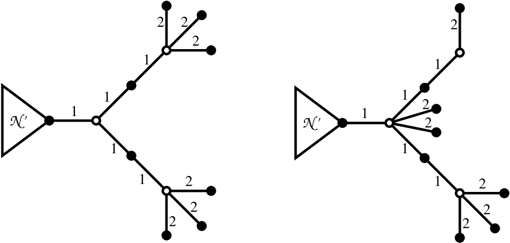
What remains is to study more attentively the structure of the non-repeating branch $\cal N$ . Here we consider the following cases:

•

The height of $\cal N$ is 1, that is, ${\cal N^{\prime}}=\varnothing$ .
•

The height of $\cal N$ is 2.
•

The height of $\cal N$ is 3 or more, and $\cal N$ starts with a path having the weights $1$ , $s$ , $1$ where $s$ is equal to 1 or 2.
•

The height of $\cal N$ is 3 or more, and $\cal N$ starts with a path having the weights $1$ , $s$ , $s+1$ where $s$ is equal to 1 or 2.

The height of $\cal N$ equal to 1 case is trivial: we get the tree $L$ (Figure 19).

The height of $\cal N$ equal to 2 case is illustrated in Figure 42. If the weight of the leaves of the non-repeating branch is equal to 2 then, whatever is their number, the reattachment shown on the left changes the tree since the new tree has one leaf less than the initial one. If the weight of the leaves of the non-repeating branch is equal to 1 then the reattachment shown on the right also changes the tree unless there is only one leaf in the non-repeating branch. The latter case gives us the tree $M$ (Figure 19).

Assume now that the height of the non-repeating branch is $\geq 3$ , and this branch contains a path with the weights 1, $s$ , 1, see the upper tree in Figure 43. First of all, we remark that the subtree $\cal A$ may be interchanged with a chain of length 2 attached to the vertex $p$ . Then, according to the principle “all branches except maybe one are isomorphic”, two situations may occur. First, we could thus create two repeating branches $\cal U$ attached to the vertex $q$ , see the tree in the middle. But such a tree would contain repeating branches of the type $(1,s,1)$ which contradicts our supposition. The other possibility is that $\cal A$ is equal to the chain which was attached to $p$ . Then we get a vertex $r$ (see the lower tree) which is of degree 2 and is incident to two edges of weights 1 and 1. Therefore, according to Proposition 5.18, the edge of weight $s$ , which is not a leaf, cannot have weight 2; hence, $s=1$ . Finally, we affirm that ${\cal C}=\varnothing$ , otherwise it could be reattached to the vertex $p$ and we would get three different trees attached to $q$ . The resulting tree is shown in Figure 43, bottom. If ${\cal B}=\varnothing$ we get the tree $S$ (Figure 20). If ${\cal B}\neq\varnothing$ then, again according to the principle “all branches except maybe one are isomorphic”, $\cal B$ must be equal to a chain of weights 1, 1, 2, and we get the tree $R$ (Figure 20), since otherwise a tree would contain repeating branches of the type $(1,s,1)$ . (Note that in the last case we obtain the tree $T$ which is considered in Proposition 5.25 which treats the case of repeating branches of the type $(1,t,1)$ .)

Finally, consider the case when the non-repeating branch is of height $\geq 3$ and contains a path with the weights 1, $s$ , $s+1$ , see Figure 44. We affirm that in this case $s=1$ and all the three subtrees $\cal A$ , $\cal B$ , $\cal C$ are empty, so that we get the tree $N$ of Figure 19 (and what we call “non-repeating branch” is in this case equal to the repeating branches). Indeed, the tree contains a path with the weights 1, 1, 1; therefore, according to Proposition 5.14, the only possible weights are 1 and 2, so $s=1$ . Now, if ${\cal A}\neq\varnothing$ then it could be reattached to the vertex $q$ thus producing a tree with one more leaf. Therefore, ${\cal A}=\varnothing$ . Then, $\cal C$ is also empty since $\cal A$ and $\cal C$ can be interchanged. Finally, if ${\cal B}\neq\varnothing$ then there are two possibilities. Either $\cal B$ is a bunch of leaves of weight 2; but then it can be reattached to the vertex $p$ . Or $\cal B$ is a number of copies of the long branch growing out of the vertex $r$ ; but then, once again, we would create repeating branches of the type $(1,t,1)$ .

Proposition 5.24 is proved. $\Box$

5.6 Trees with repeating branches of the type $(1,t,1)$

In this subsection we classify unitrees which have crossroads of the type $(1,t,1)$ .

Proposition 5.25 (Branches of type $(1,t,1)$ )

A unitree which has at least one crossroad of type $(1,t,1)$ belongs to one of the types $I$ , $Q$ , or $T$ .

Proof.

First of all, observe that by Lemma 5.10 the subtree $\cal B$ is a collection of copies of the subtree $\cal U$ , and the subtree $\cal A$ is a collection of copies of the subtree $\cal V$ (see Figure 45). Further, an $sts$ -operation, applied to the first tree of Figure 45 gives the second tree shown in this figure. This image implies that there are only two repeating branches growing from the vertex $p$ , otherwise the tree would certainly change. Now, looking at the vertex $q$ of the second tree of Figure 45 we see that either ${\cal N}={\cal U}$ or ${\cal N}={\cal W}$ . If ${\cal N}={\cal W}$ then the initial tree would look like the third tree of the same figure. Then we could once again apply an $sts$ -transformation and make the long branch even longer, and one of the repeating branches, shorter (see the fourth tree of the figure), which would give us three different branches attached to $p$ . Hence, ${\cal N}={\cal U}$ . In particular, we have proved that whenever a unitree has a crossroads of type $(1,t,1)$ the corresponding non-repeating branch is a subtree of the repeating branch.

Now, it follows from ${\cal N}={\cal U}$ that the first tree of Figure 45 has a (unique) center at the vertex $p$ while the second one has a (unique) center at the vertex $r$ . Hence, the vertex $p$ of the first tree must correspond to the vertex $r$ of the second one, and thus we must have $t=1$ and ${\cal B}={\cal N}={\cal U}$ . Therefore, the tree has the form shown in Figure 46, with the same number $l\geq 1$ of branches growing out of the vertices $u$ and $v$ .

If ${\cal C}=\varnothing$ then we get a tree of the type $I$ . Thus we may assume that ${\cal C}$ is non-empty. Observe first that $l=1$ . Indeed, if $l>1$ then $\cal V$ is a repeating branch. Furthermore, since ${\cal C}$ is non-empty, $\cal V$ is either $(1,t,t+1)$ -branch or $(1,t,1)$ -branch. The first case is impossible by Lemma 5.23, while the second case is impossible since, as we have shown in the previous paragraph, here the corresponding non-repeating branch should be a subtree of $\cal V$ , and this is not so.

If $\cal C$ is a collection of leaves, then the transformation of Figure 32 shows that all leaves are of weight 1. Moreover, $\cal C$ contains not more than one leaf since otherwise we could transfer all the other leaves to the vertex $v$ , which would change the tree. Therefore, in this case we get the tree $Q$ . Finally, if $\cal C$ is not a collection of leaves, then $\cal W$ is a repeating branch of height at least 3, which, as above, is necessarily of type $(1,t,t+1)$ , and Lemma 5.23 implies that $\cal W$ has the form shown in Figure 37 on the left, where the number of leaves is equal to one since otherwise we could transport all the leaves but one to the vertex $w$ . Therefore, in this case we get the tree $T$ .

Proposition 5.25 is proved. $\Box$

5.7 Proof of the uniqueness of unitrees

Our main tool will be “cutting and gluing leaves”, though these operations will be carried out not with the trees themselves but with their passports; the trees must be kept in mind for an intuitive understanding of the proof. We do not repeat every time that “the same reasoning remains valid if we interchange black and white”.

(A) There is only one black vertex (see Figure 11); therefore, all white vertices must be adjacent to it, which means that they are leaves. The uniqueness is evident.

The uniqueness proofs for the cases from (B) to (E) all follow the same lines. If the structure of a passport implies the existence of a leaf of degree, say, $s$ , then the only way to construct a corresponding tree is to glue an edge of the weight $s$ to a vertex of the opposite color of a tree having one less edge. Furthermore, in the initial (bigger) tree this edge can only be attached to a vertex of degree bigger than $s$ . If the smaller tree is a unitree (and usually it is by induction), and if there is essentially one way to attach the new edge to it, then the bigger tree is also a unitree. In certain cases more than one way of attaching a new edge may exist, but they all lead to isomorphic trees.

(B) Let us consider, for example, the case of an odd length, and examine not the tree itself but its passport $(\alpha,\beta)$ . For this tree, $\alpha$ and $\beta$ are the same: $\alpha=\beta=((s+t)^{k},s)$ . The passport implies that there are two vertices of degree $s$ , a black one and a white one, while all the other vertices, both black and white, are of degree $s+t$ . These latter vertices cannot be leaves since otherwise there should exist vertices of a bigger degree to which such leaves would be attached. A tree must have at least two leaves. We conclude that there are exactly two leaves, and they are vertices of degree $s$ . They are connected to the tree by edges of the weight $s$ . The degree of the vertex to which such a leaf is attached is $s+t$ , and its color is opposite to the color of the leaf.

Now let us cut off one of these leaves, for example, the white one. Then we get a tree with one less edge and with the passport $\alpha=((s+t)^{k-1},s,t)$ and $\beta=(s+t)^{k}$ . This passport corresponds to the chain tree of smaller (and even) length. We may inductively suppose that this tree is a unitree. The vertex of degree $t$ of this tree is a leaf. Now, we must make an operation which would simultaneously fulfill the following three goals:

•

it re-attaches back a white leaf of weight $s$ to the smaller tree;
•

it makes the black vertex of degree $t$ in the smaller tree to disappear;
•

it makes to appear an additional, $k$ th black vertex of degree $s+t$ , to the already existing $k-1$ ones.

It is clear that the only way to do all that is to attach this white leaf of weight $s$ to the black vertex of degree $t$ . This operation re-creates the initial chain-tree.

The proof for an even length repeats the previous one almost word to word, only the leaves are now of the same color and of degrees $s$ and $t$ . The base of induction is a tree consisting of a single edge, which is obviously unique.

(C) The passport of a tree of the type $C$ is $\alpha=(ks+t,s^{l})$ , $\beta=(ls+t,s^{k})$ . We affirm that there exists a leaf of degree $s$ . Indeed, a tree must have at least two leaves, and the vertex of the biggest degree cannot be a leaf. The biggest degree is either $ks+t$ , or $ls+t$ , or both.

Suppose that we have a black leaf of degree $s$ . Then it has to be attached to the only white vertex of degree bigger than $s$ , which is the white vertex of degree $ls+t$ . Cut this leaf off. We get a smaller tree, with one less edge, with $l$ being replaced with $l-1$ . This tree is a smaller instance of $C$ which may supposed to be a unitree by induction. (Note that in particular cases it can also be of type $B$ , or even of $A$ , the latter one when $l$ was equal to 1.)

Now we no longer work with the passports but with the trees. We know the smaller tree since it is unique, and we must re-attach the previously cut-off black leaf to a white vertex of this smaller tree. Here two cases may take place.

1.

If $s\neq t$ , or even if $s=t=1$ but $l\neq 1$ , the initial (bigger) tree did not have a white vertex of degree $2s$ . Therefore, we cannot attach the cut-off leaf to a white vertex of degree $s$ . Hence, the only vertex to which it can be attached is the white vertex of degree $(l-1)s+t$ .
2.

If $s=t=1$ and $l=1$ then the smaller tree is the star with all its leaves being of degree 1. Then we may re-attach the leaf to any one of them, the resulting tree will be the same.

There is an additional subtlety here. The planar structure of our trees means that we must choose not only a vertex to which we attach a new edge. We must also choose an angle between neighboring edges incident to the vertex of attachment, and to insert the leaf into the angle between these edges. If there are $m$ edges incident to a vertex, there also are $m$ angles between them, and therefore $m$ ways of placing the new edge. But, obviously, in our case all these ways give the same plane tree, see Figure 13.

(D) Two black vertices of degree $2s+t$ cannot be leaves. Therefore, there exists a leaf of degree $s$ or $s+t$ . Cut it off, and we get either $C$ or $E_{1}$ . Indeed, if the cut-off (white) leaf was of degree $s$ , and was attached to one of the black vertices of degree $2s+t$ (there are no other black vertices), then the passport of the smaller tree becomes $\alpha=(2s+t,s+t)$ , $\beta=((s+t)^{2},s)$ . This passport corresponds to the pattern $E_{1}$ , with $l=1$ and the length of the chain equal to 4. The uniqueness of the corresponding tree will be proved in a moment. The only way to glue a leaf of degree $s$ to this tree and to create a vertex of degree $2s+t$ instead of vertex of degree $s+t$ is to glue this leaf to the vertex of degree $s+t$ .

If, on the other hand, the cut-off (white) leaf was of degree $s+t$ , and was attached to one of the black vertices of degree $2s+t$ , then the passport of the smaller tree becomes $\alpha=(2s+t,s)$ , $\beta=(s+t,s^{2})$ . This passport corresponds to a tree of type $C$ , with $k=2$ and $l=1$ . The uniqueness of such a tree was proved above. Then the only way to glue back the leaf of degree $s+t$ is to glue it to the black vertex of degree $s$ of the smaller tree.

It is easy to see that in both cases we get the same tree $D$ .

(E) The proof is similar to the cases considered above, so we will shorten our presentation. Consider first the cases $E_{3}$ and $E_{4}$ . All the vertices except two are of degree $s+t$ ; the two remaining ones are of degrees $(k+1)s+kt$ and $(l+1)s+lt$ for $E_{3}$ , and $(k+1)s+kt$ and $ls+(l+1)t$ for $E_{4}$ . Without loss of generality we may suppose that $(k+1)s+kt$ is the bigger of the two; therefore, it cannot be a leaf. For $E_{4}$ , the “second best” vertex cannot be a leaf either since it has the same color. For $E_{3}$ , if $k>l$ , the vertex of degree $(l+1)s+lt$ might in principle be a leaf. Whatever is the case, there exists a leaf of degree $s+t$ . Cut it off, and we obtain a smaller tree, with the possible pattern transitions as follows: $E_{4}\to E_{4}$ ; $E_{3}\to E_{3}$ ; $E_{4}\to E_{2}$ ; or $E_{3}\to E_{1}$ , the latter two maybe with renaming the variables.

Now, for the cases $E_{1}$ and $E_{2}$ the situation is similar. All the vertices except two are of degree $s+t$ . The vertex of the biggest degree cannot be a leaf. Therefore, there exists a leaf of degree $s$ or $s+t$ . Cut it off, and we get a smaller tree, with the possible pattern transitions as follows: $E_{1}\to E_{1}$ ; $E_{1}\to E_{2}$ ; $E_{2}\to E_{1}$ ; $E_{2}\to E_{2}$ , or we may arrive to the patterns $A$ or $B$ .

What remains now is to see that there is only one way to re-attach the cut-off leaf to the smaller unitree.

(F, H, I, Q) The trees $F$ , $H$ , $I$ , $Q$ are ordinary; therefore, the enumerative formula (13) can be applied.

If $m\neq l$ , a tree of the series $F$ is asymmetric, and therefore its contribution to (13) is 1. Now, formula (13) in this case gives 1; therefore, there is no other tree with this passport.

When $m=l$ , a tree of the series $F$ is symmetric, with the rotational symmetry of order $k$ . Therefore, its contribution to (13) is $1/k$ . Now, the formula itself gives $1/k$ ; therefore, there is no other tree in this case either.

For the trees of the series $H$ , formula (13) gives 1 when $k\neq l$ , and gives $1/2$ when $k=l$ . This corresponds to the symmetry order of these trees: they are asymmetric when $k\neq l$ , and symmetric of order 2 when $k=l$ .

The trees of the series $I$ are asymmetric, and formula (13) gives 1.

The tree $Q$ is asymmetric, and formula (13) gives 1.

(G) The tree has $km$ vertices and hence $km-1$ edges. Since the total weight is $km$ , there exists exactly one edge of weight 2 while all the other edges are of weight 1. The only white vertex to which the edge of weight 2 can be attached is the vertex of degree $k$ , since all the other white vertices are of degree 1. The rest is obvious.

(J) All white vertices are of degree 2; therefore, a weight of an edge can only be 1 or 2. There are only three black vertices, their degrees being 4, $2k+1$ , $2k+1$ . Therefore, the black vertices cannot be leaves since such leaves could not be attached to a white vertex of degree 2; thus, all the leaves are white. A white vertex which is not a leaf must have two black neighbors; therefore, there are exactly two white vertices which are not leaves: they are “intermediate” white vertices between the black ones. The edges incident to them are both of weight 1. The black vertex of degree 4 cannot have two incident edges of weight 2 since these edges should be leaves, and such a tree would not be connected; it cannot have four incident edges of weight 1 either since such a tree should need more than three black vertices. Therefore, the weights of the edges attached to this vertex must be 2, 1, 1, and the edge of weight 2 is a leaf. The rest is obvious.

(P) All black vertices are of degree 5, all white ones are of degree 3. Therefore, black vertices cannot be leaves. Arguing now as in the case (J) we conclude that there are exactly three white leaves, implying easily that there exists only one tree with this passport.

(K, L, M, N, O, R, S, T) The proof of all these cases follows the same pattern.

Let us take, for example, the tree $O$ . Its passport is $(5^{4},2^{10})$ . Therefore, the number of vertices is $4+10=14$ and the number of edges is 13, while the total weight is $5\cdot 4=2\cdot 10=20$ . Thus, the overweight is 7, and it must be distributed among the edges.

Now, no edge can have a weight greater than 2 since the degrees of white vertices are all equal to 2. Therefore, the tree $O$ has seven edges of weight 2. Moreover, all of them are leaves; indeed, if something were attached to the white end of such an edge then this white end would have a degree greater than 2.

The same reasoning may be carried out for all the above cases, with their respective overweights and numbers of leaves of weight 2.

Now, let us cut off all the leaves of weight 2. What remains is an ordinary tree, and we must verify that it is a unitree. Usually it is immediately obvious since the ordinary tree in question is very small; otherwise, we may apply formula (13), or else we may remark that such a tree belongs to one of the previously established cases. For example, for the tree $T$ what remains after cutting off the leaves of weight 2 is the tree $Q$ .

The last step consists in proving that there is only one way to glue back to this ordinary unitree the leaves of weight 2 that were previously cut off. For example, in the case $O$ the ordinary unitree has black vertices of degrees 3, 1, 1, 1, and we have, by gluing to them seven edges of weight 2, made these degrees equal to 5, 5, 5, 5. Obviously, there is only one way to do that. In fact, in certain cases there are several ways of gluing but they give the same result because of a symmetry of the underlying ordinary tree. For the tree $L$ , there is an additional condition we must satisfy: white leaves can only be attached to black vertices.

Theorem 5.4 is proved. $\Box$

6 Other combinatorial Galois invariants

The theory of dessins d’enfants studies combinatorial invariants of the Galois action on dessins. These invariants have various levels of generality. The most general (and the most simple) one is the passport; the subject of this paper is precisely the case when the passport alone guarantees the definability of a dessin over ${\mathbb{Q}}$ . But our exposition would be incomplete if we did not mention several other Galois invariants which lead to further examples of dessins and DZ-triples defined over ${\mathbb{Q}}$ .

6.1 Composition

The following proposition is obvious.

Proposition 6.1 (Composition)

Let $f=f(x)$ and $h=h(t)$ be two rational functions such that:

•

$f$ is a Belyi function, with the corresponding dessin $D_{f}$ ;
•

$h$ is a function $($ not necessarily a Belyi one $)$ , all of whose critical values are either vertices or face centers of $D_{f}$ .

Then the function $F(t)$ obtained as a composition

F(t)=f(h(t)),\qquad\mbox{\rm that is},\qquad F\,:\,\overline{{\mathbb{C}}}\,\stackrel{{\scriptstyle h}}{{\longrightarrow}}\,\overline{{\mathbb{C}}}\,\stackrel{{\scriptstyle f}}{{\longrightarrow}}\,\overline{{\mathbb{C}}},

is a Belyi function. If, furthermore, both $f$ and $h$ are defined over ${\mathbb{Q}}$ , then, obviously, the same is true for $F$ .

The above proposition gives us a very general method of constructing Belyi functions with all its finite poles being simple, or, in other words, Belyi functions corresponding to weighted trees.

Corollary 6.2 (Decomposable weighted trees)

Suppose that the functions $f$ and $h$ of the above proposition satisfy the following properties:

•

the dessin $D_{f}$ corresponds to a weighted tree, that is, all its finite faces are of degree $1$ ;
•

$h$ is a polynomial all of whose critical values except infinity are vertices of $D_{f}$ .

Then all the finite faces of the dessin $D_{F}$ corresponding to the Belyi function $F(t)=f(h(t))$ are of degree $1$ . If, furthermore, both $f$ and $h$ are defined over ${\mathbb{Q}}$ , then, obviously, the same is true for $F$ .

Proof.

Since $h$ is a polynomial, the only poles of $F=f\circ h$ , except infinity, are the preimages of the simple poles of $f$ , i. e., the preimages of the centers of the small faces of $D_{f}$ . Since $h$ is not ramified over these simple poles, they remain simple for $F$ , and each of them is “repeated” $\deg h$ times. $\Box$

Example 6.3 (Composition 1)

Consider the following functions:

f\,=\,-\,\frac{64\,x^{3}(x-1)}{8\,x+1}\,,\qquad u\,=\,\frac{1}{5^{5}}\cdot(t^{2}+4)^{3}(3\,t+8)^{2}\,.

Here $f$ is a Belyi function corresponding to the upper left dessin in Figure 47, and $u$ is a Belyi function corresponding to the lower left dessin.

Substituting $x=u(t)$ in $f$ we obtain a Belyi function $F$ corresponding to the dessin shown on the right of Figure 47. It is obvious that the combinatorial orbit of the dessin $D_{F}$ consists of more than one element: for example, the petals attached to the vertices of degrees 9 and 6 can be cyclically arranged in many different ways. Still, $F\in{\mathbb{Q}}(x)$ by construction.

Note that the dessins $D_{f}$ and $D_{u}$ serving as building blocks for the above example both belong to the classification we have established in Section 5: they both correspond to unitrees, and it is their passports that guarantee that they are defined over ${\mathbb{Q}}$ . We don’t have a simple way of constructing more general examples over ${\mathbb{Q}}$ (when, e. g., the polynomial $u$ has more than two critical values with prescribed positions at vertices of $D_{f}$ ).

Example 6.4 (Composition 2)

Another example, based on the same function $f$ , is as follows. We have

f-1\,=\,-\,\frac{(8\,x^{2}-4\,x-1)^{2}}{8\,x+1}\,,

so the white vertices of the dessin $D_{f}$ (which are not shown explicitly in Figure 47) are the roots of $8\,x^{2}-4\,x-1$ , that is, they are equal to $(1\pm\sqrt{3})/4$ . Now, the critical values of the polynomial

v\,=\,\frac{1}{3}\,t^{3}-\frac{3}{4}\,t+\frac{1}{4}\,,

that is, the values of $v$ at the roots of $v^{\prime}=t^{2}-3/4$ , are equal to exactly $(1\pm\sqrt{3})/4$ . Therefore, the composition $G(t)=f(v(t))$ is once again a Belyi function, and all its poles except infinity are simple. The corresponding dessin is shown in Figure 48.

It is obvious that the dessin $D_{G}$ is not the only one having the passport $(3^{3}1^{3},4^{2}2^{2})$ . For example, the two “vertical” edges can both be put above, or both can be put below the horizontal axis, or they can be cut off and attached to the leftmost white vertex of degree 2 (the one on the loop), or to the rightmost one (the one on the horizontal segment). Nevertheless, the dessin thus obtained is defined over ${\mathbb{Q}}$ by construction.

Now the dessins $D_{F}$ and $D_{G}$ , being defined over ${\mathbb{Q}}$ , may themselves serve for a similar construction: if, for example, $w$ is a polynomial with coefficients in ${\mathbb{Q}}$ whose critical values are vertices of $D_{G}$ , then the function $H=G\circ w=f\circ v\circ w$ is a Belyi function corresponding to a dessin $D_{H}$ , all of whose finite faces are small. In such a composition, only $f$ has to be a Belyi function while the subsequent terms may have more than three critical values.

Remark 6.5 (Symmetric trees)

The group of the orientation preserving automorphisms of a plane tree is always cyclic. If it is ${\mathbb{Z}}_{k}$ then the Belyi function for the corresponding map is $F(x)=f(x^{k})$ where $f$ is the Belyi function for the map corresponding to a single branch of the tree (the vertex of this branch, which will become the center of the symmetric tree, must be put to the origin). Among the unitrees classified in Section 5, the trees $N$ and and $R$ are symmetric (of order 3 and 2 respectively). Some elements of the infinite series may also be symmetric (for special values of parameters).

We leave it to the reader to see that the series $H$ and $I$ are compositions (although the composition in this case is not reduced to a rotational symmetry), and that a multiplication of all the weights of the edges of a tree by a factor $d$ can be represented as a composition with the following Belyi function:

f(x)\,=\,\frac{x^{d}}{x^{d}-(x-1)^{d}}\,,\qquad\mbox{hence}\qquad f(x)-1\,=\,\frac{(x-1)^{d}}{x^{d}-(x-1)^{d}}\,.

6.2 Primitive monodromy groups

Definition 6.6 (Primitive and special groups)

A permutation group of degree $n$ acting on a set $X$ , $|X|=n$ , is called imprimitive if the set $X$ can be subdivided into $m$ disjoint blocks $X_{1},\ldots,X_{m}$ of equal size $|X_{i}|=n/m$ , where $1<m<n$ , such that an image of a block under the action of any element of the group is once again a block. A permutation group which is not imprimitive is called primitive. A primitive permutation group not equal to ${\rm S}_{n}$ or ${\rm A}_{n}$ is called special.

It is known (see [17]) that a covering is a composition of two or more coverings of smaller degrees if and only if its monodromy group is imprimitive. Thus, a covering which is not a composition has a primitive monodromy group. However, in a vast majority of cases this group is equal to either ${\rm S}_{n}$ or ${\rm A}_{n}$ , for a very simple reason: a permutation group generated by a randomly chosen pair of permutations is ${\rm S}_{n}$ or ${\rm A}_{n}$ with a probability close to 1. This is why special groups are of a particular interest: since the monodromy group is a Galois invariant, such a group gives an additional invariant in the absence of the composition.

In the case of weighted trees, that is, in the case of coverings realized by Belyi functions with all poles except one being simple, the monodromy group must contain a permutation of the cycle structure $(n-r,1^{r})$ : it is the monodromy permutation corresponding to a loop around infinity on the Riemann sphere. Motivated by our study of weighted trees, Gareth A. Jones classified all special permutation groups containing such a permutation, see [15] (2012). In particular, it is shown that in all such cases $r\leq 2$ . This property is based on two results. The first is an old theorem by Jordan (1871) [16] stating that a primitive group containing a permutation with the cycle structure $(n-r,1^{r})$ is $(r+1)$ -transitive. The second is the complete list of multiply transitive groups: it is based on the classification theorem of finite simple groups.

The classification due to Jones looks as follows (we use standard notation for projective, cyclic and affine groups and for the Mathieu groups):

Theorem 6.7 (G. Jones’s classification)

Let $G$ be a primitive permutation group of degree $n$ not equal to ${\rm S}_{n}$ or ${\rm A}_{n}$ . Suppose that $G$ contains a permutation with cycle structure $(n-r,1^{r})$ . Then $r\leq 2$ , and one of the following holds:

1.
$r=0$ and either
- (a)
  
  ${\rm C}_{p}\leq G\leq{\rm AGL}_{1}(p)$ with $n=p$ prime, or
- (b)
  
  ${\rm PGL}_{d}(q)\leq G\leq{\rm P{\Gamma}L}_{d}(q)$ with $n=(q^{d}-1)/(q-1)$ and $d\geq 2$ for some prime power $q=p^{e}$ , or
- (c)
  
  $G={\rm L}_{2}(11)$ , ${\rm M}_{11}$ or ${\rm M}_{23}$ with $n=11$ , $11$ or $23$ respectively.
2.
$r=1$ and either
- (a)
  
  ${\rm AGL}_{d}(q)\leq G\leq{\rm A{\Gamma}L}_{d}(q)$ with $n=q^{d}$ and $d\geq 1$ for some prime power $q=p^{e}$ , or
- (b)
  
  $G={\rm L}_{2}(p)$ or ${\rm PGL}_{2}(p)$ with $n=p+1$ for some prime $p\geq 5$ , or
- (c)
  
  $G={\rm M}_{11}$ , ${\rm M}_{12}$ or ${\rm M}_{24}$ with $n=12$ , $12$ or $24$ respectively.
3.

$r=2$ and ${\rm PGL}_{2}(q)\leq G\leq{\rm P{\Gamma}L}_{2}(q)$ with $n=q+1$ for some prime power $q=p^{e}$ .

Example 6.8 (A tree with a special monodromy group)

There are six weighted trees of degree $n=8$ with the passport $(7^{1}1^{1},2^{3}1^{2},6^{1}1^{2})$ . One may expect that their common moduli field would be an extension of ${\mathbb{Q}}$ of degree 6. However, this is not the case. Five trees out of six have the monodromy group ${\rm S}_{8}$ , while the remaining one, shown in Figure 49 (left) has the monodromy group ${\rm PGL}_{2}(7)$ . Therefore, this tree is defined over ${\mathbb{Q}}$ . The other trees form a single Galois orbit over a field of degree 5.

In order to establish that the group in question is indeed ${\rm PGL}_{2}(7)$ we may proceed as follows. First, we draw the bicolored map represented by this tree, as it is done in Figure 49, right. Then, we label the edges of the map and write down two permutations: the first one represents the cyclic order of the edges around its black vertices in the counterclockwise direction, while the second one represents the cyclic order of the edges around their white vertices in the same direction. In our case these permutations are

a\,=\,(1,7,6,5,4,8,3),\qquad b\,=\,(1,2)(3,8)(6,7).

The permutation corresponding to the faces is

c\,=\,(ab)^{-1}\,=\,(1,2,3,4,5,6),

so that $abc=1$ . The cycle $c$ can be read in the picture by going around the outer face. Note that the cycle structures of $a$ , $b$ and $c$ are $7^{1}1^{1}$ , $2^{3}1^{2}$ and $6^{1}1^{2}$ , respectively. Then, the monodromy group is

G\,=\,\langle a,b\rangle\,=\,\langle a,b,c\rangle.

Using Maple it is easy to find out that $|G|=336$ , and the only transitive subgroup of ${\rm S}_{8}$ of order 336 is ${\rm PGL}_{2}(7)$ (see, for example, [5]). For the other five trees with the same passport the same Maple package shows that the size of their monodromy group is $40\,320=8!$ , so the group in question is ${\rm S}_{8}$ .

Example 6.9 ( ${\rm PGL}_{2}(7)$ once again)

One more example is shown in Figure 50. There are five trees with the passport $(6^{1}1^{2},3^{2}1^{2},6^{1}1^{2})$ . One of them is symmetric and therefore forms a Galois orbit containing a single element and thus defined over ${\mathbb{Q}}$ . Three trees have the monodromy group ${\rm S}_{8}$ ; they form a cubic Galois orbit. Finally, the remaining tree shown in Figure 50 has the monodromy group ${\rm PGL}_{2}(7)$ . Therefore, it forms a Galois orbit in itself and is thus defined over ${\mathbb{Q}}$ .

6.3 Duality and self-duality

A dual to a map is usually constructed as follows. First, one puts a new vertex inside every face of the initial map: this vertex is called “center” of the face. Then, the centers of the adjacent faces are connected by edges in such a way that every edge of the initial map is crossed in its “middle point” by a new edge. A dual of a dual is the initial map.

For the bicolored maps a specific variant of the above construction is used, when only black vertices are considered as vertices, while the white vertices play the role of the edge midpoints. An association is thus made between the faces of the initial map and black vertices of the dual map. The white vertices belong to both maps. More exactly, a center of a face is connected by edges with all the white verices lying on the border of the face: see an example in Figure 51 where the initial map is shown in an unbroken line, and its dual, in a dashed line; the black vertices of the dual map are designated by the little squares.

From the point of view of Belyi functions, if $f(x)$ is a Belyi function for the initial map then $1/f(x)$ is a Belyi function for its dual. Indeed, $1/y$ interchanges 0 and $\infty$ while leaving 1 untouched. Therefore, the former poles become roots (i. e., black vertices), and vice versa.

Definition 6.10 (Self-dual map)

A bicolored map is called self-dual if it is isomorphic to its dual map.

Of course, the fact that a map is self-dual does not mean that $f=1/f$ where $f$ is its Belyi function. It means that $1/f(x)=f(w(x))$ where $w(x)$ a linear fractional transformation of the variable $x$ . The self-duality is an invariant of the Galois action: if a function satisfies an algebraic relation while the other function does not satisfy the same relation, they cannot belong to the same Galois orbit.

A weighted tree represents a map whose all faces except one are of degree 1. Therefore, its dual map must have all its black vertices except one being of degree 1. This can only happen if the dual map corresponds to a weighted tree of diameter 4: it has a black vertex of a degree greater than 1 (its central vertex), while all its black leaves are of degree 1. Therefore, if we are interested in self-dual maps which correspond to weighted trees then we must consider only the trees of diameter 4. The condition on the branches of such trees in order for them to be dual to each other is shown in Figure 52.

Now we are ready to give an example where the self-duality plays the role of a Galois invariant.

Example 6.11 (Self-duality as a Galois invariant)

Let us take two integers $p$ and $q$ , $p<q$ , and consider the following passport of degree $n=2p+2q-2$ :

•

there is a black vertex of degree $p+q$ (the center), and $p+q-2$ black vertices of degree 1 (the leaves);
•

there are two white vertices, of degrees $2p-1$ and $2q-1$ respectively;
•

the above data imply that the trees have $p+q$ edges, and therefore the outer face is of degree $p+q$ , the same as the degree of the central black vertex.

There are exactly $2p-1$ trees with this passport. Their general appearance is shown in Figure 53. Here the parameters take the following values: $s=1,2,\ldots,2p-1$ while

t=(p+q)-s,\quad k=(2p-1)-s,\quad l=(2q-1)-t.

Among all these trees, only one is self-dual: it corresponds to the values $s=p$ , $t=q$ , $k=p-1$ , and $l=q-1$ . Therefore, this tree is defined over ${\mathbb{Q}}$ .

(In this example both branches are dual to themselves. An attempt to make one branch dual to the other leads to the equality $p=q$ , but we have supposed that $p<q$ .)

Remark 6.12 (Example 6.9 revisited)

All the five trees with the passport $(6^{1}1^{2},3^{2}1^{2},6^{1}1^{2})$ considered in Example 6.9 are self-dual. Therefore, for them the self-duality cannot serve as an additional Galois invariant leading to a splitting of the combinatorial orbit into two (or more) Galois orbits.

6.4 A sporadic example

The world of dessins d’enfants is rich with various specific cases. Let us consider, for example, the set of dessins shown in Figure 54. They constitute a combinatorial orbit for the passport $(\alpha,\beta,\gamma)$ where $\alpha=3^{10}$ , $\beta=2^{15}$ , and $\gamma=24^{1}1^{6}$ . We might naïvely suppose that this combinatorial orbit also constitutes a Galois orbit; if this were the case, this orbit would be defined over a field of degree 4 (since it has four elements). However, the reality is more complicated and, in fact, more exciting.

Namely: the dessin $a$ is the only one having a rotational symmetry of order 3 around a black vertex. Therefore, the singleton $\{a\}$ constitutes a Galois orbit. Two dessins $b$ and $c$ are the only ones which have rotational symmetry of order 2, the center being a white vertex (we recall that the white vertices, being all of degree 2, are not shown explicitly in the picture). Therefore, the set $\{b,c\}$ must also be taken apart from the combinatorial orbit. There are two a priori possibilities: $b$ and $c$ may make two Galois orbits, both defined over ${\mathbb{Q}}$ , or they may make a single Galois orbit defined over a quadratic field. But any map whose Belyi function is defined over a real field must be axially symmetric since it remains invariant under the complex conjugation. This observation excludes the possibility of two orbits over ${\mathbb{Q}}$ , and it also excludes a real quadratic field. We may conclude that the set $\{b,c\}$ constitutes a single Galois orbit defined over an imaginary quadratic field.

The dessin $d$ is not symmetric and does not have any other specific combinatorial features. But it remains solitary, and therefore it constitutes a Galois orbit all by itself. Since the orbits $\{a\}$ and $\{d\}$ consist of a single element, their Belyi functions are defined over ${\mathbb{Q}}$ . Thus, the dessin $d$ is defined over ${\mathbb{Q}}$ for no other reason than the fact that it remains alone after all the other Galois orbits are taken away.

This combinatorial orbit is markworthy for the reason that different authors returned to it, or to some of its elements, many times. The Belyi function for $a$ was computed by Birch and already appeared in [4] (1965); the one for $d$ was computed 35 years later by Elkies [10] (2000). All the four Belyi functions were independently computed by Shioda [23] (2004). In particular, he found out that the orbit $\{a,b\}$ is defined over the field ${\mathbb{Q}}(\sqrt{-3})$ . Shioda had already used as a starting point the above combinatorial orbit; the other authors have apparently made a “blind” search.

Our combinatorial approach does not make the computational part of the work any easier. Its advantage is elsewhere. It consists in the fact that, before any computation, we may be sure of the following.

•

There exist exactly four non-equivalent Belyi functions with the passport $(3^{10},2^{15},24^{1}1^{6})$ ; here “non-equivalent” means that they cannot be obtained from one another by a linear fractional change of variables.
•

Belyi functions corresponding to $a$ and $d$ are defined over ${\mathbb{Q}}$ .
•

Belyi function corresponding to $a$ is a rational function in $x^{3}$ (because of the threefold symmetry of the dessin $a$ ).
•

Belyi functions for the orbit $\{b,c\}$ are defined over an imaginary quadratic field.

More examples similar to this one are given below.

6.5 Sporadic examples of Beukers and Stewart [3]

All the examples in this section are borrowed from the paper [3] by Beukers and Stewart, which was one of the sources of inspiration for our study. In their paper, the authors consider only the case of powers of polynomials. Namely, they look for polynomials $A$ and $B$ , defined over ${\mathbb{Q}}$ , for which the degree $\deg\,(A^{p}-B^{q})$ attains its minimum. The degrees of polynomials in question are $\deg A=qr$ , $\deg B=pr$ where the parameter $r$ may be greater than 1. The passport of the corresponding tree is $(p^{qr},q^{pr})$ .

The authors find, as we do, several infinite series of DZ-triples (which they call Davenport pairs), and several sporadic examples. The first such example, for which $(p,q,r)=(5,2,2)$ , corresponds to our sporadic tree $O$ . The next one, $(p,q,r)=(5,3,1)$ , corresponds to the sporadic tree $P$ . However, the subsequent examples do not correspond to anything we have found up to now. What is going on?

It turns out that here we encounter once again the phenomenon that we already explained in Section 6.4.

Example 6.13 ( $(p,q,r)=(7,3,1)$ )

There exist two trees corresponding to the passport $(7^{3},3^{7})$ : they are shown in Figure 55. We see that one of the trees is symmetric, with the symmetry of order 3, while the other one is not. Therefore, this combinatorial orbit splits into two Galois orbits, and hence both trees are defined over ${\mathbb{Q}}$ . The left-hand one corresponds to the example given in [3].

Note that an axial symmetry is not a Galois invariant.

Example 6.14 ( $(p,q,r)=(8,3,1)$ and $(10,3,1)$ )

The situation for the passports $(8^{3},3^{8})$ and $(10^{3},3^{10})$ is similar to the previous one. For the first passport there are two trees, and one of them is symmetric while the other is not (see Figure 56); therefore, both are defined over ${\mathbb{Q}}$ . For the second passport there are three trees (see Figure 57). One of them is symmetric with the symmetry of order 2; one is symmetric with the symmetry of order 3; and one is asymmetric. Therefore, all the three trees are defined over ${\mathbb{Q}}$ . In both cases “sporadic” polynomials given in [3] correspond to asymmetric trees.

Example 6.15 (Further sporadic DZ-triples)

The next example given in [3] corresponds to the passport $(5^{4},4^{5})$ . This time, there are three trees: one of them is symmetric with the symmetry of order 2; another one is symmetric with the symmetry of order 4; the third one is asymmetric. All the three are therefore defined over ${\mathbb{Q}}$ .

For the passport $(6^{5},5^{6})$ there are four trees. One of them is symmetric with the symmetry of order 5; two are symmetric with the symmetry of order 2; the remaining tree is asymmetric. Therefore, the combinatorial orbit containing four trees splits into three Galois orbits. The asymmetric tree corresponds to the sporadic example given in [3].

We leave it to the reader to draw the trees in question.

Example 6.16 (When nothing works)

All known combinatorial invariants fail to explain why the tree with the passport $(9^{5},5^{9})$ shown in Figure 58 is defined over ${\mathbb{Q}}$ .

The trees corresponding to this passport have 13 edges, so the outer face is of degree 13, which is prime. This implies that this tree cannot be a composition. Indeed, the outer face of a tree $D_{F}$ corresponding to a composition $F=f\circ h$ can only be ramified over the outer face of the tree $D_{f}$ , so the degree of the outer face of $D_{F}$ should be the product of the degree of the outer face of $D_{f}$ and of $\deg h$ . But 13 cannot be a product of two integers.

Now, the monodromy group cannot be special because of Theorem 6.7. The tree cannot be self-dual either since its diameter is greater than 4, etc.

For the moment, this example is the only one of its kind. However, one cannot hope to reduce the whole body of Galois theory to combinatorics. Note nevertheless that the direction of “Diophantine invariants” (see the next section) for the weighted trees remains entirely unexplored.

This example is also borrowed from the paper by Beukers and Stewart [3]. There are no trees in their paper; the DZ-triple corresponding to this example, as well as several other sporadic triples, are found by a brute force computation using Gröbner bases.

7 Further questions

Here we discuss briefly some possibilities for further research. To begin with, there are quite a few results known for ordinary trees, which might eventually be generalized to weighted trees.

Enumeration of weighted trees.

It would be very interesting to find an enumerative formula which would count the number of weighted trees having a given passport. However, this problem may turn out to be very difficult because of the fact that the same passport can be realized by a tree and by a forest. Therefore, an inclusion-exclusion procedure might be necessary, preventing a nice closed formula of Goulden–Jackson’s type (see formula (13)).

Right now we can prove only much more modest results, namely, enumerate the weighted trees by their weight and number of edges. We formulate these results without proof. Let us call a tree with a distinguished edge edge-rooted.

Theorem 7.1 (Some enumerative results)

Let $a_{n}$ be the number of edge-rooted weighted bicolored plane trees of weight $n$ . Then the generating function $f(t)=\sum_{n\geq 0}a_{n}t^{n}$ is equal to

	$\displaystyle f(t)$	$\displaystyle=$	$\displaystyle\frac{1-t-\sqrt{1-6\,t+5\,t^{2}}}{2\,t}$
		$\displaystyle=$	$\displaystyle 1+t+3\,t^{2}+10\,t^{3}+36\,t^{4}+137\,t^{5}+543\,t^{6}+2219\,t^{7}+9285\,t^{8}+\ldots$

The asymptotic formula for the numbers $a_{n}$ is

\displaystyle a_{n}\sim\frac{1}{2}\sqrt{\frac{5}{\pi}}\cdot 5^{n}\,n^{-3/2}.

Let $b_{m,n}$ be the number of edge-rooted weighted bicolored plane trees of weight $n$ with $m$ edges. Then the generating function $h(s,t)=\sum_{m,n\geq 0}b_{m,n}s^{m}t^{n}$ is equal to

	$\displaystyle h(s,t)$	$\displaystyle=$	$\displaystyle\frac{1-t-\sqrt{1-(2+4s)\,t+(1+4s)\,t^{2}}}{2st}$
		$\displaystyle=$	$\displaystyle 1+st+(s+2s^{2})\,t^{2}+(s+4s^{2}+5s^{3})\,t^{3}+(s+6s^{2}+15s^{3}+14s^{4})\,t^{4}+\ldots$

The following is an explicit formula for the numbers $b_{m,n}$ :

\displaystyle b_{m,n}\,=\,\binom{n-1}{m-1}\cdot{\rm Cat}_{m}\,=\,\binom{n-1}{m-1}\cdot\frac{1}{m+1}\binom{2m}{m},

where ${\rm Cat}_{m}$ is the $m$ th Catalan number.

Let $c_{n}$ be the number of non-isomorphic non-rooted trees of weight $n$ , each counted with the factor $1/|{\rm Aut}|$ . Then

c_{n}\,=\,\sum_{m=1}^{n}\frac{b_{m,n}}{m}\,.

The sequence $a_{n}$ is listed in the On-Line Encyclopedia of Integer Sequences [18] as the entry A002212. It has many interpretations; the one corresponding to the weighted trees is submitted by Roland Bacher.

Inverse enumeration problem.

The problem is formulated as follows: For a given $m\geq 1$ , classify all passports and corresponding weighted trees such that there exist exactly $m$ trees having this passport. In our paper, we have solved this problem for $m=1$ . The following result for ordinary trees was proved in [1]. It does not provide a classification, but nevertheless gives some important information concerning a general pattern for the eventual classifications.

Theorem 7.2 (Combinatorial orbits of a given size)

For any $m\geq 1$ the combinatorial orbits of ordinary trees containing exactly $m$ elements are classified as follows:

•

the series of chain trees (only for $m=1$ );
•

a finite number of series of diameter $4$ ;
•

a finite number of series of diameter $6$ ;
•

a finite number of sporadic orbits whose elements have at most $12m+1$ edges.

Our results for weighted trees and for $m=1$ fall into line with this pattern, only the chains must be replaced by brushes, and the bound $12m+1$ must be increased. It would be interesting to see if a similar theorem is valid for the general case.

Generic-sporadic splitting.

For the following three passports for ordinary trees:

•

$(4^{1}1^{n-4},p^{2}q^{2})$ : a series of trees of diameter 4; here $n=2p+2q$ and $p\neq q$ ;
•

$(4^{p},q^{2}1^{n-2q})$ : a series of trees of diameter 6; here $n=4p$ ;
•

$(4^{3}1^{8},2^{10})$ : sporadic trees of diameter 8; here $n=20$

the combinatorial orbits consist of two (ordinary) trees, but one of these trees is symmetric while the other one is not. Therefore, both trees are defined over ${\mathbb{Q}}$ .

For the weighted trees, we have seen similar examples in the previous section: they correspond to the passports were $(7^{3},3^{7})$ and $(8^{3}3^{8})$ . An infinite series of weighted trees with the same property is shown in Figure 59. It would be interesting to produce a complete classification of such cases.

Special weighted trees.

The condition of planarity, being added to Theorem 6.7, imposes strong constraints on the numbers of vertices and faces of the corresponding maps. In [2], the complete list of ordinary special trees is compiled. This list is finite: it contains 48 trees, the biggest degree being 31. We are pretty sure that the list of special weighted trees is also finite and can be drawn up.

Diophantine invariants.

The following two examples may be found in [17]. The first one is due to Adrianov. Consider the following passport for ordinary trees: $(5^{1}1^{n-5},p^{2}q^{3})$ (here $n=2p+3q$ and $p\neq q$ ). It is easy to see that there exist exactly two trees having this passport, and neither of them is symmetric. A simple computation shows that these trees are defined over the field ${\mathbb{Q}}\,(\sqrt{\Delta})$ where $\Delta=3\,(p+2q)\,(2p+3q)$ . Now, if we take, for example, $p=6k^{2}-3l^{2}$ and $q=2l^{2}-3k^{2}$ , choosing $k$ and $l$ in such a way that $p$ and $q$ become positive and not equal, we get $\Delta$ to be a perfect square. Therefore, both trees become defined over ${\mathbb{Q}}$ , and this splitting of the combinatorial orbit into two Galois orbits does not have any specific combinatorial reason: it is due to certain Diophantine relations between vertex degrees. Once again, it would be interesting to extend this scheme to weighted trees.

The next example is maybe the most spectacular one. We consider the (ordinary) trees corresponding to the passport $(7^{1}1^{n-7},p^{2}q^{5})$ (here $n=2p+5q$ and $p\neq q$ ). It is easy to see that there exist exactly three ordinary trees having this passport. Therefore, they are defined over a cubic extension of ${\mathbb{Q}}$ ; the cubic polynomial generating this field may be written explicitly. Now, we ask the following question: is it possible that this polynomial has a rational root? If yes, then the combinatorial orbit in question will split into two Galois orbits, one defined over ${\mathbb{Q}}$ , and the other one quadratic.

It turns out that the search for polynomials having a rational root can be reduced to the search for rational points on a particular elliptic curve. The curve in question contains infinitely many rational points. We have computed the first 11 solutions. The smallest one corresponds to trees having $n=686$ edges ( $p=33$ , $q=124$ ); the 11th solution corresponds to trees having $n\approx 3.45\cdot 10^{134}$ edges. Similar constructions certainly must also exist for weighted trees.

Relaxing the minimum degree condition.

Let us revisit the initial problem about the minimum degree of the polynomial $A^{3}-B^{2}$ , see page 1. When there are no DZ-triples defined over ${\mathbb{Q}}$ , we may relax the condition of the $\deg R$ being the least possible and thus obtain solutions with bigger $\deg R$ but, in return, defined over ${\mathbb{Q}}$ . Two example of this kind are shown in Figures 60 and 61. In the first one, $k=6$ but $\deg R=9$ instead of 7 since one of the faces is of degree 3 instead of 1. In the second example, $k=7$ but $\deg R=9$ instead of 8 since, instead of two black vertices of degree 3 we have here one black vertex of degree 6.

Now let us look at the second example. Though a computation of the Belyi function in this case is not difficult, it is still interesting to analyze this example in purely combinatorial terms. The map shown on the right in Figure 61 is a unimap $s$ of Figure 22, which is also equal to the unitree $S$ in Figure 20. Therefore, it is defined over ${\mathbb{Q}}$ . Its black vertex of degree 2 is a bachelor (Definition 2.16); therefore, it can be placed at any rational position (Remark 2.17), for example, at the point $x=0$ . Then it remains to insert $x^{3}$ instead of $x$ in its Belyi function, and we get a Belyi function for the bigger “triple” dessin. This example shows that the possibilities of the combinatorial approach to this problem are far from being exhausted.

In general, it would be interesting to establish an upper bound on the difference between the minimum degree attainable in ${\mathbb{C}}\,[x]$ , and the one attainable in ${\mathbb{Q}}\,[x]$ .

Unimaps.

Besides the maps with all finite faces of degree 1, there are other classes of maps for which the question of uniqueness is interesting. One such example is the class of maps with exactly two faces: their Belyi functions are Laurent polynomials. The existence questions for such maps were completely settled in [19]; the uniqueness remains to be studied. Some new Galois phenomena related to the non-existence of bachelors appear in this case, see [7].

Acknowledgements

Fedor Pakovich is grateful to the Bordeaux-I University, France, and Alexander Zvonkin is grateful to the Center for Advanced Studies in Mathematics of the Ben-Gurion University of the Negev, Israel, for their mutual hospitality. Fedor Pakovich is also grateful to the Max-Planck-Institut für Mathematik, Bonn, where the most part of this paper was written.

References

[1] Adrianov N. M. On plane trees with a prescribed number of valency set realizations. – Fundamentalnaya i Prikladnaya Matematika, 2007, vol. 13, no. 6, 9–17 (in Russian).
[2] Adrianov N. M., Kochetkov Yu. Yu., Suvorov A. D. Plane trees with special primitive edge rotation groups. – Fundamentalnaya i Prikladnaya Matematika, 1997, vol. 3, no. 4, 1085–1092 (in Russian).
[3] Beukers F., Stewart C. L. Neighboring powers, Journal of Number Theory, 2010, vol. 130, 660–679.
[4] Birch B. J., Chowla S., Hall M., Jr., Schinzel A. On the difference $x^{3}-y^{2}$ , Norske Vid. Selsk. Forh. (Trondheim), 1965, vol. 38, 65–69.
[5] Butler G., McKay J. The transitive groups of degree up to eleven. – Comm. Algebra, 1983, vol. 11, no. 8, 863–911.
[6] Corvaja P., Petronio C., Zannier U. On certain permutation groups and sums of two squares, ArXiv:0810.0591v1.
[7] Couveignes J.-M. Calcul et rationalité de fonctions de Belyi en genre 0, Ann. de l’Inst. Fourier, 1994, vol. 44, no. 1, 1–38.
[8] Davenport H. On $f^{3}(t)-g^{2}(t)$ , Norske Vid. Selsk. Forh. (Trondheim), 1965, vol. 38, 86–87.
[9] Edmonds A. L., Kulkarni R. S., Stong R. E. Realizability of branched coverings of surfaces, Trans. Amer. Math. Soc., 1984, vol. 282, no. 2, 773–790.
[10] Elkies N. D. Rational points near curves and small non-zero $|x^{3}-y^{2}|$ via lattice reduction, In: Wieb Bosma, ed., “Algorithmic Number Theory”, Lect. Notes in Comp. Sci., vol. 1838, Springer-Verlag, 2000, 33–63.
[11] Girondo E., González-Diez G. Introduction to Compact Riemann Surfaces and Dessins d’Enfants. – London Math. Soc. Student Texts, vol. 79, Cambridge Univ. Press, 2012.
[12] Goulden I. P., Jackson D. M. The combinatorial relationship between trees, cacti and certain connection coefficients for the symmetric group. Europ. J. Combnat., 1992, vol. 13, 357–365.
[13] Hurwitz A. Über Riemann’sche Flächen mit gegebenen Verzweigungspunkten, Math. Ann., 1891, vol. 39, 1–61.
[14] Husemoller D. Ramified coverings of Riemann surfaces, Duke Math. J., 1962, vol. 29, 167–174.
[15] Jones G. A. Primitive permutation groups containing a cycle, arXiv:1209.5169v1.
[16] Jordan C. Théorèmes sur les groupes primitifs. – J. Math. Pures et Appl., 1871, vol. 16, 383–408.
[17] Lando S., Zvonkin A. K. Graphs on Surfaces and Their Applications, Springer-Verlag, 2004.
[18] The On-Line Encyclopedia of Integer Sequences, http://oeis.org/.
[19] Pakovich F. Solution of the Hurwitz problem for Laurent polynomials, J. Knot Theory and its Ramifications, 2009, vol. 18, 271–302.
[20] Pakovich F., Zvonkin A. K. Minimum Degree of the Difference of Two Polynomials over ${\mathbb{Q}}$ . Part II: Davenport–Zannier Triples. – In preparation (a preliminary version may be found at http://www.labri.fr/perso/zvonkin/).
[21] Pascali M. A., Petronio C. Surface branched covers and geometric 2-orbifolds, Trans. Amer. Math. Soc., 2009, vol. 361, no. 11, 5885–5920.
[22] Schneps L., ed. The Grothendieck Theory of Dessins d’Enfants. – London Math. Soc. Lecture Notes Series, vol. 200, Cambridge Univ. Press, 1994.
[23] Shioda T. Elliptic surfaces and Davenport–Stothers triples, Preprint, 2004, 26 pp.
[24] Stothers W. W. Polynomial identities and Hauptmoduln, Quart. J. Math. Oxford, ser. 2, 1981, vol. 32, no. 127, 349–370.
[25] Thom R. L’équivalence d’une fonction différentiable et d’un polynôme, Topology, 1965, vol. 3, 297–307.
[26] Zannier U. On Davenport’s bound for the degree of $f^{3}-g^{2}$ and Riemann’s existence theorem, Acta Arithmetica, 1995, vol. 71, no. 2, 107–137.

Minimum Degree of the Difference of Two Polynomials over ℚ{\mathbb{Q}}, and Weighted Plane Trees.

Abstract

1 Introduction

Definition 1.1 (Davenport–Zannier triple)

2 From polynomials through Belyi functions to weighted trees

2.1 Function f=P/Rf=P/R and its critical values

Definition 2.1 (Critical value)

Lemma 2.2 (Number of roots of RR)

Proof.

Corollary 2.3 (Lower bound)

Proposition 2.4 (Bound (9) attainability)

2.2 Dessins d’enfants and Belyi functions

Definition 2.5 (Belyi function)

Proposition 2.6 (Dessin)

Definition 2.7 (Face degree)

Proposition 2.8 (Faces and poles)

Definition 2.9 (Passport of a dessin)

Definition 2.10 (Combinatorial orbit)

Proposition 2.11 (Existence of Belyi functions)

Proposition 2.12 (Bound (9) attainability)

Example 2.13 (Cubes and squares: a solution)

Convention 2.14 (White vertices of degree 2)

2.3 Number fields

Construction 2.15 (Field of moduli)

Definition 2.16 (Bachelor)

Remark 2.17 (Positioning of bachelors)

Proposition 2.18 (Coefficients in ℚ{\mathbb{Q}})

2.4 How do the weighted trees come in

Definition 2.19 (Weighted tree)

Definition 2.20 (Isomorphic trees)

Definition 2.21 (Passport of a tree)

Example 2.22 (Tree of Figure 3)

Remark 2.23 (Weighted trees vs.​ “weighted maps”)

Theorem 2.24 (Lower bound attainability)

3 Existence theorem

Theorem 3.1 (Realizability of a passport by a tree)

3.1 Forests

Proposition 3.2 (Realizability of a passport by a forest)

Proof.

3.2 Stitching several trees to get one: the case gcd⁡(α,β)=1{\rm gcd}(\alpha,\beta)=1

Theorem 3.3 (Existence)

Proof.

3.3 Non-coprime weights

Lemma 3.4 (When all weights are multiples of d>1d>1)

Proof.

4 Weak bound

Theorem 4.1 (Weak bound)

4.1 Polynomials and cacti

Proposition 4.2 (Realizability of polynomials)

Proof.

Proposition 4.3 (Enumerative formula)

Remark 4.4 (Enumeration of ordinary trees)

4.2 Proof of Theorem 4.1

Example 4.5 (Weak bound)

Remark 4.6 (Non-realizable planar data)

5 Classification of unitrees

Assumption 5.1 (Passports from now on)

Definition 5.2 (Unitree)

5.1 Statement of the main result

Definition 5.3 (Diameter)

Theorem 5.4 (Complete list of unitrees)

Remark 5.5 (Non-disjoint)

Remark 5.6 (Adrianov’s list)

Remark 5.7 (White vertices of degree 2)

Definition 5.8 (Rooted tree)

Definition 5.9 (Branch)

Lemma 5.10 (Branches of a unitree)

Proof.

5.2 Weight distribution

Lemma 5.11 (Weight distribution)

Lemma 5.12 (Condition on weights)

Proof.

Corollary 5.13 (Adjacent edges)

Proof.

Proposition 5.14 (Path ss, tt, ss)

Proof.

Remark 5.15

Proposition 5.16 (Path ss, tt, s+ts+t , I)

Proof of Proposition 5.16.

Remark 5.17 (s=ts=t)

Minimum Degree of the Difference of Two Polynomials over ${\mathbb{Q}}$ , and Weighted Plane Trees.

2.1 Function $f=P/R$ and its critical values

Lemma 2.2 (Number of roots of $R$ )

Proposition 2.18 (Coefficients in ${\mathbb{Q}}$ )

Remark 2.23 (Weighted trees vs. “weighted maps”)

3.2 Stitching several trees to get one: the case ${\rm gcd}(\alpha,\beta)=1$

Lemma 3.4 (When all weights are multiples of $d>1$ )

Proposition 5.14 (Path $s$ , $t$ , $s$ )

Proposition 5.16 (Path $s$ , $t$ , $s+t$ , I)

Remark 5.17 ( $s=t$ )

Proposition 5.18 (Path $s$ , $t$ , $s+t$ , II)

5.5 Trees with repeating branches of the type $(1,s,s+1)$

Proposition 5.24 (Branches of the type $(1,s,s+1)$ )

5.6 Trees with repeating branches of the type $(1,t,1)$

Proposition 5.25 (Branches of type $(1,t,1)$ )

Example 6.9 ( ${\rm PGL}_{2}(7)$ once again)

Example 6.13 ( $(p,q,r)=(7,3,1)$ )

Example 6.14 ( $(p,q,r)=(8,3,1)$ and $(10,3,1)$ )