跳到论文正文
W Papers独立论文阅读器 arXiv:1306.4098 论文正文 计算阅读时间 · 0%
引用这篇论文根据当前论文元数据生成,正式投稿前建议核对。


License: arXiv.org perpetual non-exclusive license
arXiv:1306.4098v3 [hep-ph] 05 Aug 2013

Investigation of the semileptonic transition of the BB into the orbitally excited charmed tensor meson

   K. Azizi   ,  H. Sundu   ,  S. Şahin ††thanks: e-mail: kazizi@dogus.edu.tr ††thanks: e-mail: hayriye.sundu@kocaeli.edu.tr††thanks: e-mail: 095131004@kocaeli.edu.tr Affiliation:  Department of Physics, Doğuş University, Acıbadem-Kadıköy, 34722 Istanbul, Turkey Affiliation:  Department of Physics , Kocaeli University, 41380 Izmit, Turkey

The transition form factors of the semileptonic B→D2∗​(2460)​ℓ​ν¯​(ℓ=τ,μ,e)B\rightarrow D_{2}^{*}(2460)\ell\overline{\nu}\,\,\,\,(\ell=\tau,\mu,e) decay channel are calculated within the framework of the three-point QCD sum rules. The fit functions of the form factors are then used to estimate the total decay width and branching ratio of this transition. The order of branching ratio shows that this channel can be detected at LHCb.

PACS number(s): 11.55.Hx, 13.20.He, 14.40.Lb

1 Introduction

As it is well known, the semileptonic decays of BB meson are very promising tools in constraining the standard model parameters, determination of the elements of the Cabibbo-Kobayashi-Maskawa (CKM) matrix, understanding the origin of the CP violation and looking for new physics effects. Over the last few years, the radially excited charmed mesons have been in the focus of much attention both theoretically and experimentally. In 2010, BaBar Collaboration reported their isolation of a number of orbitally excited charmed mesons [1]. This report has stimulated the theoretical works devoted to the semileptonic decays of BB meson into the orbitally excited charmed meson (for instance see [2, 3, 4, 5] and references therein). As the decays of BB meson into orbitally excited charmed mesons can provide a substantial contribution to the total semileptonic decay width, such processes deserve more detailed studies. Moreover, a better knowledge on these transitions can help us in the analysis of signals and backgrounds of inclusive and exclusive decays of bb-hadrons.

In this article, we calculate the transition form factors of the semileptonic decays of B→D2∗​(2460)​ℓ​ν¯B\rightarrow D_{2}^{*}(2460)\ell\overline{\nu} in the framework of the three-point QCD sum rules. This approach is one of the attractive and applicable nonperturbative tools to hadron physics based on the QCD Lagrangian [6]. As the D2∗​(2460)D_{2}^{*}(2460) is a tensor meson containing derivatives in its interpolating current, we start our calculations in the coordinate space then we apply the Fourier transformation to go to the momentum space. Based on the general philosophy of the method, to suppress the contributions of the higher states and continuum, we finally apply the Borel transformation and continuum subtraction which bring some auxiliary parameters whose working regions are determined demanding some criteria. The transition form factors are then used to calculate the decay width and branching ratio of the semileptonic decay channel under consideration.

The BaBar Collaboration has recently measured the ratios for the branching fractions of the BB to charmed pseudoscalar DD and vector D∗D^{*} mesons at τ\tau channel to those of the ee and μ\mu channels [7]. The obtained results deviate at the level of 3.4σ~\sigma from the existing theoretical predictions in SM [7, 8]. Hence, there is a possibility that the semileptonic transitions containing heavy bb and cc quarks and the τ\tau lepton are bring out the effects of particles with large couplings to the heavier fermions [9]. Determination of these ratios of the branching fractions in BB to charmed tensor D2∗D_{2}^{*} channel can also be important from this point of view whether these anomalous in the pseudoscalar and vector channels exist in the tensor channel or not. We will be able to answer this question when having the experimental data in this channel. By the aforementioned experimental progress on the identification and spectroscopy of the orbitally excited charmed mesons as well as the developments at LHC and by considering the orders of the branching ratios in the tensor channel, we hope it will be possible in near future.

This article is arranged as follows. We derive the QCD sum rules for the form factors defining the semileptonic B→D2∗​(2460)​ℓ​ν¯B\rightarrow D_{2}^{*}(2460)\ell\overline{\nu} transition in section 2. The last section is devoted to the numerical analysis of the form factors, calculations of the branching ratios of the transition under consideration at different lepton channels as well as our concluding remarks.

2 QCD sum rules for transition form factors of B→D2∗​(2460)​ℓ​ν¯B\rightarrow D_{2}^{*}(2460)\ell\overline{\nu}

This section is dedicated to calculation of the form factors of the B→D2∗​(2460)​ℓ​ν¯B\rightarrow D_{2}^{*}(2460)\ell\overline{\nu} transition applying the QCD sum rules technique. The starting point is to consider the following tree-point correlation function:

Πμ​α​β​(q2)=i2​∫d4​x​∫d4​y​e−i​p.x​ei​p′.y​⟨0∣𝒯⁡[Jα​βD2∗​(y)​Jμt​r​(0)​JB†​(x)]∣0⟩,\displaystyle\Pi_{\mu\alpha\beta}(q^{2})=i^{2}\int d^{4}x\int d^{4}ye^{-ip.x}e^{ip^{\prime}.y}{\langle}0\mid{\cal T}\Big[J_{\alpha\beta}^{D_{2}^{*}}(y)J^{tr}_{\mu}(0)J^{B^{{\dagger}}}(x)\Big]\mid 0{\rangle}, (1)

where, 𝒯{\cal T} is the time ordering operator and Jμt​r​(0)=c¯​(0)​γμ​(1−γ5)​b​(0)J^{tr}_{\mu}(0)=\overline{c}(0)\gamma_{\mu}(1-\gamma_{5})b(0) is the transition current. Also, the interpolating current of the BB and D2∗​(2460)D_{2}^{*}(2460) mesons are written in terms of the quark fields as

JB​(x)=u¯​(x)​γ5​b​(x)\displaystyle J^{B}(x)=\overline{u}(x)\gamma_{5}b(x) (2)
Jα​βD2∗(y)=i2[u¯(y)γα𝒟β↔(y)c(y)+u¯(y)γβ𝒟α↔(y)c(y)],\displaystyle J_{\alpha\beta}^{D_{2}^{*}}(y)=\frac{i}{2}\left[\bar{u}(y)\gamma_{\alpha}\stackrel{{\scriptstyle\leftrightarrow}}{{\cal D}}_{\beta}(y)c(y)+\bar{u}(y)\gamma_{\beta}\stackrel{{\scriptstyle\leftrightarrow}}{{\cal D}}_{\alpha}(y)c(y)\right], (3)

where the 𝒟β↔(y)\stackrel{{\scriptstyle\leftrightarrow}}{{\cal D}}_{\beta}(y) denotes the four-derivative with respect to yy acting on the left and right, simultaneously and is given as

𝒟β↔(y)=12[𝒟β→(y)−𝒟β←(y)],\displaystyle\stackrel{{\scriptstyle\leftrightarrow}}{{\cal D}}_{\beta}(y)=\frac{1}{2}\left[\stackrel{{\scriptstyle\rightarrow}}{{\cal D}}_{\beta}(y)-\stackrel{{\scriptstyle\leftarrow}}{{\cal D}}_{\beta}(y)\right], (4)

with,

𝒟→β​(y)=∂→β​(y)−i​g2​λa​Aβa​(y),\displaystyle\overrightarrow{{\cal D}}_{\beta}(y)=\overrightarrow{\partial}_{\beta}(y)-i\frac{g}{2}\lambda^{a}A^{a}_{\beta}(y),
𝒟←β​(y)=∂←β​(y)+i​g2​λa​Aβa​(y),\displaystyle\overleftarrow{{\cal D}}_{\beta}(y)=\overleftarrow{\partial}_{\beta}(y)+i\frac{g}{2}\lambda^{a}A^{a}_{\beta}(y), (5)

where, λa\lambda^{a} are the Gell-Mann matrices and Aβa​(x)A^{a}_{\beta}(x) is the external gluon fields. These fields are expressed in terms of the gluon field strength tensor, using the Fock-Schwinger gauge (xβ​Aβa​(y)=0x^{\beta}A^{a}_{\beta}(y)=0),

Aβa​(y)=∫01d​α​α​yν​Gν​βa​(α​y)=12​yν​Gν​βa​(0)+13​yη​yν​𝒟η​Gν​βa​(0)+…\displaystyle A^{a}_{\beta}(y)=\int_{0}^{1}d\alpha\alpha y_{\nu}G_{\nu\beta}^{a}(\alpha y)=\frac{1}{2}y_{\nu}G_{\nu\beta}^{a}(0)+\frac{1}{3}y_{\eta}y_{\nu}{\cal D}_{\eta}G_{\nu\beta}^{a}(0)+... (6)

Following the general idea of the QCD sum rule approach, the aforementioned correlation function is calculated via two different ways: once in terms of hadronic degrees of freedom called phenomenological or physical side and, the second, in terms of QCD degrees of freedom called theoretical or QCD side. By matching these two representations, the QCD sum rules for the form factors are obtained. To stamp down the contributions of the higher states and continuum, we will apply double Borel transformation with respect to the momentum squared of the initial and final states and will use the quark-hadron duality assumption.

2.1 The phenomenological side

On the phenomenological side, the correlation function is obtained inserting two complete sets of intermediate states with the same quantum numbers as the interpolating currents JBJ^{B} and JD2∗J^{D_{2}^{*}} into Eq. (1). After performing four-integrals over xx and yy, we get

Πμ​α​βp​h​e​n​(q2)=⟨0​∣Jα​βD2∗​(0)​∣D2∗​(p′,ϵ)⟩​⟨D2∗​(p′,ϵ)∣Jμt​r​(0)∣B⁡(p)⟩​⟨B⁡(p)∣​JB†​(0)∣​0⟩(p2−mB2)​(p′2−mD2∗​(2460)2)\displaystyle\Pi_{\mu\alpha\beta}^{phen}(q^{2})=\frac{{\langle}0\mid J_{\alpha\beta}^{D_{2}^{*}}(0)\mid D_{2}^{*}(p^{\prime},\epsilon)\rangle{\langle}D_{2}^{*}(p^{\prime},\epsilon)\mid J_{\mu}^{tr}(0)\mid B(p)\rangle\langle B(p)\mid J_{B}^{{\dagger}}(0)\mid 0\rangle}{(p^{2}-m_{B}^{2})(p^{\prime 2}-m_{D_{2}^{*}(2460)}^{2})} +\displaystyle+ ⋯,\displaystyle\cdots,

where ⋯\cdots represents contributions of the higher states and continuum, and ϵ\epsilon is the polarization tensor of the D2∗​(2460)D_{2}^{*}(2460) tensor meson. To proceed, we need to define the following matrix elements in terms of decay constants and form factors:

⟨0∣Jα​βD2∗​(0)∣D2∗​(p′,ϵ)⟩\displaystyle{\langle}0\mid J_{\alpha\beta}^{D_{2}^{*}}(0)\mid D_{2}^{*}(p^{\prime},\epsilon)\rangle =\displaystyle= mD2∗3​fD2∗​ϵα​β\displaystyle m_{D_{2}^{*}}^{3}f_{D_{2}^{*}}\epsilon_{\alpha\beta}
⟨B⁡(p)∣JB†​(0)∣0⟩\displaystyle\langle B(p)\mid J_{B}^{{\dagger}}(0)\mid 0\rangle =\displaystyle= −i​fB​mB2mu+mb\displaystyle-i\frac{f_{B}m_{B}^{2}}{m_{u}+m_{b}}
⟨D2∗​(p′,ϵ)∣Jμt​r​(0)∣B⁡(p)⟩\displaystyle{\langle}D_{2}^{*}(p^{\prime},\epsilon)\mid J_{\mu}^{tr}(0)\mid B(p)\rangle =\displaystyle= h(q2)εμ​ν​λ​ηϵ∗ν​θPθPλqη−iK(q2)ϵμ​ν∗Pν\displaystyle h(q^{2})\varepsilon_{\mu\nu\lambda\eta}\epsilon^{*^{\nu\theta}}P_{\theta}P^{\lambda}q_{\eta}-iK(q^{2})\epsilon^{*}_{\mu\nu}P^{\nu} (8)
−\displaystyle- i​ϵλ​η∗​Pλ​Pη​[Pμ​b+​(q2)+qμ​b−​(q2)],\displaystyle i\epsilon^{*}_{\lambda\eta}P^{\lambda}P^{\eta}\left[P_{\mu}b_{+}(q^{2})+q_{\mu}b_{-}(q^{2})\right],

where h⁡(q2)h(q^{2}), K⁡(q2)K(q^{2}), b+​(q2)b_{+}(q^{2}) and b−​(q2)b_{-}(q^{2}) are transition form factors; and fD2∗f_{D_{2}^{*}} and fBf_{B} are leptonic decay constants of D2∗D_{2}^{*} and BB mesons, respectively. By combining Eqs. (2.1) and (8) and performing summation over polarization tensors using

ϵα​β​ϵν​θ∗=12​Tα​ν​Tβ​θ+12​Tα​θ​Tβ​ν−13​Tα​β​Tν​θ,\displaystyle\epsilon_{\alpha\beta}\epsilon_{\nu\theta}^{*}=\frac{1}{2}T_{\alpha\nu}T_{\beta\theta}+\frac{1}{2}T_{\alpha\theta}T_{\beta\nu}-\frac{1}{3}T_{\alpha\beta}T_{\nu\theta}, (9)

with

Tα​ν=−gα​ν+pα′​pν′mD2∗​(2460)2,\displaystyle T_{\alpha\nu}=-g_{\alpha\nu}+\frac{p^{\prime}_{\alpha}p^{\prime}_{\nu}}{m_{D_{2}^{*}(2460)}^{2}}, (10)

the final representation of the physical side is obtained as

Πμ​α​βp​h​e​n\displaystyle\Pi_{\mu\alpha\beta}^{phen} =\displaystyle= fD2∗​fB​mD2∗​mB28​(mb+mu)​(p2−mB2)​(p′2−mD2∗2){23[−ΔK(q2)+Δ′b−(q2)]qμgβ​α\displaystyle\frac{f_{D_{2}^{*}}f_{B}m_{D_{2}^{*}}m_{B}^{2}}{8(m_{b}+m_{u})(p^{2}-m_{B}^{2})(p^{\prime 2}-m_{D_{2}^{*}}^{2})}\Bigg\{\frac{2}{3}\Big[-\Delta K(q^{2})+\Delta^{\prime}b_{-}(q^{2})\Big]q_{\mu}g_{\beta\alpha} (11)
+\displaystyle+ 23​[(Δ−4​mD2∗2)​K​(q2)+Δ′​b+​(q2)]​Pμ​gβ​α+i⁡(Δ−4​mD2∗2)​h​(q2)​ελ​ν​β​μ​Pλ​Pα​qν\displaystyle\frac{2}{3}\Big[(\Delta-4m_{D_{2}^{*}}^{2})K(q^{2})+\Delta^{\prime}b_{+}(q^{2})\Big]P_{\mu}g_{\beta\alpha}+i(\Delta-4m_{D_{2}^{*}}^{2})h(q^{2})\varepsilon_{\lambda\nu\beta\mu}P_{\lambda}P_{\alpha}q_{\nu}
+\displaystyle+ ΔK(q2)qαgβ​μ+other structures}+…,\displaystyle\Delta K(q^{2})q_{\alpha}g_{\beta\mu}+\mbox{other structures}\Bigg\}+...,

where

Δ\displaystyle\Delta =\displaystyle= mB2+3​mD2∗​(2460)2−q2,\displaystyle m_{B}^{2}+3m_{D_{2}^{*}(2460)}^{2}-q^{2},
Δ′\displaystyle\Delta^{\prime} =\displaystyle= mB4−2​mB2​(mD2∗​(2460)2+q2)+(mD2∗​(2460)2−q2)2.\displaystyle m_{B}^{4}-2m_{B}^{2}(m_{D_{2}^{*}(2460)}^{2}+q^{2})+(m_{D_{2}^{*}(2460)}^{2}-q^{2})^{2}. (12)

We will use the explicitly written structures to find the aforesaid form factors.

2.2 The QCD side

On the QCD side, the correlation function is calculated by expanding the time ordering product of the BB and D2∗​(2460)D_{2}^{*}(2460) mesons’ currents and the transition current via operator product expansion (OPE) in deep Euclidean region where the short (perturbative) and long distance (nonperturbative) contributions are separated. By inserting the previously represented currents into Eq. (1) and after contracting out all quark fields applying the Wick’s theorem, we obtain

Πμ​α​βQ​C​D​(q2)\displaystyle\Pi^{QCD}_{\mu\alpha\beta}(q^{2}) =\displaystyle= −i34∫d4x∫d4ye−ip⋅xei​p′⋅y\displaystyle\frac{-i^{3}}{4}\int d^{4}x\int d^{4}ye^{-ip\cdot x}e^{ip^{\prime}\cdot y}
×\displaystyle\times {Tr[Sui​k(x−y)γα𝒟β↔(y)Sci​j(y)γμ(1−γ5)Sb(−x)j​kγ5]+[β↔α]}.\displaystyle\Bigg\{Tr\left[S_{u}^{ik}(x-y)\gamma_{\alpha}\stackrel{{\scriptstyle\leftrightarrow}}{{\cal D}}_{\beta}(y)S_{c}^{ij}(y)\gamma_{\mu}(1-\gamma_{5})S_{b}(-x)^{jk}\gamma_{5}\right]+\left[\beta\leftrightarrow\alpha\right]\Bigg\}.

To proceed, we need the expressions of the heavy and light quarks propagators. Up to the terms considered in this study they are respectively given as

SQi​j(x)=i(2​π)4∫d4ke−ik⋅x{​k+mck2−mc2δi​j+⋯},\displaystyle S_{Q}^{ij}(x)=\frac{i}{(2\pi)^{4}}\int d^{4}ke^{-ik\cdot x}\left\{\frac{\!\not\!{k}+m_{c}}{k^{2}-m_{c}^{2}}\delta_{ij}+\cdots\right\}\,, (14)

and

Sqi​j​(x)\displaystyle S_{q}^{ij}(x) =\displaystyle= i​​x2​π2​x4​δi​j−mq4​π2​x2​δi​j−⟨q¯​q⟩12​(1−i​mq4​​x)​δi​j−x2192​m02​⟨q¯​q⟩​(1−i​mq6​​x)​δi​j+⋯.\displaystyle i\frac{\!\not\!{x}}{2\pi^{2}x^{4}}\delta_{ij}-\frac{m_{q}}{4\pi^{2}x^{2}}\delta_{ij}-\frac{\langle\bar{q}q\rangle}{12}\Big(1-i\frac{m_{q}}{4}\!\not\!{x}\Big)\delta_{ij}-\frac{x^{2}}{192}m_{0}^{2}\langle\bar{q}q\rangle\Big(1-i\frac{m_{q}}{6}\!\not\!{x}\Big)\delta_{ij}+\cdots\,.

After putting the expressions of the quarks propagators and applying the derivatives with respect to x and y in Eq. (2.2), the following expression for the QCD side of the correlation function in coordinate space is obtained:

Πμ​α​βQ​C​D​(q2)\displaystyle\Pi^{QCD}_{\mu\alpha\beta}(q^{2}) =\displaystyle= i5​Nc4∫d4​k(2​π)4∫d4​k1(2​π)4∫d4xe−ip⋅x∫d4yei​p′⋅ye−ik⋅yk2−mc2ei​k1⋅xk12−mb2{ikβ\displaystyle\frac{i^{5}N_{c}}{4}\int\frac{d^{4}k}{(2\pi)^{4}}\int\frac{d^{4}k_{1}}{(2\pi)^{4}}\int d^{4}xe^{-ip\cdot x}\int d^{4}ye^{ip^{\prime}\cdot y}\frac{e^{-ik\cdot y}}{k^{2}-m_{c}^{2}}\frac{e^{ik_{1}\cdot x}}{k^{2}_{1}-m_{b}^{2}}\Bigg\{ik_{\beta} (16)
×\displaystyle\times T​r​[(i⁡(​x−​y)2​π2​(x−y)4−⟨u¯​u⟩12−(x−y)2192​m02​⟨u¯​u⟩)​γα​(​k+mc)​γμ​(1−γ5)​(​k1+mb)​γ5]\displaystyle Tr\Big[\Big(\frac{i(\!\not\!{x}-\!\not\!{y})}{2\pi^{2}(x-y)^{4}}-\frac{\langle\bar{u}u\rangle}{12}-\frac{(x-y)^{2}}{192}m_{0}^{2}\langle\bar{u}u\rangle\Big)\gamma_{\alpha}(\!\not\!{k}+m_{c})\gamma_{\mu}(1-\gamma_{5})(\!\not\!{k_{1}}+m_{b})\gamma_{5}\Big]
+\displaystyle+ Tr[(i2​π2(4​(x−y)β​(​x−​y)(x−y)6−γβ(x−y)4)+(x−y)β96m02⟨u¯u⟩)γα(k+mc)γμ\displaystyle Tr\Big[\Big(\frac{i}{2\pi^{2}}\Big(\frac{4(x-y)_{\beta}(\!\not\!{x}-\!\not\!{y})}{(x-y)^{6}}-\frac{\gamma_{\beta}}{(x-y)^{4}}\Big)+\frac{(x-y)_{\beta}}{96}m_{0}^{2}\langle\bar{u}u\rangle\Big)\gamma_{\alpha}(\!\not\!{k}+m_{c})\gamma_{\mu}
×\displaystyle\times (1−γ5)(k1+mb)γ5]+[β↔α]},\displaystyle(1-\gamma_{5})(\!\not\!{k_{1}}+m_{b})\gamma_{5}\Big]+\left[\beta\leftrightarrow\alpha\right]\Bigg\},

where Nc=3N_{c}=3 is the color factor. In order to perform the integrals, first the terms containing 1((x−y)2)n\frac{1}{((x-y)^{2})^{n}} are transformed to the momentum space ((x−y)→t(x-y)\rightarrow t), then the replacements xμ→i​∂∂pμx_{\mu}\rightarrow i\frac{\partial}{\partial p_{\mu}} and yμ→−i​∂∂pμ′y_{\mu}\rightarrow-i\frac{\partial}{\partial p^{\prime}_{\mu}} are made. The four-integrals over xx and yy give us two Dirac Delta functions which help us perform the four-integrals over kk and k1k_{1}. The last four-integral over tt is performed using the Feynman parametrization and

∫d4​t​(t2)β(t2+L)α=i​π2​(−1)β−α​Γ​(β+2)​Γ​(α−β−2)Γ⁡(2)​Γ​(α)​[−L]α−β−2.\displaystyle\int d^{4}t\frac{(t^{2})^{\beta}}{(t^{2}+L)^{\alpha}}=\frac{i\pi^{2}(-1)^{\beta-\alpha}\Gamma(\beta+2)\Gamma(\alpha-\beta-2)}{\Gamma(2)\Gamma(\alpha)[-L]^{\alpha-\beta-2}}. (17)

As a result, the QCD side of the correlation function is obtained in terms of the corresponding structures as

Πμ​α​βQ​C​D​(q2)\displaystyle\Pi^{QCD}_{\mu\alpha\beta}(q^{2}) =\displaystyle= (Π1p​e​r​t​(q2)+Π1n​o​n​p​e​r​t​(q2))​qα​gβ​μ+(Π2p​e​r​t​(q2)+Π2n​o​n​p​e​r​t​(q2))​qμ​gβ​α\displaystyle\Big(\Pi^{pert}_{1}(q^{2})+\Pi^{nonpert}_{1}(q^{2})\Big)q_{\alpha}g_{\beta\mu}+\Big(\Pi^{pert}_{2}(q^{2})+\Pi^{nonpert}_{2}(q^{2})\Big)q_{\mu}g_{\beta\alpha} (18)
+\displaystyle+ (Π3p​e​r​t​(q2)+Π3n​o​n​p​e​r​t​(q2))​Pμ​gβ​α+(Π4p​e​r​t​(q2)+Π4n​o​n​p​e​r​t​(q2))​ελ​ν​β​μ​Pλ​Pα​qν\displaystyle\Big(\Pi^{pert}_{3}(q^{2})+\Pi^{nonpert}_{3}(q^{2})\Big)P_{\mu}g_{\beta\alpha}+\Big(\Pi^{pert}_{4}(q^{2})+\Pi^{nonpert}_{4}(q^{2})\Big)\varepsilon_{\lambda\nu\beta\mu}P_{\lambda}P_{\alpha}q_{\nu}
+\displaystyle+ o​t​h​e​r​s​t​r​u​c​t​u​r​e​s,\displaystyle other\,\,\,structures,

where, the perturbative parts Πip​e​r​t​(q2)\Pi^{pert}_{i}(q^{2}) are given in terms of double dispersion integrals as

Πip​e​r​t​(q2)=∫d​s​∫d​s′​ρi​(s,s′,q2)(s−p2)​(s′−p′2).\displaystyle\Pi^{pert}_{i}(q^{2})=\int ds\int ds^{\prime}\frac{\rho_{i}(s,s^{\prime},q^{2})}{(s-p^{2})(s^{\prime}-p^{\prime 2})}. (19)

The spectral densities ρi​(s,s′,q2)\rho_{i}(s,s^{\prime},q^{2}) are given by the imaginary parts of the Πip​e​r​t​(q2)\Pi^{pert}_{i}(q^{2}) functions, i.e., ρi​(s,s′,q2)=1π​I​m​[Πip​e​r​t​(q2)]\rho_{i}(s,s^{\prime},q^{2})=\frac{1}{\pi}Im[\Pi^{pert}_{i}(q^{2})]. After lengthy calculations the spectral densities corresponding to the selected structures are obtained as

ρ1​(s,s′,q2)\displaystyle\rho_{1}(s,s^{\prime},q^{2}) =\displaystyle= ∫01dx∫01−xdy{164​π2​(x+y−1)3[mb(x+y−1)3(8x2−8y2+6x−6y−6)\displaystyle\int_{0}^{1}dx\int^{1-x}_{0}dy\Bigg\{\frac{1}{64\pi^{2}(x+y-1)^{3}}\Big[m_{b}(x+y-1)^{3}(8x^{2}-8y^{2}+6x-6y-6)
+\displaystyle+ 3​mc​(8​x5+6​x4​(4​y−3)−6​x​(y−1)2​(3+2​y+4​y2)−2​(2+3​y+4​y2)CLOSE\displaystyle 3m_{c}\Big(8x^{5}+6x^{4}(4y-3)-6x(y-1)^{2}(3+2y+4y^{2})-2(2+3y+4y^{2})
×\displaystyle\times (y−1)3+2x3(1−18y+8y2)+x2(22−5y−16y3))]},\displaystyle(y-1)^{3}+2x^{3}(1-18y+8y^{2})+x^{2}(22-5y-16y^{3})\Big)\Big]\Bigg\},
ρ2​(s,s′,q2)\displaystyle\rho_{2}(s,s^{\prime},q^{2}) =\displaystyle= ∫01dx∫01−xdy{−132​π2​(x+y−1)3[mb(x+y−1)3(2x2−2y2+6x−6y−3)\displaystyle\int_{0}^{1}dx\int^{1-x}_{0}dy\Bigg\{\frac{-1}{32\pi^{2}(x+y-1)^{3}}\Big[m_{b}(x+y-1)^{3}(2x^{2}-2y^{2}+6x-6y-3)
+\displaystyle+ 3​mc​(2​x5−3​x​(y−1)2​(1+2​y2)−(y−1)3​(1+2​y2)+x3​(5−12​y+4​y2)CLOSE\displaystyle 3m_{c}\Big(2x^{5}-3x(y-1)^{2}(1+2y^{2})-(y-1)^{3}(1+2y^{2})+x^{3}(5-12y+4y^{2})
+\displaystyle+ 6x4(y−1)+x2(1+4y−4y3))]},\displaystyle 6x^{4}(y-1)+x^{2}(1+4y-4y^{3})\Big)\Big]\Bigg\},
ρ3​(s,s′,q2)\displaystyle\rho_{3}(s,s^{\prime},q^{2}) =\displaystyle= ∫01dx∫01−xdy{132​π2​(x+y−1)3[mb(2x2+2y2+x(6+4y)+6y−3)\displaystyle\int_{0}^{1}dx\int^{1-x}_{0}dy\Bigg\{\frac{1}{32\pi^{2}(x+y-1)^{3}}\Big[m_{b}(2x^{2}+2y^{2}+x(6+4y)+6y-3)
×\displaystyle\times (x+y−1)3+3​mc​(2​x5+2​x4​(5​y−3)+(y−1)3​(1+2​y2)+x​(y−1)2CLOSE\displaystyle(x+y-1)^{3}+3m_{c}\Big(2x^{5}+2x^{4}(5y-3)+(y-1)^{3}(1+2y^{2})+x(y-1)^{2}
×\displaystyle\times (3−4y+10y2)+x3(7−24y+20y2)+x2(20y3−36y2+20y−5))]},\displaystyle(3-4y+10y^{2})+x^{3}(7-24y+20y^{2})+x^{2}(20y^{3}-36y^{2}+20y-5)\Big)\Big]\Bigg\},
ρ4​(s,s′,q2)\displaystyle\rho_{4}(s,s^{\prime},q^{2}) =\displaystyle= 0.\displaystyle 0. (20)

For the nonperturbative parts we get

Π1n​o​n​p​e​r​t​(q2)\displaystyle\Pi^{nonpert}_{1}(q^{2}) =\displaystyle= {mb4+4​mb2​mc2+2​mb2​(mc2−q2)+(mc2−q2)264​r2​r′2+mb2​mc2​(mb2+mc2−q2)32​r2​r′3\displaystyle\Bigg\{\frac{m_{b}^{4}+4m_{b}^{2}m_{c}^{2}+2m_{b}^{2}(m_{c}^{2}-q^{2})+(m_{c}^{2}-q^{2})^{2}}{64r^{2}r^{\prime 2}}+\frac{m_{b}^{2}m_{c}^{2}(m_{b}^{2}+m_{c}^{2}-q^{2})}{32r^{2}r^{\prime 3}}
+\displaystyle+ mb3​mc+mb2​mc2+2​mb​mc3+mc4−mc2​q232​r​r′3−mb2+4​mb​mc+mc2−q264​r​r′2\displaystyle\frac{m_{b}^{3}m_{c}+m_{b}^{2}m_{c}^{2}+2m_{b}m_{c}^{3}+m_{c}^{4}-m_{c}^{2}q^{2}}{32rr^{\prime 3}}-\frac{m_{b}^{2}+4m_{b}m_{c}+m_{c}^{2}-q^{2}}{64rr^{\prime 2}}
+\displaystyle+ mb4+2​mb3​mc+mb2​mc2−mb2​q232​r3​r′+3​mb2+2​mb​mc+3​mc2−3​q264​r2​r′+mb232​r3\displaystyle\frac{m_{b}^{4}+2m_{b}^{3}m_{c}+m_{b}^{2}m_{c}^{2}-m_{b}^{2}q^{2}}{32r^{3}r^{\prime}}+\frac{3m_{b}^{2}+2m_{b}m_{c}+3m_{c}^{2}-3q^{2}}{64r^{2}r^{\prime}}+\frac{m_{b}^{2}}{32r^{3}}
+\displaystyle+ mc232​r′3−132​r′2+132​r2−132​r​r′}m02⟨u¯u⟩\displaystyle\frac{m_{c}^{2}}{32r^{\prime 3}}-\frac{1}{32r^{\prime 2}}+\frac{1}{32r^{2}}-\frac{1}{32rr^{\prime}}\Bigg\}m_{0}^{2}\langle\bar{u}u\rangle
−\displaystyle- (mb2+2​mb​mc+mc2−q216​r​r′+116​r+116​r′)​⟨u¯​u⟩,\displaystyle\Big(\frac{m_{b}^{2}+2m_{b}m_{c}+m_{c}^{2}-q^{2}}{16rr^{\prime}}+\frac{1}{16r}+\frac{1}{16r^{\prime}}\Big)\langle\bar{u}u\rangle,
Π2n​o​n​p​e​r​t​(q2)\displaystyle\Pi^{nonpert}_{2}(q^{2}) =\displaystyle= 0,\displaystyle 0,
Π3n​o​n​p​e​r​t​(q2)\displaystyle\Pi^{nonpert}_{3}(q^{2}) =\displaystyle= m02​⟨u¯​u⟩8​r​r′,\displaystyle\frac{m_{0}^{2}\langle\bar{u}u\rangle}{8rr^{\prime}},
Π4n​o​n​p​e​r​t​(q2)\displaystyle\Pi^{nonpert}_{4}(q^{2}) =\displaystyle= −i⁡{mc232​r​r′3+mb232​r3​r′+mb2+mc2−q264​r2​r′2−132​r2​r′}​m02​⟨u¯​u⟩+i​⟨u¯​u⟩16​r​r′.\displaystyle-i\Big\{\frac{m_{c}^{2}}{32rr^{\prime 3}}+\frac{m_{b}^{2}}{32r^{3}r^{\prime}}+\frac{m_{b}^{2}+m_{c}^{2}-q^{2}}{64r^{2}r^{\prime 2}}-\frac{1}{32r^{2}r^{\prime}}\Big\}m_{0}^{2}\langle\bar{u}u\rangle+i\frac{\langle\bar{u}u\rangle}{16rr^{\prime}}. (21)

where r=p2−mb2r=p^{2}-m_{b}^{2} and r′=p′2−mc2r^{\prime}=p^{\prime 2}-m_{c}^{2}.

To obtain sum rules for the form factors, the coefficients of the same structures from both sides of the correlation functions are matched. In order to suppress the contributions of the higher states and continuum, we apply double Borel transformation with respect to the initial and final momenta squared using

B^1(p2−mb2)m1(p′2−mc2)n→(−1)m+nΓ⁡[m]​Γ​[n]e−mb2/M2e−mc2/M′21(M2)m−1​(M′2)n−1,\displaystyle\widehat{B}\frac{1}{(p^{2}-m_{b}^{2})^{m}}\frac{1}{(p^{\prime 2}-m_{c}^{2})^{n}}\rightarrow\frac{(-1)^{m+n}}{\Gamma[m]\Gamma[n]}e^{-m_{b}^{2}/M^{2}}e^{-m_{c}^{2}/M^{\prime 2}}\frac{1}{(M^{2})^{m-1}(M^{\prime 2})^{n-1}}, (22)

where M2M^{2} and M′2M^{\prime 2} are Borel mass parameters. We also use the quark-hadron duality assumption, i.e.,

ρh​i​g​h​e​r​s​t​a​t​e​s​(s,s′,q2)=ρO​P​E​(s,s′,q2)​θ​(s−s0)​θ​(s′−s0′),\displaystyle\rho^{higher\,\,\,states}(s,s^{\prime},q^{2})=\rho^{OPE}(s,s^{\prime},q^{2})\theta(s-s_{0})\theta(s^{\prime}-s^{\prime}_{0}), (23)

where s0s_{0} and s0′s^{\prime}_{0} are continuum thresholds in the initial and final mesonic channels, respectively. After these procedures, the following sum rules for the form factors are obtained:

K⁡(q2)\displaystyle K(q^{2}) =\displaystyle= 8​(mb+mu)fB​fD2∗​mD2∗​(mB2​q2−mB4−3​mB2​mD2∗2)​emB2M2​emD2∗2M′2\displaystyle\frac{8(m_{b}+m_{u})}{f_{B}f_{D_{2}^{*}}m_{D_{2}^{*}}(m_{B}^{2}q^{2}-m_{B}^{4}-3m_{B}^{2}m_{D^{*}_{2}}^{2})}e^{\frac{m_{B}^{2}}{M^{2}}}e^{\frac{m_{D_{2}^{*}}^{2}}{M^{\prime 2}}}
{∫(mb+mu)2s0ds∫(mc+mu)2s0′ds′∫01dx∫01−xdye−sM2e−s′M′2[1256​π4​(x+y−1)3\displaystyle\Bigg\{\int^{s_{0}}_{(m_{b}+m_{u})^{2}}ds\int^{s_{0}^{{}^{\prime}}}_{(m_{c}+m_{u})^{2}}ds^{\prime}\int_{0}^{1}dx\int_{0}^{1-x}dye^{\frac{-s}{M^{2}}}e^{\frac{-s^{\prime}}{M^{\prime 2}}}\Big[\frac{1}{256\pi^{4}(x+y-1)^{3}}
(2​mb​(x+y−1)3​(4​x2−4​y2+3​x−3​y−3)+3​mc​(8​x5+6​x4​(4​y−3)CLOSECLOSE\displaystyle\Big(2m_{b}(x+y-1)^{3}(4x^{2}-4y^{2}+3x-3y-3)+3m_{c}\Big(8x^{5}+6x^{4}(4y-3)
−\displaystyle- 6​x​(y−1)2​(3+2​y+4​y2)−2​(y−1)3​(2+3​y+4​y2)+2​x3​(1−18​y+8​y2)\displaystyle 6x(y-1)^{2}(3+2y+4y^{2})-2(y-1)^{3}(2+3y+4y^{2})+2x^{3}(1-18y+8y^{2})
+\displaystyle+ x2(22−5y−16y3)))]θ[L(s,s′,q2)]+e−mb2M2e−mc2M′2[⟨u¯​u⟩16(mb2+2mbmc+mc2−q2)\displaystyle x^{2}(22-5y-16y^{3})\Big)\Big)\Big]\theta[L(s,s^{\prime},q^{2})]+e^{\frac{-m_{b}^{2}}{M^{2}}}e^{\frac{-m_{c}^{2}}{M^{\prime 2}}}\Big[\frac{\langle\bar{u}u\rangle}{16}\Big(m_{b}^{2}+2m_{b}m_{c}+m_{c}^{2}-q^{2}\Big)
+\displaystyle+ m02​⟨u¯​u⟩64​(2+3​mb2+2​mb​mc+3​mc2−3​q2M2−mb2+4​mb​mc+mc2−q2M′2CLOSE\displaystyle\frac{m_{0}^{2}\langle\bar{u}u\rangle}{64}\Big(2+\frac{3m_{b}^{2}+2m_{b}m_{c}+3m_{c}^{2}-3q^{2}}{M^{2}}-\frac{m_{b}^{2}+4m_{b}m_{c}+m_{c}^{2}-q^{2}}{M^{\prime 2}}
−\displaystyle- mb4+2​mb3​mc+mb2​mc2−mb2​q2M4−mb3​mc+mb2​mc2+2​mb​mc3+mc4−mc2​q2M′4\displaystyle\frac{m_{b}^{4}+2m_{b}^{3}m_{c}+m_{b}^{2}m_{c}^{2}-m_{b}^{2}q^{2}}{M^{4}}-\frac{m_{b}^{3}m_{c}+m_{b}^{2}m_{c}^{2}+2m_{b}m_{c}^{3}+m_{c}^{4}-m_{c}^{2}q^{2}}{M^{\prime 4}}
−\displaystyle- mb4+4​mb​mc3+2​mb2​mc2+mc4−mc2​q2−mb2​q2+q4M2​M′2+mb5​mc+mb​mc5−mb2​mc2​q2M2​M′4)]},\displaystyle\frac{m_{b}^{4}+4m_{b}m_{c}^{3}+2m_{b}^{2}m_{c}^{2}+m_{c}^{4}-m_{c}^{2}q^{2}-m_{b}^{2}q^{2}+q^{4}}{M^{2}M^{\prime 2}}+\frac{m_{b}^{5}m_{c}+m_{b}m_{c}^{5}-m_{b}^{2}m_{c}^{2}q^{2}}{M^{2}M^{\prime 4}}\Big)\Big]\Bigg\},
b−​(q2)\displaystyle b_{-}(q^{2}) =\displaystyle= −12​(mb+mu)fB​fD2∗​mB2​mD2∗​(mB4+(mD2∗2−q2)2−2​mB2​(mD2∗2+q2))​emB2M2​emD2∗2M′2\displaystyle-\frac{12(m_{b}+m_{u})}{f_{B}f_{D_{2}^{*}}m_{B}^{2}m_{D_{2}^{*}}\Big(m_{B}^{4}+(m_{D_{2}^{*}}^{2}-q^{2})^{2}-2m_{B}^{2}(m_{D_{2}^{*}}^{2}+q^{2})\Big)}e^{\frac{m_{B}^{2}}{M^{2}}}e^{\frac{m_{D_{2}^{*}}^{2}}{M^{\prime 2}}}
×\displaystyle\times {∫(mb+mu)2s0ds∫(mc+mu)2s0′ds′∫01dx∫01−xdye−sM2e−s′M′2[1128​π4​(x+y−1)3\displaystyle\Bigg\{\int^{s_{0}}_{(m_{b}+m_{u})^{2}}ds\int^{s_{0}^{{}^{\prime}}}_{(m_{c}+m_{u})^{2}}ds^{\prime}\int_{0}^{1}dx\int_{0}^{1-x}dye^{\frac{-s}{M^{2}}}e^{\frac{-s^{\prime}}{M^{\prime 2}}}\Big[\frac{1}{128\pi^{4}(x+y-1)^{3}}
×\displaystyle\times (mb​(x+y−1)3​(3−6​x−2​x2+6​y+2​y2)−3​mc​(6​x4​(y−1)−3​x​(y−1)2​(1+2​y2)CLOSECLOSE\displaystyle\Big(m_{b}(x+y-1)^{3}(3-6x-2x^{2}+6y+2y^{2})-3m_{c}\Big(6x^{4}(y-1)-3x(y-1)^{2}(1+2y^{2})
−\displaystyle- (y−1)3(1+2y2)+x3(5−12y+4y2)+x2(1+4y−4y3)+2x5))]θ[L(s,s′,q2)]\displaystyle(y-1)^{3}(1+2y^{2})+x^{3}(5-12y+4y^{2})+x^{2}(1+4y-4y^{3})+2x^{5}\Big)\Big)\Big]\theta[L(s,s^{\prime},q^{2})]
−\displaystyle- e−mB2M2e−mD2∗2M′2fB​fD2∗​mB2​mD2∗​(mB2+3​mD2∗2+q2)12​(mb+mu)K(q2)},\displaystyle e^{\frac{-m_{B}^{2}}{M^{2}}}e^{\frac{-m_{D_{2}^{*}}^{2}}{M^{\prime 2}}}\frac{f_{B}f_{D_{2}^{*}}m_{B}^{2}m_{D_{2}^{*}}(m_{B}^{2}+3m_{D_{2}^{*}}^{2}+q^{2})}{12(m_{b}+m_{u})}K(q^{2})\Bigg\},
b+​(q2)\displaystyle b_{+}(q^{2}) =\displaystyle= −12​(mb+mu)fB​fD2∗​mB2​mD2∗​(mB4+(mD2∗2−q2)2−2​mB2​(mD2∗2+q2))​emB2M2​emD2∗2M′2\displaystyle-\frac{12(m_{b}+m_{u})}{f_{B}f_{D_{2}^{*}}m_{B}^{2}m_{D_{2}^{*}}\Big(m_{B}^{4}+(m_{D_{2}^{*}}^{2}-q^{2})^{2}-2m_{B}^{2}(m_{D_{2}^{*}}^{2}+q^{2})\Big)}e^{\frac{m_{B}^{2}}{M^{2}}}e^{\frac{m_{D_{2}^{*}}^{2}}{M^{\prime 2}}}
×\displaystyle\times {∫(mb+mu)2s0ds∫(mc+mu)2s0′ds′∫01dx∫01−xdye−sM2e−s′M′2[1128​π4​(x+y−1)3\displaystyle\Bigg\{\int^{s_{0}}_{(m_{b}+m_{u})^{2}}ds\int^{s_{0}^{{}^{\prime}}}_{(m_{c}+m_{u})^{2}}ds^{\prime}\int_{0}^{1}dx\int_{0}^{1-x}dye^{\frac{-s}{M^{2}}}e^{\frac{-s^{\prime}}{M^{\prime 2}}}\Big[\frac{1}{128\pi^{4}(x+y-1)^{3}}
×\displaystyle\times (mb​(x+y−1)3​(2​x2+2​y2+6​x+6​y+4​x​y−3)+3​mc​(2​x5−6​x4+10​x4​yCLOSECLOSE\displaystyle\Big(m_{b}(x+y-1)^{3}(2x^{2}+2y^{2}+6x+6y+4xy-3)+3m_{c}\Big(2x^{5}-6x^{4}+10x^{4}y
+\displaystyle+ (y−1)3​(1+2​y2)+x​(y−1)2​(3−4​y+10​y2)+x2​(20​y3−36​y2+20​y−5)\displaystyle(y-1)^{3}(1+2y^{2})+x(y-1)^{2}(3-4y+10y^{2})+x^{2}(20y^{3}-36y^{2}+20y-5)
+\displaystyle+ x3(7−24y+20y2)))]θ[L(s,s′,q2)]−m02​⟨u¯​u⟩8e−mb2M2e−mc2M′2\displaystyle x^{3}(7-24y+20y^{2})\Big)\Big)\Big]\theta[L(s,s^{\prime},q^{2})]-\frac{m_{0}^{2}\langle\bar{u}u\rangle}{8}e^{\frac{-m_{b}^{2}}{M^{2}}}e^{\frac{-m_{c}^{2}}{M^{\prime 2}}}
−\displaystyle- e−mB2M2e−mD2∗2M′2fB​fD2∗​mB2​mD2∗​(mD2∗2−mB2+q2)12​(mb+mu)K(q2)},\displaystyle e^{\frac{-m_{B}^{2}}{M^{2}}}e^{\frac{-m_{D_{2}^{*}}^{2}}{M^{\prime 2}}}\frac{f_{B}f_{D_{2}^{*}}m_{B}^{2}m_{D_{2}^{*}}(m_{D_{2}^{*}}^{2}-m_{B}^{2}+q^{2})}{12(m_{b}+m_{u})}K(q^{2})\Bigg\},
h⁡(q2)\displaystyle h(q^{2}) =\displaystyle= 8​(mb+mu)fB​fD2∗​mB2​mD2∗​(mD2∗2−mB2+q2)emB2M2emD2∗2M′2e−mb2M2e−mc2M′2{−⟨u¯​u⟩16\displaystyle\frac{8(m_{b}+m_{u})}{f_{B}f_{D_{2}^{*}}m_{B}^{2}m_{D_{2}^{*}}\Big(m_{D_{2}^{*}}^{2}-m_{B}^{2}+q^{2}\Big)}e^{\frac{m_{B}^{2}}{M^{2}}}e^{\frac{m_{D_{2}^{*}}^{2}}{M^{\prime 2}}}e^{\frac{-m_{b}^{2}}{M^{2}}}e^{\frac{-m_{c}^{2}}{M^{\prime 2}}}\Big\{-\frac{\langle\bar{u}u\rangle}{16} (24)
+\displaystyle+ m02​⟨u¯​u⟩64[2M2+2M′2+mb2M4+mc2M′4+mb2−mc2+q2M2​M′2]},\displaystyle\frac{m_{0}^{2}\langle\bar{u}u\rangle}{64}\Big[\frac{2}{M^{2}}+\frac{2}{M^{\prime 2}}+\frac{m_{b}^{2}}{M^{4}}+\frac{m_{c}^{2}}{M^{\prime 4}}+\frac{m_{b}^{2}-m_{c}^{2}+q^{2}}{M^{2}M^{\prime 2}}\Big]\Big\},

where

L⁡(s,s′,q2)=s′​x−s′​x2−mc2​x−mb2​y+s​y+q2​x​y−s​x​y−s′​x​y−s​y2.\displaystyle L(s,s^{\prime},q^{2})=s^{\prime}x-s^{\prime}x^{2}-m_{c}^{2}x-m_{b}^{2}y+sy+q^{2}xy-sxy-s^{\prime}xy-sy^{2}. (25)

3 Numerical results and discussions

Parameters Values
mcm_{c} (1.275±0.025)​G​e​V(1.275\pm 0.025)~GeV
mbm_{b} (4.65±0.03)​G​e​V(4.65\pm 0.03)~GeV
mem_{e} 0.000510.00051 G​e​VGeV
mμm_{\mu} 0.10560.1056 G​e​VGeV
mτm_{\tau} 1.7761.776 G​e​VGeV
mD2∗​(2460)m_{D_{2}^{*}(2460)} (2.4626±0.0007)(2.4626\pm 0.0007) G​e​VGeV
mBm_{B} (5.27925±0.00017)(5.27925\pm 0.00017) G​e​VGeV
fBf_{B} (210±40)​M​e​V(210\pm 40)~MeV
fD2∗​(2460)f_{D_{2}^{*}(2460)} 0.0317±0.00920.0317\pm 0.0092
GFG_{F} 1.17×10−51.17\times 10^{-5} G​e​V−2GeV^{-2}
Vc​bV_{cb} (41.2±1.1)×10−3(41.2\pm 1.1)\times 10^{-3}
⟨0|u¯​u​(1​G​e​V)|0⟩\langle 0|\overline{u}u(1GeV)|0\rangle −(0.24±0.01)3-(0.24\pm 0.01)^{3} G​e​V3GeV^{3}
m02​(1​G​e​V)m_{0}^{2}(1GeV) (0.8±0.2)(0.8\pm 0.2) G​e​V2GeV^{2}
τB\tau_{B} (1641±8)×10−15​s(1641\pm 8)\times 10^{-15}s
Table 1: Input parameters used in calculations [10, 11, 12, 13, 14].

In this part, we numerically analyze the obtained sum rules for the form factors in the previous section and obtain their variations in terms of q2q^{2}. For this aim we need some input parameters whose values are given in Table 1. Besides these input parameters, the sum rules for the form factors contain four auxiliary parameters, namely the Borel mass parameters M2M^{2} and M′2M^{\prime 2} and continuum thresholds s0s_{0} and s0′s^{\prime}_{0}. We shall find their working regions such that the form factors weakly depend on these parameters. The continuum thresholds are not completely arbitrary but they are related to the energy of the first excited state in initial and final mesonic channels. Our calculations show that in the intervals 31​G​e​V2≤s0≤35​G​e​V231~GeV^{2}\leq s_{0}\leq 35~GeV^{2} and 7​G​e​V2≤s0′≤9​G​e​V27~GeV^{2}\leq s^{\prime}_{0}\leq 9~GeV^{2}, our results weakly depend on the continuum thresholds. The working regions for the Borel mass parameters are determined by requiring that not only the contributions of the higher states and continuum are sufficiently suppressed but also the contributions of the operators with higher dimensions are relatively small, i.e., the series of sum rules for the form factors are convergent. As a result, we find the working regions 10​G​e​V2≤M2≤20​G​e​V210~GeV^{2}\leq M^{2}\leq 20GeV^{2} and 5​G​e​V2≤M′2≤15​G​e​V25GeV^{2}\leq M^{\prime 2}\leq 15GeV^{2}. To show how the form factors depend on the auxiliary parameters, as examples, we depict the variations of the form factors K⁡(q2)K(q^{2}) and b+​(q2)b_{+}(q^{2}) at q2=0q^{2}=0 with respect to the variations of the related auxiliary parameters in their working regions in figures 1 and 2. From these figures, we see that the form factors weakly depend on the auxiliary parameters in their working regions.

Refer to caption
Refer to caption
Figure 1: Left: K(q2=0q^{2}=0) as a function of the Borel mass M2M^{2} at fixed values of the s0s_{0}, s0′s^{\prime}_{0} and M′2M^{\prime^{2}}. Right: K(q2=0q^{2}=0) as a function of the Borel mass M′2M^{\prime^{2}} at fixed values of the s0s_{0}, s0′s^{\prime}_{0} and M2M^{2}.
Refer to caption
Refer to caption
Figure 2: Left: b+b_{+}(q2=0q^{2}=0) as a function of the Borel mass M2M^{2} at fixed values of the s0s_{0}, s0′s^{\prime}_{0} and M′2M^{\prime^{2}}. Right: b+b_{+}(q2=0q^{2}=0) as a function of the Borel mass M′2M^{\prime^{2}} at fixed values of the s0s_{0}, s0′s^{\prime}_{0} and M2M^{2}.
f0c1c2mf​i​t2K⁡(q2)0.54±0.140.70±0.070.41±0.0227.88±0.01b−​(q2)0.007±0.002​G​e​V−20.14±0.0410.70±0.8227.88±0.01b+​(q2)−0.03±0.01​G​e​V−21.20±0.1522.52±1.6827.88±0.01h⁡(q2)−0.010±0.003​G​e​V−21.19±0.131.12±0.0827.88±0.01\begin{array}[]{|c|c|c|c|c|}\hline\cr\hline\cr&f_{0}&c_{1}&c_{2}&m_{fit}^{2}\\ \hline\cr\mbox{$K(q^{2})$}&0.54\pm 0.14&0.70\pm 0.07&0.41\pm 0.02&27.88\pm 0.01\\ \hline\cr\mbox{$b_{-}(q^{2})$}&0.007\pm 0.002~GeV^{-2}&0.14\pm 0.04&10.70\pm 0.82&27.88\pm 0.01\\ \hline\cr\mbox{$b_{+}(q^{2})$}&-0.03\pm 0.01~GeV^{-2}&1.20\pm 0.15&22.52\pm 1.68&27.88\pm 0.01\\ \hline\cr\mbox{$h(q^{2})$}&-0.010\pm 0.003~GeV^{-2}&1.19\pm 0.13&1.12\pm 0.08&27.88\pm 0.01\\ \hline\cr\hline\cr\end{array}
Table 2: Parameters appearing in the fit function 1 of the form factors.
Refer to caption
Refer to caption
Figure 3: Left: K(q2q^{2}) as a function of q2q^{2} at M2=15​G​e​V2M^{2}=15GeV^{2}, M′2=10GeV2M^{\prime^{2}}=10GeV^{2}, s0=35​G​e​V2s_{0}=35GeV^{2} and s0′=9​G​e​V2s_{0}^{\prime}=9GeV^{2} . Right: h(q2q^{2}) as a function of q2q^{2} at M2=15​G​e​V2M^{2}=15GeV^{2}, M′2=10GeV2M^{\prime^{2}}=10GeV^{2}, s0=35​G​e​V2s_{0}=35GeV^{2} and s0′=9​G​e​V2s_{0}^{\prime}=9GeV^{2}.
Refer to caption
Refer to caption
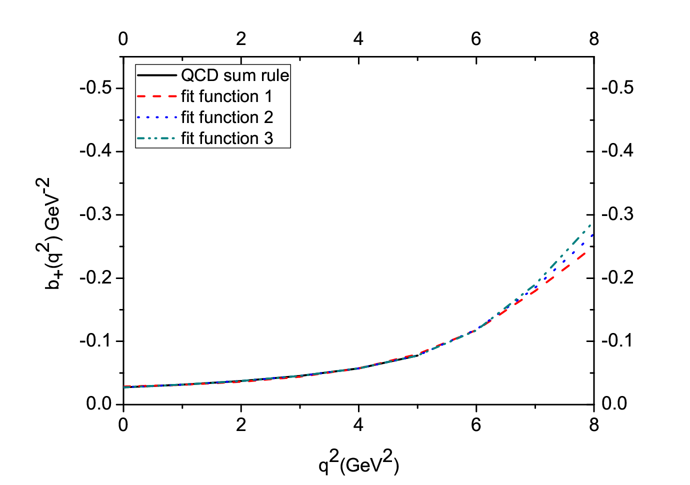
Figure 4: Left: b+b_{+}(q2q^{2}) as a function of q2q^{2} at M2=15​G​e​V2M^{2}=15GeV^{2}, M′2=10GeV2M^{\prime^{2}}=10GeV^{2}, s0=35​G​e​V2s_{0}=35GeV^{2} and s0′=9​G​e​V2s_{0}^{\prime}=9GeV^{2} . Right: b−b_{-}(q2q^{2}) as a function of q2q^{2} at M2=15​G​e​V2M^{2}=15GeV^{2}, M′2=10GeV2M^{\prime^{2}}=10GeV^{2}, s0=35​G​e​V2s_{0}=35GeV^{2} and s0′=9​G​e​V2s_{0}^{\prime}=9GeV^{2}.

Using the working regions for the continuum thresholds and Borel mass parameters as well as other input parameters we proceed to find the behavior of the form factors in terms of q2q^{2}. Our calculations show that the form factors are truncated at q2≃5​G​e​V2q^{2}\simeq 5GeV^{2}. In order to estimate the decay width of the B→D2∗​(2460)​ℓ​ν¯B\rightarrow D_{2}^{*}(2460)\ell\overline{\nu} transition, we have to obtain their fit functions in the whole physical region, mℓ2≤q2≤(mB−mD2∗)2m_{\ell}^{2}\leq q^{2}\leq(m_{B}-m_{D_{2}^{*}})^{2}. We find that the sum rules predictions for the form factors are well fitted to the following function:

f⁡(q2)=f0​exp⁡[c1​q2mf​i​t2+c2​(q2mf​i​t2)2]\displaystyle f(q^{2})=f_{0}\exp\Big[c_{1}\frac{q^{2}}{m_{fit}^{2}}+c_{2}\Big(\frac{q^{2}}{m_{fit}^{2}}\Big)^{2}\Big] (26)

where, the values of the parameters f0f_{0}, c1c_{1}, c2c_{2} and mf​i​t2m_{fit}^{2} are presented in Table 2. In the following, we will recall this parametrization as fit function 1. To compare our results with other parametrization, we also use the following fit functions to extrapolate the form factors to whole physical regions (see [15, 16, 17, 18]):

  • •

    fit function 2

    f⁡(q2)=f01−a⁡(q2mB2)+b​(q2mB2)2,\displaystyle f(q^{2})=\frac{f_{0}}{1-a(\frac{q^{2}}{m_{B}^{2}})+b(\frac{q^{2}}{m_{B}^{2}})^{2}}, (27)
  • •

    fit function 3

    f⁡(q2)=f0(1−q2mB2)​[1−A⁡(q2mB2)+B​(q2mB2)2],\displaystyle f(q^{2})=\frac{f_{0}}{\Big(1-\frac{q^{2}}{m_{B}^{2}}\Big)\Big[1-A(\frac{q^{2}}{m_{B}^{2}})+B(\frac{q^{2}}{m_{B}^{2}})^{2}\Big]}, (28)

where the parameters aa, bb, AA and BB and the values of corresponding form factors at q2=0q^{2}=0 are given in Tables 3 and 4, respectively.

f0abK⁡(q2)0.54±0.140.75±0.03−0.014±0.006b−​(q2)0.007±0.002​G​e​V−20.95±0.04−3.14±1.34b+​(q2)−0.03±0.01​G​e​V−21.41±0.06−4.63±2.05h⁡(q2)−0.010±0.003​G​e​V−21.27±0.050.058±0.002\begin{array}[]{|c|c|c|c|}\hline\cr\hline\cr&f_{0}&a&b\\ \hline\cr\mbox{$K(q^{2})$}&0.54\pm 0.14&0.75\pm 0.03&-0.014\pm 0.006\\ \hline\cr\mbox{$b_{-}(q^{2})$}&0.007\pm 0.002~GeV^{-2}&0.95\pm 0.04&-3.14\pm 1.34\\ \hline\cr\mbox{$b_{+}(q^{2})$}&-0.03\pm 0.01~GeV^{-2}&1.41\pm 0.06&-4.63\pm 2.05\\ \hline\cr\mbox{$h(q^{2})$}&-0.010\pm 0.003~GeV^{-2}&1.27\pm 0.05&0.058\pm 0.002\\ \hline\cr\hline\cr\end{array}
Table 3: Parameters appearing in the fit function 2 of the form factors.
f0ABK⁡(q2)0.54±0.14−0.15±0.060.31±0.03b−​(q2)0.007±0.002​G​e​V−2−0.36±0.16−7.72±0.86b+​(q2)−0.03±0.01​G​e​V−21.89±0.81−2.39±0.27h⁡(q2)−0.010±0.003​G​e​V−20.25±0.10−0.35±0.04\begin{array}[]{|c|c|c|c|}\hline\cr\hline\cr&f_{0}&A&B\\ \hline\cr\mbox{$K(q^{2})$}&0.54\pm 0.14&-0.15\pm 0.06&0.31\pm 0.03\\ \hline\cr\mbox{$b_{-}(q^{2})$}&0.007\pm 0.002~GeV^{-2}&-0.36\pm 0.16&-7.72\pm 0.86\\ \hline\cr\mbox{$b_{+}(q^{2})$}&-0.03\pm 0.01~GeV^{-2}&1.89\pm 0.81&-2.39\pm 0.27\\ \hline\cr\mbox{$h(q^{2})$}&-0.010\pm 0.003~GeV^{-2}&0.25\pm 0.10&-0.35\pm 0.04\\ \hline\cr\hline\cr\end{array}
Table 4: Parameters appearing in the fit function 3 of the form factors.

The dependences of form factors on q2q^{2} at different fixed values of auxiliary parameters are depicted in figures 3 and 4. These figures include the sum rules results (up to the truncated point) as well as the results obtained using the above mentioned three different fit functions. From these figures it is clear that, in the case of the form factors K⁡(q2)K(q^{2}), b+​(q2)b_{+}(q^{2}) and b−​(q2)b_{-}(q^{2}), all three fit functions reproduce the sum rules results up to the truncated point, however, we see small differences between the predictions of these fit functions at higher values of q2q^{2} except for the form factor K⁡(q2)K(q^{2}) that all fit functions give the same results. In the case of the form factor h⁡(q2)h(q^{2}), the parametrization 1 well fits to the sum rule result, but we see considerable differences of prediction of this parametrization with those of fit functions 2 and 3, especially at higher values of q2q^{2}.

Now we proceed to calculate the decay width and branching ratio of the process under consideration. The differential decay width for B→D2∗​(2460)​ℓ​ν¯B\rightarrow D_{2}^{*}(2460)\ell\overline{\nu} transition is obtained as [19]

d​Γd​q2\displaystyle\frac{d\Gamma}{dq^{2}} =\displaystyle= λ⁡(mB2,mD2∗2,q2)4​mD2∗2(q2−mℓ2q2)2λ⁡(mB2,mD2∗2,q2)​GF2​Vc​b2384​mB3​π3{12​q2[3mℓ2λ(mB2,mD2∗2,q2)[V0(q2)]2\displaystyle\frac{\lambda(m_{B}^{2},m_{D_{2}^{*}}^{2},q^{2})}{4m_{D_{2}^{*}}^{2}}\Big(\frac{q^{2}-m_{\ell}^{2}}{q^{2}}\Big)^{2}\frac{\sqrt{\lambda(m_{B}^{2},m_{D_{2}^{*}}^{2},q^{2})}G_{F}^{2}V_{cb}^{2}}{384m_{B}^{3}\pi^{3}}\Bigg\{\frac{1}{2q^{2}}\Bigg[3m_{\ell}^{2}\lambda(m_{B}^{2},m_{D_{2}^{*}}^{2},q^{2})[V_{0}(q^{2})]^{2} (29)
+\displaystyle+ (mℓ2+2q2)|12​mD2∗[(mB2−mD2∗2−q2)(mB−mD2∗)V1(q2)−λ⁡(mB2,mD2∗2,q2)mB−mD2∗V2(q2)]|2]\displaystyle(m_{\ell}^{2}+2q^{2})\Big|\frac{1}{2m_{D_{2}^{*}}}\Big[(m_{B}^{2}-m_{D_{2}^{*}}^{2}-q^{2})(m_{B}-m_{D_{2}^{*}})V_{1}(q^{2})-\frac{\lambda(m_{B}^{2},m_{D_{2}^{*}}^{2},q^{2})}{m_{B}-m_{D_{2}^{*}}}V_{2}(q^{2})\Big]\Big|^{2}\Bigg]
+\displaystyle+ 23(mℓ2+2q2)λ(mB2,mD2∗2,q2)[|A⁡(q2)mB−mD2∗−(mB−mD2∗)​V1​(q2)λ⁡(mB2,mD2∗2,q2)|2\displaystyle\frac{2}{3}(m_{\ell}^{2}+2q^{2})\lambda(m_{B}^{2},m_{D_{2}^{*}}^{2},q^{2})\Bigg[\Big|\frac{A(q^{2})}{m_{B}-m_{D_{2}^{*}}}-\frac{(m_{B}-m_{D_{2}^{*}})V_{1}(q^{2})}{\sqrt{\lambda(m_{B}^{2},m_{D_{2}^{*}}^{2},q^{2})}}\Big|^{2}
+\displaystyle+ |A⁡(q2)mB−mD2∗+(mB−mD2∗)​V1​(q2)λ⁡(mB2,mD2∗2,q2)|2]},\displaystyle\Big|\frac{A(q^{2})}{m_{B}-m_{D_{2}^{*}}}+\frac{(m_{B}-m_{D_{2}^{*}})V_{1}(q^{2})}{\sqrt{\lambda(m_{B}^{2},m_{D_{2}^{*}}^{2},q^{2})}}\Big|^{2}\Bigg]\Bigg\},

where

A⁡(q2)\displaystyle A(q^{2}) =\displaystyle= −(mB−mD2∗)​h​(q2),\displaystyle-(m_{B}-m_{D_{2}^{*}})h(q^{2}),
V1​(q2)\displaystyle V_{1}(q^{2}) =\displaystyle= −K⁡(q2)mB−mD2∗,\displaystyle-\frac{K(q^{2})}{m_{B}-m_{D_{2}^{*}}},
V2​(q2)\displaystyle V_{2}(q^{2}) =\displaystyle= (mB−mD2∗)​b+​(q2),\displaystyle(m_{B}-m_{D_{2}^{*}})b_{+}(q^{2}),
V0​(q2)\displaystyle V_{0}(q^{2}) =\displaystyle= mB−mD2∗2​mD2∗​V1​(q2)−mB+mD2∗2​mD2∗​V2​(q2)−q22​mD2∗​b−​(q2),\displaystyle\frac{m_{B}-m_{D_{2}^{*}}}{2m_{D_{2}^{*}}}V_{1}(q^{2})-\frac{m_{B}+m_{D_{2}^{*}}}{2m_{D_{2}^{*}}}V_{2}(q^{2})-\frac{q^{2}}{2m_{D_{2}^{*}}}b_{-}(q^{2}),
λ⁡(a,b,c)\displaystyle\lambda(a,b,c) =\displaystyle= a2+b2+c2−2​a​b−2​a​c−2​b​c.\displaystyle a^{2}+b^{2}+c^{2}-2ab-2ac-2bc. (30)

After performing integration over q2q^{2} in Eq. (29) in the interval mℓ2≤q2≤(mB−mD2∗)2m_{\ell}^{2}\leq q^{2}\leq(m_{B}-m_{D_{2}^{*}})^{2}, we obtain the total decay widths and branching ratios for all leptons and three different fit functions presented in Table 5. The errors in the results belong to the uncertainties in determination of the working regions for the auxiliary parameters as well as errors in the other input parameters. From this Table, it is clear that, for the ee and μ\mu channels, all fit functions give roughly the same results. In the case of τ\tau, the fit functions 2 and 3 have approximately the same predictions, but they give results roughly %38 smaller than that of the fit function 1. As it is expected, the values for the branching ratios in the cases of ee and μ\mu are very close to each other for all fit functions. The orders of branching fractions show that this transition can be detected at LHCb for all lepton channels. Note that there are experimental data on the products of branching fractions for the decay chain ℬ⁡(B→D2∗​ℓ​ν¯)​ℬ​(D2∗→D​π){\cal{B}}(B\rightarrow D_{2}^{*}\ell\overline{\nu}){\cal{B}}(D_{2}^{*}\rightarrow D\pi) provided by Belle [20] and BaBar [21, 22] Collaborations:

ℬ(B+→D¯2∗ℓ′+ν¯ℓ′)ℬ(D¯2∗→Dπ)\displaystyle{\cal{B}}(B^{+}\rightarrow\overline{D}_{2}^{*}\ell^{{}^{\prime}+}\overline{\nu}_{\ell^{\prime}}){\cal{B}}(\overline{D}_{2}^{*}\rightarrow D\pi) =\displaystyle= 2.2±0.3±0.4Belle [20],\displaystyle 2.2\pm 0.3\pm 0.4~~~~~~~~~~\mbox{Belle \cite[cite]{[\@@bibref{}{belle}{}{}]}},
ℬ(B+→D¯2∗ℓ′+ν¯ℓ′)ℬ(D¯2∗→Dπ)\displaystyle{\cal{B}}(B^{+}\rightarrow\overline{D}_{2}^{*}\ell^{{}^{\prime}+}\overline{\nu}_{\ell^{\prime}}){\cal{B}}(\overline{D}_{2}^{*}\rightarrow D\pi) =\displaystyle= 1.4±0.2±0.2BaBar [21, 22].\displaystyle 1.4\pm 0.2\pm 0.2~~~~~~~~~~\mbox{BaBar \cite[cite]{[\@@bibref{}{babar1,babar2}{}{}]}}. (31)

where l′=el^{\prime}=e or μ\mu. Considering the recent experimental progress especially at LHC we hope we will have experimental data on the branching fraction of the semileptonic B→D2∗​(2460)​ℓ​ν¯B\rightarrow D_{2}^{*}(2460)\ell\overline{\nu} transition in near future, comparison of which with the results of the present work can give more information about the nature and internal structure of the D2∗​(2460)D_{2}^{*}(2460) tensor meson.

 fit function 1Γ⁡(G​e​V)B​rB→D2∗​(2460)​τ​ν¯τ(6.52±2.20)×10−17(0.16±0.06)×10−3B→D2∗​(2460)​μ​ν¯μ(4.04±1.18)×10−16(1.00±0.29)×10−3B→D2∗​(2460)​e​ν¯e(4.05±1.19)×10−16(1.01±0.30)×10−3 fit function 2Γ⁡(G​e​V)B​rB→D2∗​(2460)​τ​ν¯τ(4.09±1.28)×10−17(0.10±0.03)×10−3B→D2∗​(2460)​μ​ν¯μ(4.06±1.26)×10−16(1.01±0.32)×10−3B→D2∗​(2460)​e​ν¯e(4.08±1.28)×10−16(1.02±0.32)×10−3 fit function 3Γ⁡(G​e​V)B​rB→D2∗​(2460)​τ​ν¯τ(4.80±1.60)×10−17(0.12±0.04)×10−3B→D2∗​(2460)​μ​ν¯μ(4.18±1.32)×10−16(1.04±0.34)×10−3B→D2∗​(2460)​e​ν¯e(4.20±1.32)×10−16(1.05±0.34)×10−3\begin{array}[]{|c|c|c|}\hline\cr\hline\cr\mbox{ fit function 1}&\Gamma(GeV)&Br\\ \hline\cr\mbox{$B\rightarrow D_{2}^{*}(2460)\tau\overline{\nu}_{\tau}$}&(6.52\pm 2.20)\times 10^{-17}&(0.16\pm 0.06)\times 10^{-3}\\ \hline\cr\mbox{$B\rightarrow D_{2}^{*}(2460)\mu\overline{\nu}_{\mu}$}&(4.04\pm 1.18)\times 10^{-16}&(1.00\pm 0.29)\times 10^{-3}\\ \hline\cr\mbox{$B\rightarrow D_{2}^{*}(2460)e\overline{\nu}_{e}$}&(4.05\pm 1.19)\times 10^{-16}&(1.01\pm 0.30)\times 10^{-3}\\ \hline\cr\hline\cr\mbox{ fit function 2}&\Gamma(GeV)&Br\\ \hline\cr\mbox{$B\rightarrow D_{2}^{*}(2460)\tau\overline{\nu}_{\tau}$}&(4.09\pm 1.28)\times 10^{-17}&(0.10\pm 0.03)\times 10^{-3}\\ \hline\cr\mbox{$B\rightarrow D_{2}^{*}(2460)\mu\overline{\nu}_{\mu}$}&(4.06\pm 1.26)\times 10^{-16}&(1.01\pm 0.32)\times 10^{-3}\\ \hline\cr\mbox{$B\rightarrow D_{2}^{*}(2460)e\overline{\nu}_{e}$}&(4.08\pm 1.28)\times 10^{-16}&(1.02\pm 0.32)\times 10^{-3}\\ \hline\cr\hline\cr\mbox{ fit function 3}&\Gamma(GeV)&Br\\ \hline\cr\mbox{$B\rightarrow D_{2}^{*}(2460)\tau\overline{\nu}_{\tau}$}&(4.80\pm 1.60)\times 10^{-17}&(0.12\pm 0.04)\times 10^{-3}\\ \hline\cr\mbox{$B\rightarrow D_{2}^{*}(2460)\mu\overline{\nu}_{\mu}$}&(4.18\pm 1.32)\times 10^{-16}&(1.04\pm 0.34)\times 10^{-3}\\ \hline\cr\mbox{$B\rightarrow D_{2}^{*}(2460)e\overline{\nu}_{e}$}&(4.20\pm 1.32)\times 10^{-16}&(1.05\pm 0.34)\times 10^{-3}\\ \hline\cr\hline\cr\end{array}
Table 5: Numerical results for the decay widths and branching ratios at different lepton channels for different fit functions.

At the end of this section we would like to calculate the ratio of the branching fraction in the case of τ\tau to that of the ee or μ\mu. From our calculations we obtain that

ℛ=B→D2∗​(2460)​τ​ν¯τB→D2∗​(2460)​ℓ′​ν¯ℓ′={0.16±0.04fit function 1,0.10±0.02fit function 2,0.11±0.02fit function 3.\displaystyle{\cal R}=\frac{B\rightarrow D_{2}^{*}(2460)\tau\overline{\nu}_{\tau}}{B\rightarrow D_{2}^{*}(2460)\ell^{\prime}\overline{\nu}_{\ell^{\prime}}}=\left\{\begin{array}[]{c}0.16\pm 0.04~~~~\mbox{fit function 1},\\ 0.10\pm 0.02~~~~\mbox{fit function 2},\\ 0.11\pm 0.02~~~~\mbox{fit function 3}.\end{array}\right.

As we previously mentioned the SM predictions in the BB to pseudoscalar and vector charmed mesons deviate at the level of 3.4σ~\sigma from the experimental data. Our result on ℛ{\cal R} in the case of tensor charmed current can be checked in future experiments. Comparison of the experimental data with the result of this work will illustrate whether these anomalous in the pseudoscalar and vector channels exist also in the tensor channel or not.

References

  • [1] P. del Amo Sanchez et al. [BABAR Collaboration], Phys. Rev. D 82, 111101 (2010).
  • [2] D. Becirevic, B. Blossier, A. Gerardin, A. Le Yaouanc, F. Sanfilippo, arXiv:1301.7336 [hep-ph].
  • [3] J. Segovia, C. Albertus, D.R. Entem, F. Fernandez, E. Hernandez, M.A. Perez-Garcia, Phys. Rev. D 84, 094029 (2011).
  • [4] F. De Fazio, PoS HQL2012, 001 (2012).
  • [5] P. Colangelo, F. De Fazio, F. Giannuzzi and S. Nicotri, Phys. Rev. D 86, 054024 (2012).
  • [6] M. A. Shifman, A. I. Vainshtein and V. I. Zakharov, Nucl. Phys. B 147, 385 (1979).
  • [7] J. P. Lees et al. [BaBar Collaboration], Phys. Rev. Lett. 109, 101802 (2012).
  • [8] S. Fajfer, J. F. Kamenik and I. Nisandzic, Phys. Rev. D 85, 094025 (2012).
  • [9] P. Biancofiore, P. Colangelo, F. De Fazio, arXiv:1302.1042 [hep-ph].
  • [10] J. Beringer et al., (Particle Data Group) Phys. Rev. D 86, 010001, (2012).
  • [11] H. Sundu, K. Azizi, Eur. Phys. J. A 48 (2012) 81.
  • [12] H. Na, C. J. Monahan, C. T. H. Davies, R. Horgan, G. P. Lepage, J. Shigemitsu, Phys. Rev. D 86, (2012) 034506.
  • [13] B. L. Ioffe, Prog. Part. Nucl. Phys. 56, 232 (2006).
  • [14] H. G. Dosch, M. Jamin and S. Narison, Phys. Lett. B 220, 251 (1989); V. M. Belyaev, B. L. Ioffe, Sov. Phys. JETP, 57, 716 (1982).
  • [15] W. Wang, Phys. Rev.D 83, 014008 (2011).
  • [16] R.-H. Li, C.-D. Lü, W. Wang, Phys. Rev. D 83, 034034 (2011).
  • [17] C.-D. Lü, W. Wang, Phys. Rev. D 85, 034014 (2012).
  • [18] H.-Y. Cheng, C.-K. Chua, C.-W. Hwang, Phys. Rev. D 69, 074025 (2004).
  • [19] X.-X. Wang, W. Wang and C.-D. Lü, Phys. Rev. D 79, 114018, (2009).
  • [20] D. Liventsev et al. (Belle Collaboration), Phys. Rev. D 77, 091503 (2008).
  • [21] B. Aubert et al. (BaBar Collaboration), Phys. Rev. Lett. 101, 261802 (2008).
  • [22] B. Aubert et al. (BaBar Collaboration), Phys. Rev. Lett. 103, 051803 (2009).