Matter effects on binary neutron star waveforms
Abstract
Using an extended set of equations of state and a multiple-group multiple-code collaborative effort to generate waveforms, we improve numerical-relativity-based data-analysis estimates of the measurability of matter effects in neutron-star binaries. We vary two parameters of a parameterized piecewise-polytropic equation of state (EOS) to analyze the measurability of EOS properties, via a parameter that characterizes the quadrupole deformability of an isolated neutron star. We find that, to within the accuracy of the simulations, the departure of the waveform from point-particle (or spinless double black-hole binary) inspiral increases monotonically with , and changes in the EOS that did not change are not measurable.
We estimate with two methods the minimal and expected measurability of in second- and third-generation gravitational-wave detectors. The first estimate, using numerical waveforms alone, shows two EOS which vary in radius by km are distinguishable in mergers at 100 Mpc. The second estimate relies on the construction of hybrid waveforms by matching to post-Newtonian inspiral, and estimates that the same EOS are distinguishable in mergers at 300 Mpc. We calculate systematic errors arising from numerical uncertainties and hybrid construction, and we estimate the frequency at which such effects would interfere with template-based searches.
I Introduction
Substantial uncertainty remains in the equation of state (EOS) of cold matter above nuclear density. While recent analyses of X-ray bursts and thermal emission from quiescent low-mass X-ray binaries [1, 2, 3, 4, 5, 6, 7] constrain simultaneously the mass and radius of neutron stars in X-ray binaries, placing limits on allowed EOS, such measurements depend on burst and atmosphere models. In contrast, observations of gravitational waves from binary inspiral provide a model-independent way to simultaneously measure the mass and radius of neutron stars in double neutron-star and black-hole neutron-star binaries.
The detection of a gravitational wave from an inspiraling binary will determine mass parameters from the early inspiral [8]. Strong signals may also constrain additional parameters that characterize the EOS. For widely separated neutron-star pairs, EOS effects will be minuscule; however, binary systems drawn together by the loss of orbital angular momentum to gravitational radiation will exhibit increasing tidal interactions through the late stage of binary inspiral, up to tidal disruption or merger. The effects of tidal interactions imprint an EOS signature on the gravitational waveform of the merger of the neutron stars.
The rate of binary neutron star mergers is uncertain, but it is reasonable to expect that Advanced LIGO[9] will detect several events per year [10]. In fact, over several years of operation, there appears to be a good chance that a strong signal, with signal-to-noise ratio (SNR) above 30, will be detected.
Neutron-star pairs in binary systems produce mutual tidal stresses that deform the metric around the stars in a manner prescribed by the EOS, via a parameter we refer to as the tidal deformability, , defined in Eq. (1) below. This parameter describes the degree to which a local metric suffers quadrupolar deformations when in the tidal field of a companion, and scales as the fifth power of the neutron-star radius, . The tidal interaction between two stars in a binary system alters both the binding energy of the system and the gravitational-wave energy flux [11, 12, 13], and in turn changes the phase evolution of the gravitational waveform. When the stars are sufficiently far apart, the phase evolution may be obtained from a detailed balance of energy through a sequence of orbits. This approach describes the secular evolution of the binary system orbit under energy loss to gravitational radiation (and distortion of the companions) and is valid while the evolution is slow and the motions are not too relativistic. Analysis using analytic models suggests that tidal effects may be measurable using Advanced LIGO [11, 14, 15], but only if the model can be extended to the late, high-frequency stages of inspiral.
Large tidal effects on the merger of binary neutron star systems terms have been observed in numerical simulations of late inspiral [16, 17, 18, 19, 20]. Additional information is also present in the frequencies of neutron-star normal modes after the merger, should the EOS be stiff enough to support a hypermassive neutron star [21, 22, 23]. In this paper, we incorporate a wider range of EOS than previous work, with systematic parameter variation that allows us to explicitly estimate how EOS parameters will be constrained; we show that, to within the accuracy of our simulations, the parameter can also be used to characterize the merger of binary neutron stars.
While numerical-relativity efforts can simulate binary coalescence during the highly dynamical phase at the endpoint of binary inspiral, there are additional challenges in determining the slow inspiral motion: simulating the length-scales and time-scales of widely separated binary systems whose orbital decay occurs over many cycles is computationally expensive, and the resolution must be sufficiently high that the numerical scheme conserves angular momentum and energy with enough accuracy that the relatively small gravitational radiation dominates. However, if high-quality numerical simulations extend into the region in which a given post-Newtonian or other analytic approximation is valid, joining the post-Newtonian waveform to the numerical waveform at a point when both waveforms are deemed accurate will yield a complete hybrid waveform for the binary system, which includes both inspiral tidal effects and other hydrodynamic effects that occur during coalescence. Hybrid waveforms can be used to better measure the EOS-dependent properties of a neutron star. The measurement will be limited not only by statistical errors arising from the fact that the gravitational-wave signal must be extracted from detector noise, but also by systematic errors arising from modeling errors in the analytic inspiral, the numerical simulations, and ambiguities in the process of joining them together.
We also explore an alternative scenario: If systematic errors arising from hybrid waveforms are intractable, it is possible to use only numerical simulations of the late inspiral, which are robust, to estimate structural parameters of the neutron star. The measurability of the tidal deformability suffers in such an approach because the unknown time and phase of the numerical waveform relative to the time and phase of post-Newtonian models of the early inspiral must be marginalized over. However, we show that we are still able to constrain the tidal deformability of neutron stars in binary neutron-star systems, using current numerical simulations, even if hybrid waveforms cannot be constructed.
Our results are derived from data produced by two independent numerical-relativity codes: SACRA [24] and Whisky [25, 26, 27]. This has the advantages of checking the actual numerical differences due to different implementations of the equations (Einstein equations, relativistic-hydrodynamics equations) and of understanding if and how much such differences are relevant to gravitational-wave detection and analysis.
We use a spacelike signature and a system of units in which c = G = 1. Greek indices are taken to run from 0 to 3, Latin indices from 1 to 3, and we adopt the standard convention for the summation over repeated indices.
II Generation of Waveforms
II.1 EOS variation
We specify EOS candidates in the framework of [28, 16]: A fixed crust EOS is joined to a core EOS that we vary using a piecewise polytrope scheme. Currently we consider a single core region, but we vary independently two parameters: the adiabatic index of the core and the overall pressure scale at a fiducial density g/cm3. Following the notation of [16, 29], we categorize the EOS by the pressure scale: From high pressure to low pressure we use 2H, H, HB, and B. The adiabatic index variation is indicated by one or more occurrences of a lower case s: H (no s) has , Hs has , Hss has . Eight EOSs (2H,H, HB, B, Bs, Bss, HBs, HBss) were simulated using both the Whisky and SACRA codes, at multiple resolutions and at different initial stellar separations (see Sec. II.2.1). EOS parameters are summarized in Table 1.
| EOS | |||||||
|---|---|---|---|---|---|---|---|
| 2H | 34.9036 | 3.0 | 15.23 | 0.131 | 10.97 | 4.713 | 2325 |
| H | 34.5036 | 3.0 | 12.28 | 0.162 | 2.866 | 3.603 | 607.3 |
| HB | 34.4036 | 3.0 | 11.61 | 0.172 | 1.992 | 3.350 | 422.0 |
| B | 34.3036 | 3.0 | 10.96 | 0.182 | 1.362 | 3.105 | 288.7 |
| Bs | 34.3036 | 2.7 | 10.74 | 0.186 | 1.075 | 2.961 | 227.7 |
| Bss | 34.3036 | 2.4 | 10.27 | 0.194 | 0.6695 | 2.694 | 141.9 |
| HBs | 34.4036 | 2.7 | 11.58 | 0.172 | 1.770 | 3.275 | 376.9 |
| HBss | 34.4036 | 2.4 | 11.45 | 0.174 | 1.421 | 3.131 | 301.1 |
For a given neutron-star mass, each EOS can be identified by two useful macroscopic characteristic quantities, and : is the stellar radius of an isolated nonrotating neutron star and
| (1) |
is the dimensionless quadrupole tidal deformability ( is the quadrupole Love number). These parameters are tabled for the current models in Table 1. Recent analysis of neutron-star matter properties compatible with modern nuclear theory [30] suggests that the radius of the 2H model is unrealistically large, and the neutron-star mass measurement of 2.0 [31] rules out the “s” EOSs. Current astrophysical constraints [1, 2, 3, 4, 5, 6] further favor EOS H and HB. However, we consider this range useful for a parameter study.
At leading order in the separation of the stars, determines the departure of the asymptotic metric from spherical symmetry and the departure of the waveform phase evolution from its point-particle form. Our results imply that effectively determines the waveform’s departure from point-particle (or nonspinning BH-BH) inspiral even for the late inspiral.
Fig. 2 (provided by B. D. Lackey) shows contours of constant and for 1.35 stars in the EOS space. Our simulations suggest that the contours in the EOS parameter space of constant departure of the waveform from point-particle inspiral coincide with similar accuracy with these contours of constant , but the range of high-resolution runs is not yet large enough for a quantitative conclusion.
II.2 Numerical simulations
Here we give only a brief overview of the codes, while we refer the reader to previous articles for more details [32, 24, 25, 26, 33, 34].
II.2.1 Initial data
The initial configurations for our simulations are produced using the numerical code of [35, 36, 37], based on the multidomain spectral-method library, LORENE. LORENE was originally written by the Meudon relativity group and is publicly available [38]. We have added a new method to treat the piecewise polytropic EOS of Sec. II.1, which is used in [32] for detailed study of quasiequilibrium sequences with such EOS.
The total mass is fixed to be at infinite separation. We consider equal-mass binaries. The initial data are prepared for two different orbital angular velocities, and 0.0221, where denotes the initial orbital angular velocity, subsequently labelled by “I188” and “I221”. Nine models are prepared for our simulations, varying the EOS and orbital angular velocity for fixed total mass. Some of the physical quantities of the initial configurations are reported in Table 2.
| Mass () | |||||||||||
|---|---|---|---|---|---|---|---|---|---|---|---|
| EOS | Whisky | SACRA | |||||||||
| 2H I188 | |||||||||||
| HB I188 | |||||||||||
| B I221 | |||||||||||
| Bss I221 | |||||||||||
II.2.2 Overview of evolution codes
Both the SACRA and Whisky codes evolve the Einstein equations in the Baumgarte-Shapiro-Shibata-Nakamura formalism [39, 40, 41, 42]. For the Whisky simulations, the Einstein equations are solved using the CCATIE code, a three-dimensional finite-differencing code based on the Cactus Computational Toolkit [43]. A detailed presentation of the CCATIE code and of its convergence properties has been presented in [33]. For tests and details on SACRA, see [24].
The gauges are specified in terms of the standard Arnowitt-Deser-Misner (ADM) lapse function, , and shift vector, [44]. We evolve the lapse according to the “” slicing condition [45]:
| (2) |
The shift is evolved using the hyperbolic -driver condition [46]
| (3) | |||||
| (4) |
where is an auxiliary variable and is a parameter that acts as a damping coefficient. We set or , in units of , for Whisky and SACRA respectively.
Both codes adopt a flux-conservative formulation of the hydrodynamics equations [47, 48, 49], in which the set of conservation equations for the stress-energy tensor and for the matter current density (where is the pressure, is the rest-mass density, is the specific internal energy, is the specific enthalpy, is the four-velocity and is the inverse metric), namely and , are written in a hyperbolic, first-order, flux-conservative form of the type
| (5) |
where and are the flux vectors and source terms, respectively [50]. The EOS closes the system by relating pressure, rest-mass density, and internal-energy density.
The system written in conservative form is solved with high-resolution shock-capturing methods, in several variants for both codes. For the simulations of this work, both codes employ 3rd order piecewise-parabolic method (PPM) [51] reconstruction, but SACRA used Kurganov-Tadmor’s central scheme [52] for Riemann solvers, while Whisky [53] use the Marquina flux formula. The details of the differences in the implementations of the Einstein and hydrodynamics equations in the two codes are described in [54], which contains also convergence tests and the description of the differences in the implementations of adaptive mesh refinement [55, 24].
| Refinement | Moving | Finest Grid (km) | Coarsest Grid (km) | |||
|---|---|---|---|---|---|---|
| Model | Levels | Levels | Spacing | Extent | Spacing | Outer Boundary |
| B Whisky R141 I221 (HR) | 2 | |||||
| B Whisky R177 I221 (MR) | 2 | |||||
| B Whisky R221 I221 (LR) | 2 | |||||
| B SACRA R157 I221 (HR) | 4 | |||||
| B SACRA R174 I221 (MR) | 4 | |||||
| B SACRA R202 I221 (LR) | 4 | |||||
For the highest-resolution runs with Whisky, the spacing of the finest of the six grid levels is and the spacing in the wave zone (the coarsest grid) is . The finest grid always covers the whole stars. The outer boundary is located at about .
For the runs with SACRA, the computational domain comprises seven grid levels, with finest grid resolution and with spacing in the wave zone (the coarsest grid) km for the highest-resolution runs. The finest grid covers the stellar radius completely (the boundary of the finest grid is at of the stellar radius). The radius of the outer boundary is about .
The properties of the grids adopted in the simulations with the two codes are summarized in Table 3. In general, we use a naming convention to label results for a given numerical simulation, e.g. “HB Whisky R141 I221”, which summarizes the EOS (HB), the code (Whisky), the resolution of the finest grid in meters (141), and the initial orbital angular velocity imposed for building the initial data expressed as (221).
II.3 Waveform extraction
This work is concerned primarily with the gravitational waveform extracted from the simulation, rather than the underlying density or pressure distributions, so we describe in some detail the gravitational-wave methods employed.
Both codes compute the gravitational waveforms using the Newman-Penrose formalism [56], which provides a convenient representation for a number of radiation-related quantities as spin-weighted scalars. In particular, the curvature scalar
| (6) |
is defined as a particular component of the Weyl curvature tensor projected onto a given null frame and can be identified with the gravitational radiation field if a suitable frame is chosen at the extraction radius. In practice, we define an orthonormal basis in the three-space , centered on the Cartesian origin and oriented with poles along . The normal to the slice defines a timelike vector , from which we construct the null frame
| (7) |
We then calculate via a reformulation of (6) in terms of ADM variables on the slice [57]:
| (8) |
where
| (9) |
and is the Levi-Civita symbol. The gravitational-wave polarization amplitudes and are then related to by time integrals [58]:
| (10) |
where the double overdot stands for the second-order time derivative. Care is needed when performing such time integrals [59, 18, 60]. In SACRA, they are computed with the fixed-frequency integration method [61].
For the extraction of the gravitational-wave signal, each code implements a second independent method that is based on expressions involving the gauge-invariant metric perturbations of a spherically symmetric background spacetime [62]. The wave data obtained in this way give results compatible with those obtained with the Newman-Penrose formalism and are not reported here.
We use only the mode in this work. For the equal-mass cases considered, other modes are much smaller. The waveform is analyzed as a function of retarded time where is the ADM mass of the system at the initial time of the simulation.
We will use the complex combination of the extracted polarizations
| (11) |
in further analysis. Some relevant quantities of a detected signal can be calculated for either polarization and in this paper we will always show the average result for both polarizations.
An instantaneous frequency is extracted by taking the time derivative of the phase of the complex waveform. The total accumulated phase is reconstructed by integrating the instantaneous frequency in subsequent phase plots.
The physical system simulated is the same under translations by arbitrary parameters, and , which describe, respectively, the time of the start of the simulation relative to some reference time and the initial phase of the simulation relative to some reference phase. When comparing two waveforms, these free parameters amount to a relative time shift and phase shift between the waveforms. For the numerical waveforms with the same initial separation, one can take the time and phase to be zero at the retarded time corresponding to the start of the simulation. For simulations of EOS B, detailed comparison results between SACRA and Whisky are presented in [54].
II.4 Common structure of waveforms
In order to compare simulations with different starting points, or to remove artificial effects of initial data, an alternate alignment procedure is required. In fully realistic binary simulations, as in the binary black hole case, the merger is the simplest reference point for waveform comparison. With finite resolution, numerical dissipation may cause angular momentum to be artificially lost during the evolution, increasing the rate of orbital decay during the secular inspiral in a way that may mimic the tidal effects that are being studied here. Evolutions with different resolutions of the same initial data tend to diverge from one another when they are aligned to start at the same time and with the same phase. However, this direct comparison overemphasizes differences that are less relevant to our purposes, as small differences in phase accumulation in the early, low-frequency regime will induce a corresponding time shift which translates to a large phase difference in the later high-frequency cycles. During the late stages of binary coalescence, which are driven by dynamical effects, the effects of numerical dissipation are less significant. Comparable resolution-dependent features of binary-black hole simulations motivated alignment of waveforms at merger in comparisons such as those described in Hannam et al. [63].
We will align multiple waveforms with the same EOS so that all waveforms have the same time and phase when they reach their maximum amplitude (Fig. 3 and Fig. 5), which also allows the comparison of waveforms with different initial separations. The numerical waveforms have residual oscillations in their amplitude as they approach the peak, so we smooth this by taking a moving average of the amplitude over a range of 0.5 ms before finding the maximum amplitude.
Different simulations of the same physical system, including those with differing initial data, agree well through the last orbits when the waveforms are compared this way, which we consider a strong indication that the dynamical phase is being reliably simulated. We then estimate numerical inaccuracies on the waveforms relative to the peak amplitude time to determine how much of the inspiral we will use in subsequent analysis.
Looking at a set of waveforms, we find a common structure that is seen for each EOS in Fig. 3. As the neutron stars spiral toward each other, at some point there is a transition from an inspiral phase to a merger or coalescence phase, indicated by a maximum in the amplitude at the end of the inspiral phase. The retarded time of the peak amplitude corresponds roughly to the impact of the two stars, after which shocks form and thermal and other effects are expected to contribute to the waveform [64, 65, 66, 67, 68].
Somewhat surprisingly, we find that the parameter effectively characterizes properties at this peak amplitude. Fig. 4 shows the frequency at peak amplitude as a function of both compactness, the dimensionless ratio for an individual star, and for the individual stars. We find that the frequency varies more smoothly with than with radius or compactness; a linear fit of as a function of is displayed. This may be an analogous relation to those explored in [69].
The instantaneous frequency of the gravitational waveform continues to increase for a short time after the peak amplitude is reached, as the stars coalesce. A minimum in the gravitational wave amplitude follows, around which the instantaneous frequency is not well defined and may spike upwards or downwards.
After this point, the qualitative waveform behavior depends strongly on the EOS: For EOSs with higher pressure at the relevant densities, a differentially rotating hypermassive object may be supported, producing a quasi-periodic post-merger oscillation waveform [34, 70]. This can last for tens of milliseconds before the remnant collapses to a black hole [71]. EOSs with lower pressure, conversely, collapse quickly to black holes and have short post-coalescence signals at roughly ringdown frequency, though of lower amplitude than their binary black hole counterparts. The exact frequency and amplitude of this signal varies with the EOS.
The differences in phase evolution of different waveforms with the same EOS are shown relative to a well-resolved reference waveform in Fig. 5. We note that the difference in the finest resolution between simulations explains much of the phase difference for all EOS; difference between initial separation (and resulting differences in eccentricity at merger) have relatively small effects at these resolutions.
Furthermore, we note that the magnitude of the phase differences stemming from difference in resolution depends on the EOS: more compact stars require higher resolution to give comparably small phase error. This makes a quantitative comparison of resolution effects on waveforms with different EOSs more challenging. For this analysis, we use a simplified procedure: examining the merger-aligned waveforms, we estimate which of the given waveforms are sufficiently resolved by current simulations by comparison with the highest resolution available. We will consider only waveforms which differ from the highest resolution simulation by less than 0.5 radians over the last 15 ms before the peak amplitude is reached. The systematic error resulting from this level of phase error is calculated for the various measurability estimates in subsequent sections.
II.4.1 Detectors considered and Fourier-amplitude spectra
For the merger of binary neutron stars, only detector configurations with good high-frequency sensitivity will give useful constraints; broadband configurations have previously been shown to compare favorably to narrowband configurations tuned for high frequency sensitivity in distinguishing matter effects [28]. In this work, we choose the zero-detuning high-power Advanced LIGO configuration [72], and the ET-D Einstein telescope configuration [73].
We use a reference effective distance of to present results in this paper. The effective distance of a binary system is same as the true distance of the system if it is optimally oriented (face-on) and optimally located (directly above or below the detector) and is greater than the true distance otherwise. The amplitude of a signal is inversely proportional to its effective distance.
The rate of signals with Mpc or smaller can be estimated by comparing this to the fiducial Advanced LIGO horizon distance—the effective distance of a detectable signal—of 445 Mpc for NS-NS inspirals [10]. Within this horizon, we expect roughly 40 (0.4–400) detectable inspirals per year. Since rate scales with for sufficiently large distances, we expect of the detected signals to be as strong or stronger than our reference signal, making it a plausible “loudest” signal over a few years of observation with realistic event rates. However, we will also consider how our results scale to other values of and the constraints that weaker signals would place on the EOS in the sections to follow.
The estimates in this paper conservatively use only a single Advanced LIGO detector. However, two detectors are being upgraded in the United States [9], a third is planned in India [75], and an upgrade of comparable high-frequency sensitivity is underway for Virgo [76] in Italy; finally, a Japanese detector, KAGRA [77] is under construction, although KAGRA’s sensitivity curve is shifted slightly to lower frequency. A multiple-detector network will provide additional discriminatory power, reducing the statistical (though not the systematic) errors from those estimated in this work.
In Fig. 6, we compare the amplitude of the simulated waveforms as a function of frequency for each EOS to the strain sensitivity of the detectors. Results of simulations with different codes, resolutions, and initial separations are overlaid for each physically distinct inspiral. The amplitude of the Fourier transform is an incomplete representation of the waveform; similarities in amplitude do not necessarily reflect similarities in phase evolution and can camouflage slow secular phase contributions that decohere two waveforms. However, the amplitude has the advantage of being independent of shifts in time and phase between two waveforms.
The consistent change of the spectra as (and radius) increase shows the effect of the EOS on the waveform at high frequency. While insufficient resolution (e.g., the dotted EOS B curve) may result in artificially low amplitudes at lower frequencies, varying resolutions tend to agree in amplitude before the systems transition to merger the characteristic frequency of the peak amplitude. Note that the spectra of more compact neutron stars (EOS B, HBss, and Bss) follow black-hole inspiral to higher frequencies, but have significantly different merger/ringdown amplitudes.
The finite length of the numerical waveforms leads to a drop-off in the amplitude at low frequencies. In the lower-resolution runs, resolution-dependent dissipation in early cycles also results in a decrease in the Fourier amplitude at lower frequencies relative to higher-resolution waveforms with the same initial separation.
II.5 Post-merger oscillations
Post-merger oscillations dominate the gravitational-wave emission from hypermassive neutron-star remnant formed after the merger. They are stronger, lower-frequency, and longer-lasting than the ringdown of a black hole formed in prompt collapse. The amplitude of the post-merger oscillation spectra are shown in Fig. 7. If strong enough, the high-frequency signals could be independently detected by a search triggered by the inspiral, and could constrain a combination of cold [78] and hot [22] EOS. However, the SNR available in these post-merger oscillations is significantly smaller than that of the numerically-simulated inspirals in the detectors considered, as summarized in Table 4; we present with entries which equal at Mpc, and note that scales as .
Results from this paper and others suggest that post-merger oscillations will be more challenging to measure than the EOS effects on late inspiral and merger. Although a hot oscillating remnant may persist for tens or hundreds of cycles, our simulations show nonlinear coupling giving an effective damping time of less than ten cycles until a low final amplitude is reached. The use of more realistic density-pressure relations, thermal effects, and magnetic-field amplifications may change significantly the longevity (and thereby the spectral amplitude) of these signals. If we model the post-merger as a damped oscillation of a single frequency, the SNR will scale roughly as for longer-lasting oscillations [79]. The post-merger oscillations in the current simulations have multiple overtones as seen in [23], which spread the SNR over a range of frequencies, and produce the oscillations in instantaneous frequency after merger in Fig. 3 for EOS H and HB. They display a roughly exponential decay in amplitude over timescales ms to ms.
| EOS | aLIGO Broadband | ET-D | (kHz) | (ms) |
|---|---|---|---|---|
| 2H | 0.75–0.91 | 6.4–7.8 | 1.8 | 3–6 |
| H | 0.54–0.57 | 4.5–4.7 | 3.0 | 4–5 |
| HB | 0.43–0.47 | 3.5–3.9 | 3.5 | 3–4 |
| B | 0.04–0.07 | 0.4–0.6 | 6.5–7 | |
| Bs | 0.04–0.06 | 0.3–0.6 | 6.5–7 | |
| Bss | 0.03–0.06 | 0.3–0.6 | 6.5–7 | |
| HBs | 0.04–0.06 | 0.4–0.5 | 6.5–7 | |
| HBss | 0.04–0.05 | 0.4–0.5 | 6.5–7 | |
III Measurability using only numerical results
Ideally, a data analysis program would coherently combine information from the numerical waveforms (valid at high frequencies) with post-Newtonian waveforms incorporating tidal effects (valid at low frequencies). Joining a numerical waveform to a theoretical post-Newtonian waveform relies on extremely accurate numerical simulations with very large initial orbital simulation, as well as an inspiral model that captures all relevant effects up to and including the matching region. While we will attempt this hybridization procedure in Sec. IV, we begin with a simpler approach.
If we assume that the low-frequency theoretical waveform correctly measures the mass parameters and effective distance of the components, but cannot be coherently combined with a numerically simulated waveform at higher frequencies, we can still use the numerical simulations to try to identify the EOS that best reproduces the high-frequency evolution, without using the information about and measured from the low-frequency waveform. The numerical waveforms must all be allowed to shift in time and phase individually to find the best match to the observed gravitational-wave data: the parameters and are marginalized over when measuring the tidal effects.
III.1 EOS-based differences in numerical waveforms
We first consider whether differences between EOS are significant in this scenario. We restrict ourselves to considering only the inspiral part of the waveform, before the stars merge, where the cold EOS is expected to be an accurate description of relevant physics and the numerical results are convergent. To cut off the post-merger portion of the waveforms smoothly, the natural minimum in amplitude (as shown in Fig. 3) is taken as the truncation point after each inspiral.
Since our waveforms began with varying initial separation, and some residual effect of initial data can be expected at early times, we drop the portion of the time-domain waveforms before a fixed instantaneous frequency. To do this consistently, the instantaneous frequency is first averaged over segments of 1.5 ms to reduce residual eccentricity effects, and then a one-sided Hann window of width 4 ms, centered on the time where the averaged frequency reaches 600 Hz, is applied to the waveform data. Similar windowing was used in [28]. Fourier-domain amplitudes of the resulting numerical inspiral templates are shown in the bottom panel of Fig 7.
III.2 Distinguishability
We wish to estimate our ability to distinguish between waveforms from different numerical simulations, given a detected signal of the appropriate mass parameters.
To determine what model waveform best characterizes a detected signal, we make use of the noise-weighted inner product. This inner product of two waveforms and , for a detector with noise spectrum , is defined by
| (12) |
In terms of this inner product, the characteristic signal-to-noise ratio of a given waveform is .
Two waveforms, and are said to be marginally distinguishable if the quantity
| (13) |
We wish to consider the minimum value of over all possible relative shifts in time and phase between the template waveforms, and it turns out to be most efficient to calculate this via the overlap between two waveforms. With the complex waveform constructed for this analysis, and methods similar to Allen et al. [83] and Cho et al. [84], we use the inverse Fourier transform appropriate to to construct a complex overlap as a function of timeshift for each polarization:
| (14) |
The absolute value of this quantity at a given is the maximum overlap possible with shifts in phase. Maximizing its absolute value over thus gives the maximum overlap for arbitrary shifts in both time and phase.
Advanced LIGO high-power detuned
| EOS | 2H | H | HB | B | Bss |
|---|---|---|---|---|---|
| SNR | 2.22 | 2.77 | 2.81 | 2.87 | 2.89 |
| 2H | 0.100.08 | 1.850.02 | 1.930.04 | 2.020.03 | 2.030.02 |
| H | 0.060.06 | 0.660.06 | 1.030.06 | 1.130.03 | |
| HB | 0.090.06 | 0.610.07 | 0.860.03 | ||
| B | (symm.) | 0.110.13 | 0.520.06 | ||
| Bss | 0.060.07 |
Einstein Telescope configuration D
| EOS | 2H | H | HB | B | Bss |
|---|---|---|---|---|---|
| SNR | 22.3 | 27.4 | 27.8 | 28.2 | 28.4 |
| 2H | 1.10.9 | 17.40.3 | 18.20.4 | 18.90.3 | 18.90.2 |
| H | 0.60.6 | 6.00.5 | 9.10.5 | 10.00.2 | |
| HB | 0.90.6 | 5.50.7 | 7.50.3 | ||
| B | (symm.) | 1.21.3 | 4.60.6 | ||
| Bss | 0.60.7 |
We use this maximum overlap to estimate the signal to noise ratio of the difference between two templates
| (15) |
where is maximized over shifts in time and phase. Note that we do not normalize our templates: the inspiral detection is expected to determine the relative amplitude expected at merger, and EOS which merge earlier give real differences in expected SNR which will affect the maximum likelihood, as can be seen in Table 5. Because the value of depends on the distance to the signal, we record .
The differences between waveforms are presented in Table 5 for the numerical waveforms discussed in Sec. III.1. EOS 2H, with the largest difference from other EOSs (relative to EOS H, km and ), and produces a . The more realistic EOS give smaller differences, but H and B, with km and , are marginally distinguishable at Mpc. For a given pair of waveforms, we can determine the maximum effective distance to which they can be distinguished, where , since scales as . The result is plotted as function of in Fig. 8.
Using numerical simulations that extend to earlier frequencies can increase the distinguishability of EOS: numerical waveforms starting at orbital angular frequency of are available for EOS 2H and HB, and can be used to construct templates starting at Hz, which have SNRs in Advanced LIGO of and at the reference Mpc. The resulting is larger than the of templates starting at Hz. However, measures of systematic error roughly double; templates starting at Hz have more than twice the duration of templates starting at Hz. The relative impact of differing EOSs also becomes smaller at earlier times— is decreasing—and required computational time will increase rapidly. Simulations will also be more challenging for compact neutron stars, which require higher resolution for equivalent accuracy.
The importance of numerical effects can be estimated in two ways: the value of between two different waveforms for the same EOS, and the variance in between two EOSs that arises from making different choices of the representative numerical waveform for each EOS. These results are included in 5 and are visible in the spread of points at in Fig. 8. The between two EOS changes by less than % with different waveform choices; however, while (between numerical waveforms of the same EOS) is typically (or 10%) at Mpc, it reaches in the worst case.
III.3 Parameter estimation
Given a parameterized family of waveforms, , where includes an EOS-dependent parameter of interest, we determine the value of the parameters that produce the best match by comparing the detected signal to the members of this family. If the detected signal is , then the most likely values for the parameters are those that best fit the data by minimizing the distance to the signal with the above-defined inner product, . For normalized templates, the best-fit maximize the overlap between signal and waveform family.
The best-fitting values of will differ from the true values because of two effects: The first effect is that the measured will be shifted away from their true value because of the presence of random detector noise; we describe this statistical error by the root-mean-squared value of the parameter shift, . The second effect arises if there is a fundamental difference between the true gravitational waveform and the nearest member of the family of waveforms that are being used; such a systematic error is given by [85]. The statistical error depends on the amplitude of the signal relative to the level of detector noise, so it scales inversely with the signal’s SNR. The systematic error is SNR-independent.
For large SNR signals, the statistical error can be calculated using the Fisher matrix formalism. If a waveform is parameterized by a set of parameters , then the Fisher matrix is given by
| (16) |
and the statistical error associated with the measurement of a single parameter is
| (17) |
where the matrix is the inverse of the Fisher matrix [86].
For the subsequent analysis, we will consider variation only in the single parameter which best characterizes the EOS. When restricting to cases where multiple well-resolved waveforms are available, current simulations do not cover a two-dimensional region of the EOS parameter space, so we are restricted to single-parameter estimates. For an example of generalization to multi-parameter descriptions of the EOS, see [87].
The numerical simulations considered here are of equal-mass systems with fixed total mass, so correlations with mass parameters can not yet be determined. We assume that accurate measurements of the chirp mass and dimensionless mass ratio can be made from the detected inspiral preceding the merger, which is a reasonable assumption for loud signals (). In the post-Newtonian case, one can (at least to first order) recast the tidal effect of generic-mass systems in terms of a single effective of the system [11, 14] which depends primarily on , and uncertainties in mass ratio do not overwhelm tidal effects. This may not be so straightforward for the coalescence, especially if amplified tidal disruption occurs in unequal mass systems. The dependance of such a on the less-easily measured mass ratio parameter may also obfuscate the tidal dependence in more general systems. While spin should also be considered in a full analysis, especially as it may obscure mass ratio measurements, spin uncertainty has a relatively weak impact on measurement of tidal parameters in binary neutron star systems [15]. Results in the mixed binary case [88] suggest a factor of 3 increase in when phenomenological inspiral-to-merger waveforms are used for a coherent analysis of both mass and tidal parameters, compared to an analysis considering tidal variation alone.
Given a single discretely sampled parameter, the Fisher “matrix” can be estimated using a finite difference approximation to the derivative as . This finite difference estimate of the random error in a parameter is then given by [28]
| (18) |
or , and we note that the is exactly the value of where two waveforms are distinguishable using the criteria above.
While Eq. (18) is an approximation to the Fisher matrix, it is a more accurate characterization of the information contained in a finite strength signal than the Fisher matrix itself, as discussed in Cho et al. [84] and references therein. The usefulness of the Fisher matrix breaks down in part when overlap between two signals of and no longer scales quadratically with . We can directly calculate the overlap between the two signals to determine how well two parameter values can be distinguished. In the Fisher matrix analysis, a first-order and linear relation is assumed, as would be valid for small ; in the discrete approximation, nonlinear structure in as a function of is revealed (Fig. 8). The estimate of will thus depend on the effective SNR scale. The effective gives for for marginally distinguishable signals. The difference in that is marginally distinguishable at a given is the expected at that distance.
When is used to parameterize the simulations, we find that plotting versus for all available choices of and gives a well-defined pattern: is well-described as a function of only, so there is only weak dependence of on the value of . This is not true for other parameter choices, such as or radius. For the Mpc reference waveform here, , but for a Mpc signal .
If the true signal waveform differs from all members of the parameterized family of waveforms then there will be a systematic error in the measurement of the parameters [85]; the systematic error is given by
| (19) |
To assess the systematic error associated with imperfections in the numerical waveforms, we take and to be variant waveforms that purport to represent the same system, e.g., numerical waveforms from two simulations of the same EOS, and as before we replace the derivative with respect to the parameter with a finite difference of waveforms with different EOS parameters. With the subscript labeling the choice of EOS, the resulting approximate formula for the systematic error in measuring the parameter is
| (20) |
If we apply a Cauchy-Schwarz inequality to the numerator of the above equation, we find that
| (21) |
which we can rewrite using magnitude of the difference between the two variant waveforms, , compared to the magnitude of the difference of two waveforms of different parameter values defined in Eq. (13), as
| (22) |
Both of the scale with effective distance, giving a constant for a given . In an effective error calculation, where the estimate appropriate to a given is the value of where , the relative systematic error will simply be the ratio of to at that distance.
IV Hybrid construction and improved measurability
For low-mass binary systems, such as those which include neutron stars, numerical waveforms start at frequencies that are high compared to the sensitive band. Ideally, EOS effects will be measured using hybrid waveforms which combine post-Newtonian inspiral (including tidal effects) with the numerical simulation results. However this introduces additional sources of systematic error, as discussed in [89, 82]. If a numerical simulation is begun at too high a frequency, the theoretical point-particle post-Newtonian (or other analytical inspiral waveform) will no longer be valid. If the resolution of the numerical simulation is too low (so that there is too much numerical dissipation through the high-frequency band in which the tidal effects become strong) then reliable hybrid waveforms cannot be constructed.
In this work, we use results of highly accurate numerical simulations [90, 20] to justify extending our analytic model to sufficiently high frequencies that the simulations considered in this work, which cover more EOS parameter space with lower resolution, will have sufficient accuracy to model the final orbits without systematic error overwhelming our estimate.
IV.1 Hybrid construction
We fix a baseline 3.5 order post-Newtonian Taylor-T4 model [91, 92] for subsequent analysis. While the impact of choosing a post-Newtonian expansion is large in the last orbits, this choice accurately mimics equal-mass binary black holes up to [91], which is within of peak amplitude for all binary neutron stars simulated here: the hybrid waveforms do not use the post-Newtonian inspiral waveform beyond the frequency range where it approximates binary black holes.
We include post-Newtonian estimates of the tidal contributions to the waveform phasing from [11, 13], at leading and next-to-leading order, which have been shown to give potentially significant contributions to measurability for the EOS considered if waveform models are extended to high frequency [14, 15].
Our inclusion of tidal effects is done by simply adding additional contributions to the baseline model. In a full parameter estimation, a calibrated phenomenological or EOB description of the point-particle dynamics may be required to accurately capture intermediate-order post-Newtonian terms. However, [15] shows that the magnitude of tidal phase contributions in EOB is accurately approximated by the addition of post-Newtonian tidal terms into 2.5 or higher post-Newtonian models, justifying their use of Taylor F2 waveforms for measurability estimates. Here we add Newtonian and post-Newtonian tidal contributions to the 3.5 post-Newtonian Taylor T4 waveforms used to model point-particle dynamics; the differences between waveforms of different EOS should likewise be accurately captured by this scheme.
It has been conjectured [12, 17] that additional higher-order post-Newtonian tidal corrections would be required to match of the inspiral of numerical waveforms, but the calculated next-to-leading order terms in [13] were smaller than those previously obtained by fitting [18]. More recently, [19] and [20] have each independently calculated the expected waveforms of binary neutron star inspiral and merger using high-resolution numerical simulations with careful error analysis. The phase evolution of these high-accuracy waveforms is compared to both post-Newtonian and EOB waveforms, which each incorporate current analytically calculated tidal terms. Within numerical uncertainties, both groups find that the numerical waveforms and the various analytic inspiral models all agree until roughly to before merger.
In this work, we do not have waveforms with the same level of accuracy, but we restrict our analysis to use only the last 15 ms or , of the numerical waveforms, over which the effect of the waveform resolution used in this work is small for the “resolved” waveforms we have been considering (Fig. 5). We use the high-accuracy waveform results to justify our use of Taylor T4 inspiral models, with leading-order and next-to-leading order tidal terms, for earlier times.
We note that, in addition to secular tidal effects, there may be other effects that are not encompassed in the post-Newtonian (or current EOB) expansion framework, for example f-mode resonances [93, 23]. Our transition to a numerical waveform in the final orbits will include the high-frequency contributions of such effects, but they are not incorporated in the analytic model.
To construct hybrids, we match the analytic and numerical waveforms over a time-domain matching region using the maximum correlation method of [28]. If one defines the complex correlation in a restricted time domain for two waveforms and with a relative time shift by
| (23) |
then the correlation between the two waveforms with no phase shift is . Introducing a phase shift to produces a correlation . For a given , the maximum correlation between two waveforms for any phase shift will be , and the phase shift which produces that correlation is (cf. [83]).
Previous waveform analyses have performed similar matching via least squares difference over a segment [63, 74] or have matched time and phase at a single point in the inspiral [94], either in the time or frequency domain. Our procedure maximizes a cross-term averaged between polarizations which contributes negatively to the least squares distance between waveforms. It is a time-domain analogue of procedure used above to maximize Fourier-domain overlap in Sec. III.2—for infinitely long time domains, it is equivalent to an unweighted frequency-domain match, similar to that used for detection.
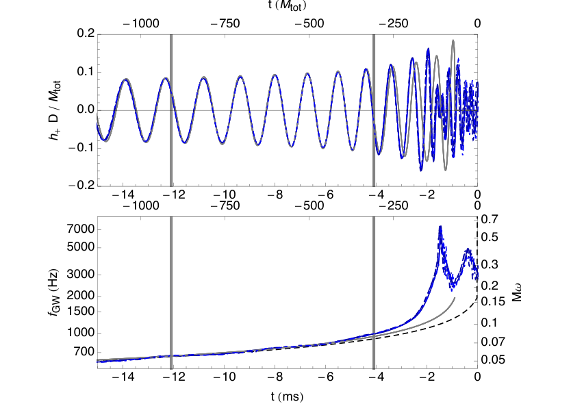

We use only the final orbits and transition to merger from the numerical waveforms, as captured in the final 10 ms or before merger: specifically, the match region is set relative to the time of peak amplitude for each numerical waveform, from ms to ms. The numerical waveform is aligned to post-Newtonian inspiral by the maximum correlation above, and then a hybrid waveform is constructed by windowing between inspiral and numerical waveforms over the last half of the match region. An example of this construction is shown in Fig. 9 for the full set of variant HB waveforms. The resulting hybrids are Fourier-transformed, and the amplitude of the difference between two waveforms is calculated directly using the inner product defined in Sec. III.2.

IV.2 Measurement using hybrid waveforms
To calculate the differences between hybrid EOS, we use a somewhat less conservative estimate than in the previous sections; to save computational time, we do not include the long low-frequency portion of the waveform in our analysis and therefore cannot minimize differences over shifts in time and phase. However, the time and phase of a high-frequency waveform that is coherent with the low-frequency inspiral are no longer free parameters. Damour et al. [15] calculate the frequency range over which each waveform parameter is determined: 90% of the total from a binary neutron star inspiral is collected from frequencies below 200 Hz. Mass parameters are determined using the waveform at even lower frequencies, and tidal effects on the inspiral are determined only by the highest-frequency portion; the two regions decouple.
We assume that the waveform portion below Hz, which is virtually identical for models of different EOS, will fix the relative time and phase of template and signal waveforms; if the overlap of very long PN-only waveforms with different tidal contributions is maximized over variations in time and phase, the relative time of coalescence is approximately that of waveforms which are exactly aligned at Hz. We then consider only differences that accumulate from Hz and up when comparing waveforms of different EOS. The resulting phase accumulation is shown in Fig. 10. With the contributions from the inspiral, the differences between the hybrid waveforms become more significant. The SNR of the differences between all pairs of waveforms is shown in Table 6. Fig. 11 illustrates the Fourier transform of the difference between pairs of waveforms, in which one member has EOS H, plotted as a signal against the Advanced LIGO noise curve.
As before, we compile the set of differences for all waveform pairs into a plot of vs. in Fig. 12. The result is again not linear in , so the statistical error estimate will depend nonlinearly on the loudness of the signal. At the reference Mpc, the difference between waveforms has for , allowing each EOS to be distinguished from a binary black hole. Marginally distinguishable parameter differences are at then at and at Mpc (where BNS inspirals are detected with and ). This means that a combination of weaker signals can be used to give significant constraints on the EOS, as seen in [95].
Advanced LIGO high-power detuned
| EOS | 2H | H | HB | B | Bss |
|---|---|---|---|---|---|
| SNR | 33.72 | 33.78 | 33.78 | 33.79 | 33.80 |
| 2H | 0.080.06 | 6.700.01 | 7.050.01 | 7.280.01 | 7.50.01 |
| H | 0.080.10 | 2.180.02 | 3.060.03 | 3.820.01 | |
| HB | 0.130.10 | 1.870.09 | 2.940.02 | ||
| B | (symm.) | 0.350.31 | 2.010.09 | ||
| Bss | 0.070.08 |
IV.3 Additional systematics with hybridization
The systematic error stemming from alternate methods of generating the waveforms and alignment used to calculate measurability can be estimated using Eq. (20) where the two waveforms and may be taken to be different hybrid waveforms. As hybrid waveforms incorporate choices in the construction beyond simply choosing the numerical waveform, additional systematic errors are introduced.
Systematic errors are estimated using the set of “well-resolved” waveforms, using the criteria of Sec. II.4, which have phase differences of radians to radians over the last ms (1100) before merger. For a fixed hybrid construction method and PN model, the diagonal entries of Table 6 give at Mpc, for of roughly 5–20% from variant numerical simulations of these EOS.
| Hybrid Variation | PN Inspiral | |||
|---|---|---|---|---|
| EOS | aLIGO | ET-D | aLIGO | ET-D |
| 2H SACRA R309 I188 | 1.60 | 14.86 | 2.34 | 22.08 |
| 2H SACRA R274 I188 | 1.48 | 13.73 | 2.34 | 22.13 |
| 2H SACRA R247 I188 | 1.46 | 13.52 | 2.35 | 22.22 |
| 2H Whisky R177 I188 | 1.16 | 10.63 | 2.34 | 22.09 |
| 2H Whisky R142 I188 | 1.08 | 09.90 | 2.35 | 22.22 |
| H SACRA R209 I221 | 0.97 | 08.57 | 1.75 | 15.71 |
| H SACRA R188 I221 | 0.87 | 07.66 | 1.75 | 15.62 |
| HB SACRA R194 I188 | 0.88 | 07.67 | 1.68 | 14.90 |
| HB SACRA R175 I188 | 0.89 | 07.76 | 1.62 | 14.40 |
| HB Whisky R177 I188 | 1.09 | 09.53 | 1.65 | 14.63 |
| HB Whisky R177 I221 | 0.93 | 08.15 | 1.63 | 14.44 |
| B SACRA R174 I221 | 0.90 | 07.79 | 1.58 | 13.87 |
| B SACRA R156 I221 | 0.85 | 07.41 | 1.42 | 12.48 |
| B Whisky R177 I221 | 1.32 | 11.53 | 1.62 | 14.26 |
| Bss SACRA R127 I221 | 1.36 | 11.80 | 1.48 | 12.88 |
| Bss Whisky R142 I221 | 1.47 | 12.83 | 1.48 | 12.90 |
We explore the impact of changing hybridization procedures by shifting the window used to match PN and numerical waveforms, within the assumptions outlined in Sec. IV.1. The procedure of Sec. IV.2 is repeated with a variant match window of ms to ms. The results for , distinguishability, and measurability of do not change appreciably. However, the systematic error from differences between numerical simulations doubles as earlier inspiral portions of lower-resolution numerical waveforms come into play.
We estimate the impact of uncertainty in the hybridization procedure used to produce parameter-estimation templates by comparing waveforms constructed from the same numerical simulation using different hybridization windows. The results in Table 7 show that the variant hybridization gives –, which decreases with increasing resolution. Even with the best resolution, ranges from 20–75% of at 100 Mpc, largest for compact stars and small differences in EOS. As in the binary black hole case [82], longer and more accurate numerical simulations will be required to reduce the systematic error associated with hybridization. We also note that while these variants seem to cover a reasonable range given the assumptions outlined in Sec. IV.1, a more systematic analysis with accurate waveforms would be required to quantify the uncertainties for parameter estimation.
The tidal contributions discussed in this paper include the leading order and next-to-leading order tidal contributions from [96, 97]. The significance of higher-order PN tidal terms can be estimated by dropping the next-to-leading order tidal contribution. This results in systematic error of – of at 100 Mpc; always smaller than systematic error from varying the hybrid procedure, but most important for large-radius stars.
We have throughout assumed that an underlying point-particle inspiral model is accurate up to . In practice, for equal-mass systems, the time-domain Taylor-T4 signal appears to satisfy this requirement, but calibrated phenomenological or EOB models may be required to accurately capture the underlying dynamics of more general systems. We also assume, based on the agreement seen in [19, 20], that there are no EOS effects beyond tidal contributions before the hybridization times used in this paper; this neglects any contributions smaller than best current numerical errors and low-frequency resonances [98].
V Use of inspiral-only templates
We can also estimate the impact of neglecting numerical simulation results entirely in a waveform model of binary neutron star inspiral and merger. To do this, we calculate the difference between the hybrid waveforms and our inspiral model extended to coalescence. The total is shown in Table 7. For compact stars (EOS B, Bss), the hybrid error is comparable to the error from neglecting the numerical merger entirely. However, larger neutron stars (EOS 2H, H) have a reduction in systematic error from using hybrids instead of inspiral-only waveforms.
One can estimate the extent to which inspiral-only waveforms can be trusted by considering an inner product calculated only up to an upper cutoff frequency. The frequency dependence of the difference between hybrid and inspiral-only waveforms is shown in Fig. 13. If this cutoff frequency is low, or the signal is weak, there is no measurable impact from using inspiral-only waveforms. All hybrids and analytic inspirals agree (to within numerical error) below 700 Hz. However, strong signals or large neutron stars produce significant differences from post-Newtonian models. The EOS 2H model, which is an extremely large ( km) neutron star, begins to depart from post-Newtonian inspiral at approximately 700 Hz, even if the hybrid window includes higher frequencies, and hybrids constructed for EOS 2H reach (distinguishable at with total ) at Hz. Hybrids for more realistic EOS (H and HB) are not distinguishable from post-Newtonian inspiral until total SNR and upper frequency Hz to Hz, although this is sensitive to the choice of hybridization window.
Aside from the systematic error introduced by using inspiral-only waveforms to measure EOS effects, one can consider the usefulness of inspiral-only models to estimate EOS measurability. In Fig. 12, we overlay the result of an analogous estimation using only post-Newtonian inspirals, including leading order and next-to-leading order tidal effects, and extended to post-Newtonian coalescence. We again again align waveforms at 200 Hz and use only differences above 200 Hz in the calculation, and also consider the same finite parameter spacings. For small differences in EOS, the PN inspiral models accurately mimic the measurability estimates of hybrid EOS. The nonlinear behavior is also seen, but for large EOS differences there is some overestimate from using inspiral-only models; this could be improved by using post-Newtonian inspirals cut-off at a representative merger frequency.
VI Multiple Signals
A combination of identical signals, each with uncertainty would give an overall uncertainty if all events occurred at the same effective distance . When scales linearly with , we can use the results of [99] to estimate how the uncertainty at a reference translates to an expected combined error from signals randomly distributed within a horizon distance . The combined uncertainty from the signals is given by
| (24) |
where is the total number of events.
For the numerical-only estimates, linear scaling does not apply. We take the maximum range where we have calculated distinguishability of signals, at Mpc, within which we expect to find equalling 9% of the total number of signals (again following [10]). We conservatively take linear scaling from this limiting distinguishability, and find .
For hybrid estimates, we can use the dotted line in Fig. 12, which gives for Mpc, to provide a roughly linear scaling within the horizon distance of 445 Mpc. Eq. (24) then gives an estimate for the expected measurement uncertainty of .
We expect, from studies with mixed binaries [88], that correlations with mass parameters will increase by a factor of . Full bayesian parameter estimation using post-Newtonian waveforms including tidal terms suggests that a combination of multiple signals can still used to distinguish between realistic EOS[95]. However, the statistical uncertainty would then be significantly smaller than the systematic errors estimated in this work, which do not decrease with number of signals. Uncertainty in waveform modeling would therefore limit our ability to measure EOS parameters using binary neutron star systems.
VII Conclusions
It is now clear that tidal effects due to the finite size of neutron stars can produce a detectable signature in gravitational signals that are likely to be observed by ground-based gravitational wave detectors such as Advanced LIGO. The observation of these tidal effects presents the possibility of measuring neutron star properties which in turn will constrain models for the neutron-star EOS. In particular, using only numerical simulations of the final orbits, we estimate two EOS, H and B, which produce isolated neutron-star radii that differ by , are distinguishable at Mpc. This gives an effective %. However, the measurement accuracy does not improve linearly with SNR, and weaker signals will have less discriminatory power.
If trusted hybrids can be constructed, incorporating additional information from the tidal post-Newtonian terms, then measurement errors drop significantly, and the above EOS can be distinguished at Mpc. Numerical relativity efforts are required to generate the waveforms needed to make these measurements, but the current state-of-the-art simulations are already up to the task for large-radius neutron stars. Future advances in numerical relativity will provide waveforms of higher accuracy, and extending to lower frequencies, which will reduce systematic errors on measurements of tidal effects. Further improvements in the scope of physical processes that are simulated by numerical relativity will also enable us to follow the waveform through binary coalescence and past merger, and therefore could allow for the measurement of additional EOS properties from oscillations of a post-merger hypermassive remnant.
Acknowledgements.
This work was supported by Grant-in-Aid for Scientific Research (24740163) of Japanese MEXT, by NSF awards PHY-1055103, PHY-0970074, PHY-0900735, PHY-0701817, PHY-0503366, and PHY-1001515, and by the Grant-in-Aid for Young Scientists (22740163). B.G. acknowledges support from NSF grant no. AST 1009396 and NASA Grant No. NNX12AO67G. This work used XSEDE (allocation TG-PHY110027) which is supported by NSF Grant No. OCI-1053575. K.K. is supported by JSPS Postdoctoral Fellowship for Research Abroad. CM acknowledges support by NSF Grant PHY1001515, DFG grant SFB/Transregio 7 “Gravitational Wave Astronomy” and STFC grant PP/E001025/1. We thank B. D. Lackey for reading a draft of the paper and suggesting changes, for helpful conversations, and for providing Fig. 2. J.S.R. thanks the the “Rattle and Shine” workshop at KITP (Santa Barbara) and the “YKIS2013” workshop at YITP (Kyoto) for useful discussions.References
- [1] A. W. Steiner, J. M. Lattimer, and E. F. Brown, The Astrophysical Journal 722, 33 (2010).
- [2] T. Guver, D. Psaltis, and F. Ozel, ArXiv e-prints (2011), arXiv:1103.5767 [astro-ph.HE] .
- [3] F. Özel and D. Psaltis, Phys. Rev. D 80, 103003 (2009), arXiv:0905.1959 [astro-ph.HE] .
- [4] F. Özel, D. Psaltis, S. Ransom, P. Demorest, and M. Alford, Astrophys. J. Lett. 724, L199 (2010a), arXiv:1010.5790 [astro-ph.HE] .
- [5] F. Özel, G. Baym, and T. Güver, Phys. Rev. D 82, 101301 (2010b), arXiv:1002.3153 [astro-ph.HE] .
- [6] V. Suleimanov, J. Poutanen, M. Revnivtsev, and K. Werner, ArXiv e-prints (2010), arXiv:1004.4871 [astro-ph.HE] .
- [7] M. Zamfir, A. Cumming, and D. K. Galloway, The Astrophysical Journal 749, 69 (2012), arXiv:1111.0347 [astro-ph.SR] .
- [8] C. Cutler and E. E. Flanagan, Phys. Rev. D 49, 2658 (1994).
- [9] G. M. Harry and the LIGO Scientific Collaboration, Classical and Quantum Gravity 27, 084006 (2010).
- [10] J. Abadie et al. (LIGO Scientific), Class. Quant. Grav. 27, 173001 (2010), arXiv:1003.2480 [Unknown] .
- [11] E. Flanagan and T. Hinderer, Physical Review D 77 (2008), 10.1103/PhysRevD.77.021502.
- [12] T. Damour and A. Nagar, Physical Review D 81, 21 (2010).
- [13] J. Vines, E. E. Flanagan, and T. Hinderer, Phys. Rev. D83, 084051 (2011), arXiv:1101.1673 [gr-qc] .
- [14] T. Hinderer, B. Lackey, R. Lang, and J. S. Read, Physical Review D 81, 1 (2010).
- [15] T. Damour, A. Nagar, and L. Villain, Phys. Rev. D 85, 123007 (2012), arXiv:1203.4352 [gr-qc] .
- [16] J. Read, B. Lackey, B. Owen, and J. Friedman, Physical Review D 79, 124032 (2009a).
- [17] L. Baiotti, T. Damour, B. Giacomazzo, A. Nagar, and L, Physical Review Letters 105, 261101 (2010a).
- [18] L. Baiotti, T. Damour, B. Giacomazzo, A. Nagar, and L. Rezzolla, Physical Review D 84, 1 (2011).
- [19] S. Bernuzzi, A. Nagar, M. Thierfelder, and B. Brügmann, (2012), arXiv:1205.3403 [gr-qc] .
- [20] K. Hotokezaka, K. Kyutoku, and M. Shibata, Phys. Rev. D 87, 044001 (2013), arXiv:1301.3555 [gr-qc] .
- [21] M. Shibata, Physical Review Letters 94, 4 (2005).
- [22] A. Bauswein, H.-T. Janka, and R. Oechslin, Arxiv preprint , 10 (2010).
- [23] N. Stergioulas, A. Bauswein, K. Zagkouris, and H.-T. Janka, MNRAS 418, 427 (2011), arXiv:1105.0368 [gr-qc] .
- [24] T. Yamamoto, M. Shibata, and K. Taniguchi, Physical Review D 78 (2008), 10.1103/PhysRevD.78.064054.
- [25] L. Baiotti, I. Hawke, P. Montero, and L. Rezzolla, in Computational Astrophysics in Italy: Methods and Tools, Vol. 1, edited by R. Capuzzo-Dolcetta (MSAIt, Trieste, 2003) p. 210.
- [26] L. Baiotti, I. Hawke, P. J. Montero, F. Löffler, L. Rezzolla, N. Stergioulas, J. A. Font, and E. Seidel, Phys. Rev. D 71, 024035 (2005).
- [27] B. Giacomazzo and L. Rezzolla, Class. Quantum Grav. 24, S235 (2007), gr-qc/0701109 .
- [28] J. S. Read, C. Markakis, M. Shibata, K. Uryū, J. D. E. Creighton, and J. Friedman, Physical Review D 79, 1 (2009b).
- [29] K. Kyutoku, M. Shibata, and K. Taniguchi, Phys. Rev. D 82, 044049 (2010), arXiv:1008.1460 [astro-ph.HE] .
- [30] K. Hebeler, J. Lattimer, C. Pethick, and A. Schwenk, Physical Review Letters 105, 161102 (2010).
- [31] P. B. Demorest, T. Pennucci, S. M. Ransom, M. S. E. Roberts, and J. W. T. Hessels, Nature (London) 467, 1081 (2010), arXiv:1010.5788 [astro-ph.HE] .
- [32] K. Taniguchi and M. Shibata, Astrophys. J. Suppl. 188, 187 (2010), arXiv:1005.0958 [astro-ph.SR] .
- [33] D. Pollney, C. Reisswig, L. Rezzolla, B. Szilágyi, M. Ansorg, B. Deris, P. Diener, E. N. Dorband, M. Koppitz, A. Nagar, and E. Schnetter, Phys. Rev. D 76, 124002 (2007).
- [34] L. Baiotti, B. Giacomazzo, and L. Rezzolla, Phys. Rev. D 78, 084033 (2008), arXiv:0804.0594 [gr-qc] .
- [35] E. Gourgoulhon, P. Grandclément, K. Taniguchi, J. A. Marck, and S. Bonazzola, Phys. Rev. D 63, 064029 (2001).
- [36] K. Taniguchi and E. Gourgoulhon, Phys. Rev. D 66, 104019 (2002).
- [37] K. Taniguchi and E. Gourgoulhon, Phys. Rev. D 68, 124025 (2003).
- [38] http://www.lorene.obspm.fr.
- [39] T. Nakamura, K. Oohara, and Y. Kojima, Prog. Theor. Phys. Suppl. 90, 1 (1987).
- [40] M. Shibata and T. Nakamura, Phys. Rev. D 52, 5428 (1995).
- [41] T. W. Baumgarte and S. L. Shapiro, Phys. Rev. D 59, 024007 (1998), gr-qc/9810065 .
- [42] M. Alcubierre, B. Brügmann, T. Dramlitsch, J. A. Font, P. Papadopoulos, E. Seidel, N. Stergioulas, and R. Takahashi, Phys. Rev. D 62, 044034 (2000), gr-qc/0003071 .
- [43] T. Goodale, G. Allen, G. Lanfermann, J. Massó, T. Radke, E. Seidel, and J. Shalf, in Vector and Parallel Processing – VECPAR’2002, 5th International Conference, Lecture Notes in Computer Science (Springer, Berlin, 2003).
- [44] C. W. Misner, K. S. Thorne, and J. A. Wheeler, Gravitation, Misner73 (W. H. Freeman, San Francisco, 1973).
- [45] C. Bona, J. Massó, E. Seidel, and J. Stela, Phys. Rev. Lett. 75, 600 (1995), gr-qc/9412071 .
- [46] M. Alcubierre, B. Brügmann, P. Diener, M. Koppitz, D. Pollney, E. Seidel, and R. Takahashi, Phys. Rev. D 67, 084023 (2003), gr-qc/0206072 .
- [47] J. M. Martí, J. M. Ibáñez, and J. A. Miralles, Phys. Rev. D 43, 3794 (1991).
- [48] F. Banyuls, J. A. Font, J. M. Ibáñez, J. M. Martí, and J. A. Miralles, Astrophys. J. 476, 221 (1997).
- [49] J. Ibáñez, M. Aloy, J. Font, J. Martí, J. Miralles, and J. Pons, in Godunov methods: theory and applications, edited by E. Toro (Kluwer Academic/Plenum Publishers, New York, 2001).
- [50] J. A. Font, Living Rev. Relativ. 6, 4 (2003).
- [51] P. Colella and P. R. Woodward, J. Comput. Phys. 54, 174 (1984).
- [52] A. Kurganov and E. Tadmor., J. Comput. Phys. 160, 241 (2000).
- [53] M. A. Aloy, J. M. Ibáñez, J. M. Martí, and E. Müller, Astrophys. J. Suppl. 122, 151 (1999).
- [54] L. Baiotti, M. Shibata, and T. Yamamoto, Physical Review D 82, 1 (2010b).
- [55] E. Schnetter, S. H. Hawley, and I. Hawke, Class. Quantum Grav. 21, 1465 (2004).
- [56] E. T. Newman and R. Penrose, J. Math. Phys. 3, 566 (1962), erratum in J. Math. Phys. 4, 998 (1963).
- [57] L. Gunnarsen, H. Shinkai, and K. Maeda, Class. Quantum Grav. 12, 133 (1995), gr-qc/9406003 .
- [58] S. A. Teukolsky, Astrophys. J. 185, 635 (1973).
- [59] L. Baiotti, S. Bernuzzi, G. Corvino, R. De Pietri, and A. Nagar, Phys. Rev. D 79, 024002 (2009), arXiv:0808.4002 [gr-qc] .
- [60] C. Reisswig and P. D., Calss. Quantum Grav. 28, 195015 (2011), arXiv:1006.1632 [gr-qc] .
- [61] K. Kyutoku, H. Okawa, M. Shibata, and K. Taniguchi, Phys. Rev. D 84, 064018 (2011), arXiv:1108.1189 [astro-ph] .
- [62] V. Moncrief, Annals of Physics 88, 323 (1974).
- [63] M. Hannam, S. Husa, J. Baker, M. Boyle, B. Brügmann, T. Chu, N. Dorband, F. Herrmann, I. Hinder, B. Kelly, L. Kidder, P. Laguna, K. Matthews, J. van Meter, H. Pfeiffer, D. Pollney, C. Reisswig, M. Scheel, and D. Shoemaker, Physical Review D 79, 084025 (2009).
- [64] M. Shibata, K. Taniguchi, and K. Uryū, Phys. Rev. D 68, 084020 (2003), arXiv:gr-qc/0310030 .
- [65] M. Shibata, K. Taniguchi, and K. Uryū, Phys. Rev. D 71, 084021 (2005), arXiv:gr-qc/0503119 .
- [66] M. Shibata and K. Taniguchi, Phys. Rev. D 73, 064027 (2006), arXiv:astro-ph/0603145 .
- [67] R. Oechslin and H.-T. Janka, Phys. Rev. Lett. 99, 121102 (2007).
- [68] K. Hotokezaka, K. Kyutoku, H. Okawa, M. Shibata, and K. Kiuchi, Phys. Rev. D 83, 124008 (2011), arXiv:1105.4370 [astro-ph.HE] .
- [69] K. Yagi and N. Yunes, ArXiv e-prints (2013), arXiv:1302.4499 [gr-qc] .
- [70] Y. Sekiguchi, K. Kiuchi, K. Kyutoku, and M. Shibata, Phys. Rev. Lett. 107, 051102 (2011), arXiv:1105.2125 [gr-qc] .
- [71] L. Rezzolla, L. Baiotti, B. Giacomazzo, D. Link, and J. A. Font, Classical Quantum Gravity 27, 114105 (2010), arXiv:1001.3074 [gr-qc] .
- [72] D. Shoemaker, Advanced LIGO anticipated sensitivity curves, Tech. Rep. LIGO-T0900288-v2 (LIGO, 2009) the high-power detuned model used in this paper is given in the data file ZERO_DET_high_P.txt.
- [73] S. Hild et al., Class. Quant. Grav. 28, 094013 (2011), arXiv:1012.0908 [gr-qc] .
- [74] L. Santamaría, F. Ohme, P. Ajith, B. Brügmann, N. Dorband, M. Hannam, S. Husa, P. Mösta, D. Pollney, C. Reisswig, E. Robinson, J. Seiler, and B. Krishnan, Physical Review D 82, 22 (2010).
- [75] B. Iyer, T. Souradeep, C. Unnikrishnan, S. Dhurandhar, S. Raja, and A. Sengupta, LIGO-India, Proposal of the Consortium for Indian Initiative in Gravitational-wave Observations (IndIGO), Tech. Rep. LIGO-M1100296-v2 (LIGO, 2012).
- [76] T. V. Collaboration, Advanced Virgo Baseline Design, Tech. Rep. VIR-0027A-09 (2009).
- [77] K. Somiya, Classical and Quantum Gravity 29, 124007 (2012), arXiv:1111.7185 [gr-qc] .
- [78] A. Bauswein, H.-T. Janka, K. Hebeler, and A. Schwenk, ArXiv e-prints (2012), arXiv:1204.1888 [astro-ph.SR] .
- [79] J. D. E. Creighton, Phys. Rev. D 60, 022001 (1999).
- [80] S. Fairhurst, Result presented at the “Interplay between Numerical Relativity and Data Analysis” workshop at the KITP, UCSB, January 2008.
- [81] L. Lindblom, B. J. Owen, and D. A. Brown, Phys. Rev. D78, 124020 (2008), arXiv:0809.3844 [gr-qc] .
- [82] I. MacDonald, S. Nissanke, and H. P. Pfeiffer, Classical and Quantum Gravity 28, 134002 (2011).
- [83] B. Allen, W. G. Anderson, P. R. Brady, D. A. Brown, and J. D. E. Creighton, ArXiv e-prints (2005), arXiv:gr-qc/0509116 .
- [84] H.-S. Cho, E. Ochsner, R. O’Shaughnessy, C. Kim, and C.-H. Lee, Phys. Rev. D 87, 024004 (2013).
- [85] C. Cutler and M. Vallisneri, Phys. Rev. D 76, 104018 (2007).
- [86] L. S. Finn, Phys. Rev. D46, 5236 (1992), arXiv:gr-qc/9209010 .
- [87] B. D. Lackey, K. Kyutoku, M. Shibata, P. R. Brady, and J. L. Friedman, Phys. Rev. D 85, 044061 (2012), arXiv:1109.3402 [astro-ph.HE] .
- [88] B. D. Lackey, K. Kyutoku, M. Shibata, P. R. Brady, and J. L. Friedman, ArXiv e-prints (2013), arXiv:1303.6298 [gr-qc] .
- [89] M. Hannam, S. Husa, F. Ohme, and P. Ajith, Arxiv preprint , 1 (2010).
- [90] S. Bernuzzi, M. Thierfelder, and B. Brügmann, Arxiv preprint (2011), arXiv:1109.3611 .
- [91] M. Boyle, D. A. Brown, L. E. Kidder, A. H. Mroué, H. P. Pfeiffer, M. A. Scheel, G. B. Cook, and S. A. Teukolsky, Phys. Rev. D 76, 124038 (2007), arXiv:0710.0158 [gr-qc] .
- [92] T. Damour, B. R. Iyer, and B. S. Sathyaprakash, Phys. Rev. D 63, 044023 (2001), arXiv:gr-qc/0010009 .
- [93] K. D. Kokkotas and G. Schaefer, Monthly Notices of the Royal Astronomical Society 275, 301 (1995).
- [94] M. Boyle, D. A. Brown, and L. Pekowsky, Classical and Quantum Gravity 26, 114006 (2009).
- [95] W. del Pozzo, T. G. F. Li, M. Agathos, C. van den Broeck, and S. Vitale, in prep .
- [96] J. Vines and É. É. Flanagan, ArXiv e-prints (2010), arXiv:1009.4919 [gr-qc] .
- [97] J. Vines, T. Hinderer, and É. É. Flanagan, ArXiv e-prints (2011), arXiv:1101.1673 [gr-qc] .
- [98] P. Balachandran and E. Flanagan, Arxiv preprint , 3 (2007).
- [99] C. Markakis, J. S. Read, M. Shibata, K. Uryu, J. D. E. Creighton, and J. L. Friedman, ArXiv e-prints (2010), arXiv:1008.1822 [gr-qc] .