Anisotropic imprint of long-wavelength tensor perturbations on cosmic structure
Abstract
Inflationary models predict a correlation between primordial density perturbations (scalar metric perturbations) and gravitational waves (tensor metric perturbations) in the form of a scalar-scalar-tensor three-point correlation, or bispectrum in Fourier space. The squeezed limit of this bispectrum implies a quadrupolar asymmetry in the observed local power spectrum for matter and galaxies. Here we show (like others before) that an infrared divergence in the amplitude of this power asymmetry predicted in single-field slow-roll models is canceled by projection effects when considering the observed power spectrum. We then further evaluate the nonzero, but finite, residual quadrupolar power asymmetry that remains after the divergences are canceled. While the quadrupolar power asymmetry is small, it is conceptually important. Our calculation moreover clarifies how the predictions for this power asymmetry may change in models with different scalar-scalar-tensor bispectra, and shows that convincing detection of the quadrupolar power asymmetry would rule out the single-field slow-roll models of inflation.
I Introduction
Three decades of increasingly precise measurements, culminating most recently with those from the Planck satellite [1], have all shown consistency with the simplest single-field slow-roll (SFSR) models of inflation [2, 3, 4, 5, 6]. Still, many questions about the new physics responsible for inflation remain, and a number of further predictions of inflation remain to be tested. One of these predictions is a stochastic background of gravitational waves, or tensor metric perturbations [7, 8, 9, 10]. Efforts are now underway to detect these tensor modes in the cosmic microwave background (CMB) polarization [11, 12], and there are prospects for direct detection of the background [13, 14, 15, 16].
There may, however, also be an imprint of tensor modes in the observed cosmic mass distribution. One possible observable is the distortion induced by gravitational lensing by tensor modes to the galaxy distribution [17, 18, 19], the CMB [20, 21, 22, 23] or the 21-cm background [24, 25, 26]. Another possibility—which we focus upon here—is that long-wavelength tensor perturbations may lead to a quadrupolar power asymmetry in the power spectra for scalar perturbations. The idea is simple: tensor modes with wavelengths longer than the distance over which observations are done give rise to a quadrupolar distortion to the spacetime over the observed volume. This quadrupole may then (a) get imprinted somehow in the primordial mass distribution and/or (b) induce a quadrupole in the observed distribution through projection effects. Such a quadrupole could then be sought, for example, in the cosmic microwave background [27, 28] or in galaxy surveys [29]. In fact, null searches for power asymmetries have already been carried out in galaxy surveys [30]. A tentative detection in the CMB [31] was later disputed; current measurements place upper limits [32, 33] at the level of on the amplitude of a power quadrupole.
One might think that the amplitude of the power asymmetry would be large. For example, in standard SFSR inflation, the contribution to the square of the local tensor-perturbation amplitude is equal across each logarithmic interval of tensor wavelength. The root-mean-square (rms) of the local quadrupolar distortion then scales with total number of -folds of inflation, and this number could conceivably be large. An explicit calculation of the scalar-scalar-tensor power quadrupole [34, 35], based upon the SFSR scalar-scalar-tensor bispectrum [36], seems to show such an infrared divergence. An upper limit on the power asymmetry would then translate into an upper bound to the duration of inflation. Roughly speaking, the power quadrupole obtained this way is ,11 1 We use instead of for tensor modes. where is the number of -folds, and is the typical amplitude for a given Fourier mode of the tensor field in terms of the energy density during inflation and the Planck mass . A conservative current upper limit of for the power quadrupole [30, 32, 33] then translates to .
On second thought, there are several reasons to question this result. First of all, it seems strange that observables within our horizon (which is contained within the last -folds of inflation) could be probing physics on scales many orders of magnitude beyond the observable horizon. This becomes even clearer when we realize that as the tensor wavenumber , a given Fourier mode of the tensor field approaches a constant tensor perturbation to the metric. However, the coordinates in a metric with a constant tensor can always be re-scaled to give a Friedman-Robertson-Walker metric. In other words, observables only depend on (at least two) spacetime derivatives, , of the tensor metric perturbation . True, a perturbation of arbitrarily long wavelength was presumably within the horizon at some sufficiently early time during inflation. But again, it seems strange that observables within our horizon would depend on asymptotically early times during inflation. These arguments thus suggest that the infrared divergence in the power quadrupole is a gauge artifact.
Since Maldacena’s paper [36] on three-point functions in inflation, a large literature (e.g., Refs. [37, 38, 39, 40, 41, 42]) has clarified that analogous divergences that arise from the squeezed limit of the scalar-scalar-scalar bispectrum are gauge artifacts. Refs. [36, 37] point out that the only effect of the squeezed-limit bispectrum in terms of the global synchronous-gauge coordinates used in Ref. [36] is a constant coordinate transform into the local Fermi normal coordinates (FNC). Ref. [39] splits perturbations into small- and long-wavelength modes and absorbs the latter into the background. Ref. [40] defines genuine gauge-invariant variables, whose bispectrum explicitly vanishes in the squeezed limit. While there are some differences (to be expanded upon below), many of those arguments apply to the squeezed limit of the scalar-scalar-tensor bispectrum. As clarified most recently in Ref. [43], and also below, the divergence in the primordial power quadrupole from the scalar-scalar-tensor bispectrum is canceled precisely by projection effects induced by the tensor perturbation at late times.
We show here, however, that there still remains in SFSR inflation, after these divergences cancel, a nonzero but finite quadrupolar asymmetry in the observed local power spectrum. Here local means that the power spectrum is measured within a patch smaller than the wavelength of the tensor mode.22 2 The quadrupolar asymmetry in the three-dimensional power spectrum we focus on here should not be confused with the quadrupolar component () of some two-dimensional angular power spectrum . While the switch, employed in previous work [43], to FNC coordinates right after inflation suffices to demonstrate the cancellation of divergences, it fails to account for the effects of spatial and temporal variations of tensor perturbations [44]. Both FNC and the peak-background split are only valid locally and hence introduce ambiguities for finite Fourier wavelengths. In this paper we therefore work with global FRW coordinates but define observables in a physical way. For simplicity, we first derive rigorous results for a post-inflation Universe filled with non-relativistic matter. We then argue heuristically, but without a complete calculation, that the power quadrupole induced by tensor modes of the smaller wavelengths that enter the horizon during radiation domination should be suppressed. The calculation presented here thus applies to tensor modes outside the horizon and to modes within the horizon today but that entered the horizon during matter domination (i.e., with wavelengths ). This allows us to account for the epoch of radiation domination that precedes matter domination. Dark energy dominates only at very late times and thus plays a marginal role on the power quadrupole. It does affect the mapping between source redshift and comoving distance though. With these insights, we are able to generalize our results and make contact with our Universe. Our work expands upon previous work [44], which also suggested a finite effect on the observed power spectrum that grows logarithmically with time, by making precise the prediction for observable quantities.
Our calculation shows that the observable power asymmetry depends on spacetime derivatives of the tensor perturbation, rather than just its amplitude. As a result, the contribution from a given superhorizon mode to the observable power asymmetry is suppressed by a factor relative to the naive calculation. Thus, local observables are not sensitive to inflationary tensor modes with arbitrarily long wavelength. Our conclusion is based on three considerations: (1) the squeezed primordial scalar-scalar-tensor bispectrum satisfies the single-field consistency relation [Eq. (3) below]; (2) throughout the expansion history after inflation, nonlinear mode couplings between long-wavelength tensor perturbations and short-wavelength scalar perturbations take effect; (3) the positions at which we correlate matter/galaxy overdensities are specified in a physical way, e.g. by the observed redshifts and the observed angular position on the sky.
We then find that the observable power quadrupole is induced at any given time predominantly by tensor perturbations with wavelengths comparable to the horizon at that time, as it should be. While the amplitude (rather than ) of the resulting quadrupolar power asymmetry is too small to be observable today, it is important conceptually to note that the power asymmetry exists. We also note that in models where the self-consistency relation is violated [45],33 3 Also for violations of the scalar-scalar-scalar consistency relation, see, e.g., Ref. [42, 46] the power quadrupole could conceivably be far larger. A null detection can thus constrain such alternative models. Conversely, detection of a power quadrupole would rule out SFSR inflation.
We begin in Sec. II with a discussion of our notations. We then review in Sec. III the primordial scalar-scalar-tensor correlation. Sec. IV considers the evolution of scalar perturbations in the presence of a tensor perturbation. Sec. V then connects the results of the previous Section to the observed galaxy distribution, determined from redshifts and angular positions of galaxies. Sec. VI comments on the generalization of the calculation beyond the purely matter-dominated case, and Sec. VII then evaluates numerically the amplitude of the quadrupolar power asymmetry. Sec. VIII makes concluding remarks. Many of the calculational details are presented in the Appendixes. Appendix A derives the two-point correlation function for scalar perturbations in the presence of a tensor mode. Appendix B presents some details for the derivation of the Einstein and fluid equations in the Poisson gauge. Appendix C solves equations for the nonlinear evolution of density perturbations in the presence of a tensor perturbation. Appendix D presents an alternative derivation of the central result, Eq. (14), by tracking with Lagrangian coordinates a collection of freely-falling test particles. Appendix E provides the mapping between galaxy overdensities in general coordinates and observed coordinates, and Appendix F derives the galaxy power spectrum in observed coordinates. Finally, Appendix G collects useful results for calculating the power quadrupole.
II Notation
At the end of inflation, all perturbations of interest extend well beyond the horizon. They are conveniently described in a global comoving coordinate system, which allows for perturbative calculations across all scales. We choose the Poisson gauge [47], in which the perturbed Friedmann-Robertson-Walker (FRW) metric reads,
| (1) | |||||
Here Latin indices are for three-dimensional flat space, and they are raised and lowered by Kronecker deltas and . The two potentials and encode scalar perturbations, while the traceless, divergence-free encodes tensor perturbations. We have chosen to factor out instead of writing . This ensures that for tensor perturbations with infinite wavelength—i.e. a constant —the only effect is a trivial rescaling of spatial coordinates . The time-space components of the metric perturbations are divergence-free . In the absence of primordial vector perturbations, only appears at second order [48], and does not affect the result for that we obtain here; we thus neglect it hereafter.
The primordial values for metric perturbations are labeled with a subscript p. In later Sections, when we consider the projection effect, we need to consider only the (linear) tensor metric perturbations,
| (2) |
Lower-case ’s are reserved for wavevectors of scalar perturbations, and uppercase for wavevectors of tensor perturbations. An overdot denotes the derivative with respect to comoving time , not to be confused with the conformal time . For conciseness, we suppress the time dependence of variables whenever the suppression can induce no ambiguity. It is then understood that the equations hold at any given cosmic time.
Observed quantities (positions, perturbations, correlation functions, etc.) will be labeled with a tilde, as opposed to their counterparts computed in global FRW coordinates. The precise meaning of “observed” will be elucidated in the Sections to follow.
The notation will be used for correlations computed in the presence of a given tensor-perturbation realization. This is to be distinguished from correlations computed for a cosmology without tensor perturbations.
III Primordial scalar power spectrum with tensor perturbations
One way inflationary tensor perturbations can impact cosmic structure formation is by distorting the primordial scalar correlation function. Inflationary dynamics typically predict correlations between a large-scale tensor mode with wavevector and polarization , and two small-scale scalar perturbations with wavevectors and . This is represented by a primordial scalar-scalar-tensor bispectrum . In many inflation scenarios, the bispectrum satisfies the consistency relation [36, 37],
| (3) |
in the squeezed limit, up to model-specific corrections suppressed by . Here we define . The logarithmic derivative of the power spectrum is , where is the scalar spectral index. The bispectrum implies that in a given realization for of the tensor field, the correlation between two modes is [34]
| (4) |
where we have summed over the two tensor polarizations.
Fourier-transforming back to real space, we can derive a scalar correlation function between two points and , with a separation and a midpoint at . A local scalar two-point correlation, as a function of , is meaningful if the correlation scale is small compared to the typical variation scale of the tensor; i.e., , or in Fourier space. In this regime (as derived in Appendix A),
| (5) |
where and its derivatives are evaluated at the midpoint . Effectively, the primordial correlations between large-scale tensor modes and small-scale scalar modes give rise to an anisotropic primordial scalar power spectrum (cf. Eq. (6) in Ref. [44] and Eq. (4.5) in Ref. [49])
| (6) | |||||
which applies to a local volume smaller than in the vicinity of . The choice of the midpoint has the advantage that the omitted corrections are at least second-order derivatives of .
Naively, Eq. (6) suggests that superhorizon tensor modes with arbitrarily long wavelengths contribute to , and hence induce a large quadrupole in the scalar power spectrum. However, modes with lead to no observable effect. To see this, consider a constant , corresponding to a tensor mode of infinite wavelength. One realizes that the same comoving separations along different directions represent different physical separations (can be defined by the proper distance, or any other coordinate-independent measure of length), since the tensor mode acts as an anisotropic background metric. The anisotropy in the scalar two-point correlation function should be measured by correlating pairs of points along different directions but with the same physical separation. In terms of physical positions, we can derive from Eq. (5),
| (7) |
Note that in the absence of on the right-hand side, . This is to say that with constant tensor perturbations we measure a physical correlation function no different than what we would measure without. We highlight the crucial role of the consistency relation that the coefficient in Eq. (3) ensures the validity of Eq. (7).
Still, Eq. (7) receives corrections, which represent genuine physical effects, of order , from the finiteness of the tensor-mode wavelength [43]. Although our aim in this paper is to find the leading-order effect of the long-wavelength tensor modes, here we neglect terms of order , because these terms are much smaller compared to the correction that we will discuss in Section V.
Note that Eq. (6) is equivalent to the scalar-scalar-tensor bispectrum, Eq. (3), in its squeezed limit (). This equation operationally defines the role of long-wavelength tensor modes: the long-wavelength tensor mode (wavenumber ) centered at modulates the local scalar power spectrum (with wavenumber ) around the point. Throughout this paper, we will express the effect of long-wavelength tensor modes in the same manner. That is, the specific situation that we are considering is in the presence of long-wavelength tensor modes at a region centered around , and we are calculating the imprint of such tensor modes on the observed galaxy/matter power spectrum.
IV Post-inflationary evolution
Large-scale tensor perturbations can also affect structure formation through nonlinear mode coupling during post-inflation evolution.
To present our approach clearly, we first work within a simplified cosmology, in which non-relativistic matter (e.g., cold dark matter) dominates the energy density after reheating. The matter component can be described as a fluid with negligible pressure and anisotropic stress. Matter perturbations, including the fractional density perturbation and peculiar velocity , then grow from the primordial scalar perturbations. Still, we will eventually consider the radiation-dominated epoch preceding matter domination to better account for our Universe in Section VI.
We start with the perturbed metric of Eq. (1) and write down the Einstein equations and fluid equations for the metric and matter perturbations, as detailed in Appendix B.
Our strategy is to treat scalar/matter perturbations (which are small only in the linear regime) and tensor perturbations (which are always small) as independent expansion parameters in the perturbative expansion. In this spirit, we keep mixed second-order terms of the order scalar/matter perturbations multiplying the tensor perturbations, but ignore terms quadratic in scalar/matter perturbation itself or in itself. The former pertains to the usual nonlinear structure formation without tensor perturbations, which has been extensively studied in the literature [50, 51]. The latter, being practically negligible, is beyond the scope of this work.
We then decompose perturbations into a linear solution (labeled (1)) plus a second-order correction (labeled (2)), e.g. , and the same for , , , and so on. For the peculiar velocity, we decompose . Here, and are the linear and second-order curl-free velocity fields, respectively, and is the divergence-free velocity field, which arises only in second order.
The linear solutions are routinely solved in the standard linear cosmological perturbation theory. The second-order corrections arise from nonlinear mode-coupling between the tensor-perturbation modes and the scalar/matter-perturbation modes.
We are not interested in the nonlinear correction for tensors, which describes gravitational-wave emission from cosmic structures. Indeed, it does not source second-order scalar/matter perturbations. Therefore, we cause no confusion by using in place of .
IV.1 Linear evolution
The linear evolution of matter perturbations during the matter-dominated epoch is easily solved.
At linear order, the peculiar velocity is curl-free. In the absence of anisotropic stress, the two scalar potentials are related via , and satisfies the differential equation . Neglecting the decaying solution, the potential is conserved, , throughout matter domination. Adiabatic initial conditions then lead to linear growth for the matter perturbations (in Fourier space),
| (8) |
where the linear-extrapolation factor for matter is .
At first order, evolves independently,
| (9) |
The solution (in Fourier space) is given by with the linear-extrapolation factor for tensor modes. The tensor amplitude is conserved outside the horizon and then oscillates and decays after horizon re-entry.
IV.2 Nonlinear tensor-scalar mode coupling
In general, the nonlinear corrections for scalar/matter perturbations satisfy the same linear, second-order differential equations as the linear solutions do, but with inhomogeneous source terms quadratic in linear solutions. They vanish at early times when perturbations are linear.
In particular, the nonlinear correction to the potential , as derived in Appendix C, can be solved from
where is given by
| (11) |
We now assume a scale hierarchy between the tensor perturbations and the scalar/matter perturbations of interest—the typical variation scale of tensors is much larger than the scale of scalar/matter perturbations; i.e., . In this regime, the variation of is unimportant compared to that of , and we can apply the inverse Laplacian only on the potential,
| (12) |
Then according to Eq. (11), the second term on the right-hand side of Eq. (IV.2) is , and hence is smaller than the first term. Like in the discussion of primordial scalar power spectrum in Sec.III, we consistently ignore this term. The solution to Eq. (IV.2) can then be obtained via a Green’s function approach,
| (13) | |||||
Then , obtained from Eq. (59), can be combined with to give the full nonlinear matter overdensity . We work in Fourier space (consider a single tensor mode with wavevector that constitutes a realization for the tensor perturbation) and insert the various results for linear solutions. A final compact expression,
| (14) | |||||
can be derived, where is understood as the primordial tensor perturbation evaluated on a comoving patch smaller than , over which small-scale matter-perturbation modes are measured. In deriving this result, we have ignored general-relativistic corrections that are suppressed by either or at observing time (see Appendix C). As a check, we present in Appendix D an alternative derivation of Eq. (14) using Lagrangian coordinates for collisionless matter in the subhorizon limit . The function (plotted in Fig. 1) is given by
| (15) |
which has asymptotic behaviors,
| (16) |
Note that corresponds exactly to the comoving horizon scale . Therefore, anisotropic matter clustering builds up only around the time of horizon re-entry of a given tensor mode. Long before re-entry, the mode is superhorizon and its influence on sub-horizon physics can be gauged away; long after re-entry, on the other hand, the tensor amplitude redshifts away and can no longer play a role.

Eq. (14) demonstrates that due to large-scale tensor perturbations, matter undergoes anisotropic clustering locally, and in Fourier space overdensity modes grow with a quadrupolar dependence on the direction of the wavevector .
IV.3 Infinite wavelength tensor
We now examine the case of a constant tensor perturbation to make the point that the nonlinear corrections from mode coupling between tensor modes and scalar/matter modes are indispensable to ensure a gauge-invariant answer for an observable such as the correlation function.
For constant , we have and . For any observation at finite , vanishes as . The matter overdensity up to nonlinear order is simply
| (17) |
The two-point correlation function for the matter overdensity in comoving coordinates then reads
| (18) | |||||
where . We have kept terms up to linear order in and have defined the isotropic matter power spectrum , as would be found in the absence of tensor perturbations. It clearly shows that tensor perturbations give rise to an anisotropic matter power spectrum,
| (19) |
measured in comoving coordinates. This is the analog of Eq. (6) in the constant- limit. In particular, the nonlinear correction contributes the term, which is needed to combine with the primordial tilt to give the tilt of the matter power spectrum.
The same argument for the primordial scalar two-point correlation in Sec. III applies to the matter two-point correlation—the observed correlation function should be measured in physical length . Paralleling the derivation for Eq. (7), we obtain from Eq. (19),
| (20) |
This is to say that with constant tensor perturbations we measure a physical correlation function for matter overdensity no different than what we would measure without.
For finite tensor wavelengths, Eq. (20) receives corrections with derivatives of the tensor perturbation. Along with the contribution from non-linear coupling, the derivative terms will affect observables. The derivative corrections, however, are of order , which is smaller compared to on scales that we are interested in. Therefore, we will neglect derivative corrections.
V Galaxy clustering in observed coordinates
In Sec. IV and Sec. IV.3, we have argued a priori that correlation functions measured in terms of some “physical” coordinates are more representative of actual observations. In this Section, we justify the use of these “physical” coordinates by presenting an explicit construction of them, following a coordinate-independent definition of the correlation function. We also show that the correlation function defined in that way is insensitive to infrared tensor modes.
V.1 Projection effects from tensor perturbations
Let us consider redshift surveys of galaxies as tracers of matter. For simplicity, we assume a constant, linear galaxy bias , which relates the galaxy overdensity to matter overdensity through . The linear bias provides a multiplicative factor in the power spectrum, and it does not affect the resulting quadrupole.
In a redshift survey, the position of a galaxy is inferred from its apparent position on the sky and its observed redshift , converted for a background cosmology without metric perturbations. However, metric perturbations, including the tensor perturbation, distort the photon geodesic. As a result, the inferred position and time , which we call observed coordinates, differ from the original position and time of the source, which are just the globally-defined comoving position and comoving time,
| (21) |
where and are first-order in metric perturbations. We interpret observed coordinates and as the “physical” position and time, since they are the coordinates of the survey chart where we mark all galaxies as we see them.
The projection effect from tensor perturbations, up to linear order in ,44 4 We do not consider the contribution to the projection effect from , as this is beyond the scope of our discussion. It has been studied extensively in the literature [52, 53, 54, 55, 56] and can be taken into account separately if desired. In reality, redshift-space distortions due to peculiar velocities are the major concern, and here we simply assume the effect can be modeled. can be calculated by tracing along a null geodesic in the direction at the origin (the observer’s location) back to redshift , for the perturbed metric Eq. (2). The results are [57, 58]
| (22) | |||||
| (23) | |||||
| (24) | |||||
where we have decomposed . The transverse part satisfies with . Also, , and is the (zeroth-order) radial comoving distance to the source galaxy. For all line-of-sight integrals, the integrand is evaluated along the unperturbed geodesic , where is the conformal time today. Moreover, variables labeled with a subscript o are evaluated at the observer’s location.
For infinite tensor wavelength , , vanishes, and .
V.2 Galaxy overdensity in observed coordinates
We can relate the galaxy overdensity in observed coordinates to that in global coordinates using conservation of the number of galaxies. To linear order in , we find (detailed in Appendix E),
| (25) | |||||
where the parameter can be measured for a given galaxy sample. The first term exists even without any intrinsic overdensity , as it describes the apparent galaxy overdensity due to the deflection of light emitted from galaxies. We neglect this term here because a power quadrupole due to this term shows up only at quadratic order in the tensor amplitude. The second term arises simply as a change of the galaxy density contrast due to the shift from the comoving coordinates of the galaxy to the “observed” coordinates. The third term reflects the non-trivial distortion of the volume element due to that shift.
Furthermore, the time derivative of the density contrast is smaller than the gradient by of the density contrast, since we observe scalar modes deep inside the horizon. We thus simplify Eq. (25) as
| (26) | |||||
Having derived this formula, we hereafter remove the tilde from coordinates since all quantities now refer directly to the corresponding observables.
V.3 Local power spectrum in observed coordinates
Using Eq. (26), we calculate the galaxy power spectrum (detailed in Appendix F) in the vicinity of , in the presence of a single long-wavelength tensor mode with wavevector . We find that as a result of the long-wavelength tensor mode, locally an anisotropic galaxy power spectrum measured in observed coordinates arises,
| (27) | |||||
up to linear order in . Note that from one volume to another, the value of varies, and hence the local power spectrum depends on the central position of the local volume. From Eq. (14), the local matter power spectrum reads
| (28) |
We then insert Eq. (6) for the primordial scalar power spectrum, and ignore the term as we have ignored terms of the same order in Sec. IV.2. We obtain an expression for the effect of a single tensor mode with wavevector ,
for the local galaxy power spectrum, where is the isotropic galaxy power spectrum that would be observed in the absence of tensor perturbations. Correction terms in the square brackets, except for the first term, introduce a quadrupolar dependence on the direction of . We refer the reader to our final results, Eq. (33) and Eq. (34), for the galaxy power quadrupole, at which point we provide physical interpretations for each term from the perspective of both the global comoving frame and the locally FRW-like frame.
Now we check the superhorizon limit of Eq. (V.3). From Eq. (22)-(24), we have in that limit and so the second term vanishes. Furthermore, because and because , the third and the fourth term are identically zero in that limit. Finally, from Eq. (16) we have , so the last term vanishes as well. We thus conclude that superhorizon tensor modes from inflation, which are constant within our Hubble volume, have no observable effect on galaxy clustering, as long as the consistency relation Eq. (3) holds. In fact, for small not even terms linear in survive, and the leading contribution goes as .
We highlight that the quadrupole in the power spectrum is coherently induced for all small-scale matter modes (i.e. it is -independent), because in typical models and take power-law forms to good approximation.
VI Beyond matter domination
The anisotropic galaxy power spectrum, Eq. (V.3), has been derived analytically under the assumption that the Universe is matter dominated right after inflation. In reality, however, an epoch of radiation-domination precedes the matter-dominated era.
Nevertheless, one can still generalize Eq. (V.3) to take radiation domination into account. To do so, we go through a second-order analysis paralleling that in Sec. IV, but now assume radiation to be the major component of the energy-stress tensor. During radiation domination, the sub-horizon modes of the potential oscillate and decay due to radiation pressure. Induced by tensor perturbations, the anisotropic part of the local power spectrum for these modes also oscillates over time and scale. Consequently, the local potential power spectrum does not develop a quadrupole that is coherent for all scalar-mode wavenumber ’s, contrary to the case of matter-domination. Furthermore, the sub-dominant dark-matter component only grows logarithmically in response to the potential, and does not develop an anisotropic power spectrum coherent over many scales either. Therefore, we simply assume that no anisotropy in the scalar/matter power spectrum builds up during radiation domination. In principle, more detailed numerical calculations can quantitatively account for the radiation-matter transition, but we will leave this for future work.
With this physical picture, we include the effects of radiation domination by nominally taking the amplitude of the scalar/matter perturbations at the radiation-to-matter transition as the “primordial” amplitude. This makes no difference for scalar/matter modes that re-enter the horizon after matter-radiation equality, but reduces the “initial” amplitude for modes that re-enter earlier, as their linear growth is retarded during radiation domination. Effectively, the linear-extrapolation factor in Eq. (V.3) must have a turnover,
| (30) |
where corresponds to the Hubble scale at matter-radiation equality.
As has been pointed out, a given tensor mode only induces anisotropy in the matter power spectrum around the time of horizon re-entry through nonlinear mode-coupling, and no anisotropy builds up until matter domination. Hence, the term in Eq. (V.3) is cut off on the small-scale end at . On the large-scale end, the effective cut-off is the horizon scale at source redshift.
Not until very recently in the cosmic history does dark energy dominate the Universe. For simplicity, we completely ignore its effects on the evolution of both scalar/matter and tensor perturbations, but only account for its geometrical effect when the source redshift is converted to the comoving distance.
VII Quadrupole of the galaxy power spectrum
We now quantify the level of anisotropy in the local galaxy power spectrum. The anisotropic distortion can be described by five quadrupole moments,
| (31) |
for , with defined with respect to some chosen coordinate axes. Using Eq. (V.3), we find
| (32) |
where the contribution to the symmetric, traceless quadrupole tensor from a single tensor mode of wavenumber reads
| (33) |
This provides a perspective in comoving coordinates: the first term gives the naive prediction from the squeezed limit of the SFSR scalar-scalar-tensor bispectrum; the second term arises from nonlinear mode coupling; and the last term accounts for the projection into the observed coordinates. Although we have suppressed the dependence on source position , remember that is evaluated at location , and the value of the quadrupole differs from patch to patch. Another equivalent form (see Appendix D) is
| (34) |
where only the matter power spectrum explicitly enters. Here the function is given explicitly in Eq. (81). This form provides a physical interpretation in a locally FRW-like frame [43]: the first line is due to the residual tidal forces in that frame created by long-wavelength tensor perturbations; the second line, proportional to at source location and time, describes the gauge-invariant projection effect [18].
We predict not the definite values of the quadrupole moments, but only their root-mean-square,
| (35) |
which is orientation-independent. It can be shown that .
We assume that the primordial is a realization of a Gaussian random field, which is statistically homogeneous and isotropic, with a power spectrum parameterized by
| (36) |
Then the rms of the quadrupole only depends on the distance from the observer to the source, or equivalently the source redshift , but not on the angular direction in the sky. Using the total-angular-momentum formalism [19], we find
The expressions for the coefficient function are provided in Appendix G. In practice, the summation over the total-angular-momentum quantum number is truncated for with the comoving distance to the source. The wavenumber integral is subject to a cutoff , which should satisfy . For measuring the galaxy power quadrupole on scales , we have and . In that case, we can choose .
For numerical evaluation, we take the flat CDM concordance cosmology with the WMAP+BAO+ best-fit cosmological parameters of Ref. [60]. A scale-free primordial power spectrum is expected from inflation. We discuss the treatment of the radiation- and dark-energy–dominated epochs in Sec. VI.
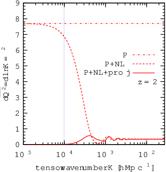
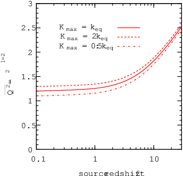
Fig. 2 gives an example (at ) of the contribution to the rms of the quadrupole per logarithmic interval of the tensor wavenumber . On subhorizon scales, the nonlinear mode-coupling effects partially cancel with the prediction from the primordial bispectrum alone. The constant limit for large reflects that each tensor mode induces the same cumulative effect (as evident from the limit in Fig. 1) on small-scale galaxy quadrupole from its horizon re-entry to damp-out, as long as . On the other hand, the projection effects kick in on superhorizon scales to cancel the primordial contribution, and hence ensure infrared-safety (without projection, the quadrupole will be proportional to superhorizon -folds). Therefore, the residual quadrupole from the full result is dramatically smaller. Fig. 3 shows the variance of the quadrupole as a function of the galaxy redshift. We truncate the tensor wavenumber at , but also show that a factor-of-two variation of that choice only modifies the result marginally. Over a wide range of redshifts () accessible to galaxy surveys the variance is .
VIII Conclusion
In this paper, we have derived the quadrupolar asymmetry imprinted on the galaxy (or other tracers of the matter) power spectrum due to long-wavelength tensor perturbations in single-field slow-roll (SFSR) inflation. We have considered the case of a scale hierarchy between the matter inhomogeneities of interest and the tensor perturbations, so the power quadrupole can be measured from many local volumes, across each of which the tensor perturbation marginally varies.
The observed quadrupole is the sum of three contributions: (1) A primordial quadrupole is imprinted at the end of inflation from a primordial curvature-curvature-tensor bispectrum, satisfying the squeezed-limit consistency relation. (2) An extra quadrupole develops during post-inflationary evolution, because matter clusters in the anisotropic background due to the long-wavelength tensor modes. This is a cosmic-scale analogy of the intrinsic alignment of galaxies due to tensor perturbations [18]. (3) A third contribution arises from projection into observed coordinates, which are defined by the observed redshift and the apparent angular position of the source. Unlike the amplitude of the primordial quadrupole due to tensor modes, which is sensitive to superhorizon -folds, the sum of the three contributions to observable effects is insensitive to tensor modes that are superhorizon today. We therefore conclude that the squeezed-limit consistency relations for primordial bispectra guarantee that superhorizon perturbations generated by SFSR inflation have no observable consequences on subhorizon physics. The residual effects are due to modes that are subhorizon or are undergoing horizon re-entry today. We have thus quantified in terms of precisely defined observables the magnitude of the observable quadrupole in the matter power spectrum suggested in Ref. [44].
With the current constraint on the inflationary tensor amplitude, the power quadrupole on scales is in single-field slow-roll inflation. On smaller scales the amount is expected to differ, but not significantly. Given the plenty of “real-world” complications such as redshift-space distortion and nonlinear evolution of matter perturbations, the imprints from tensors are beyond the reach of current large-scale-structure surveys. Nominally, this signal is an order of magnitude larger than the tensor-mode signals induced in the angular power spectra of galaxy clustering [58] and shear [18] through projection effects. Still, with future galaxy and 21-cm surveys, the quadrupolar power asymmetry might eventually provide a competitive probe of tensor modes from large-scale-structure surveys. Moreover, detection of the power asymmetry does not necessarily require a full-sky survey, as the overall signal-to-noise depends on the three-dimensional survey volume. Therefore, high-redshift accessibility can compensate for a moderate angular coverage.
If an inflation model violates the consistency relation Eq. (3), e.g. by having a different scaling law with respect to (preferably redder for phenomenological interest), then the infrared-safety of the observed power quadrupole will not hold. Such a scenario may predict a large quadrupole due to the abundance of superhorizon tensor modes, and hence will be subject to stringent constraints from observations. Conversely, detection of a large quadrupolar asymmetry in the galaxy power spectrum, beyond the level predicted in this work, would rule out single-field slow-roll inflation.
Acknowledgements.
We thank Fabian Schmidt for useful discussions and comments on an earlier draft. L.D. is grateful for the support of the William Gardner Fellowship. This work was supported by DoE SC-0008108 and NASA NNX12AE86G.Appendix A Primordial scalar two-point correlation in the presence of tensor
The primordial two-point correlation function for the scalar potential is the inverse Fourier-transform of Eq. (4),
| (38) | |||||
where we define and . For the second equality, the first term is the homogeneous and isotropic correlation in the absence of . For the second term, we plug in . Changing to and , we have
| (39) |
The integral fixes , and is just a number. Moreover, under the assumption we have the Taylor expansion,
| (40) |
because . We then integrate out and to obtain
| (41) |
In the last line, we have used the definition of the Fourier decomposition for . Together with the homogeneous/isotropic term in Eq. (38), this gives Eq. (5).
Appendix B Einstein and fluid equations
Here we present some key results in deriving the Einstein equations and the fluid equations in the Poisson gauge. We treat scalar/matter perturbations as independent small parameters from tensor perturbations, and at second-order we only keep their cross terms. We consistently assume that there is no primordial vector perturbations; thus, and are .
The Levi-Civita connection coefficients are given by
where we define and . The Ricci tensor is given by
| (42) | |||||
For a Universe dominated by non-relativistic matter with energy density , matter perturbations are parameterized by overdensity , and peculiar velocity (as measured by observers at fixed comoving position). Pressure and anisotropic stress can be neglected. The matter energy-stress tensor is given by
| (43) |
The Einstein equations for perturbations can be then obtained,
| (44) | |||
| (45) | |||
| (46) |
The fluid equations for perturbations can be derived from and by applying background evolution equations. They read
| (47) | |||||
| (48) |
Radiation needs to be added as an independent component when discussing the epoch of radiation-domination. We assume radiation is not coupled to matter (as for cold dark matter), but in the meantime has negligible higher moments (as it will if tightly coupled to a small amount of baryons). Then it can be described as a fluid with energy density (with perturbation ), pressure , and curl-free bulk velocity . Together with non-relativistic matter, the total energy-stress tensor reads,
| (49) |
With these equations, the corresponding Einstein equations and fluid equations can be derived straightforwardly.
Appendix C Equations for nonlinear corrections
A complete set of differential equations for the nonlinear corrections , , and can be obtained by extracting the second-order part of the Einstein equations, Eqs. (44) and (45) (take the divergence) and Eq. (46) (take the trace), and the fluid equations, Eqs. (47) and (48) (take the curl-free part). They can be simplified by applying the background evolution and the evolution equations for linear solutions. We collect them here,
| (50) | |||||
| (51) | |||||
| (52) | |||||
| (53) | |||||
| (54) |
We note that and drop out of these equations; as far as the matter overdensity is concerned, they can be ignored.
At nonlinear order, the difference between two scalar potentials does not vanish. Eliminating in terms of this symbol, we derive from Eq. (52),
| (55) |
Alternatively, we rewrite Eq. (51) and Eq. (54), respectively, as
| (56) | |||||
| (57) |
Eliminating and re-arranging the equation, we find
| (58) |
This is to be compared with Eq. (55) to give . The second source term in Eq. (55) is suppressed by a factor of , which is chosen to be small, relative to the first term. Therefore, we ignore this term afterwards.
Once is solved, and can be obtained from algebraic relations,
| (59) | |||||
| (60) |
following Eq. (50) and Eq. (51). When solving for , we also ignore the term in Eq. (59); it does not grow over time, and hence becomes negligible at late times when .
Eq. (IV.2) can be solved by the Green’s function. Two independent solutions to the homogeneous part of (where denotes the source term) includes a constant solution and a decaying one . The retarded Green’s function,
| (61) |
is then constructed from those two solutions. With null initial condition imposed, the solution for is
| (62) |
Appendix D Alternative derivation using Lagrangian coordinates
In this Appendix we provide an alternative derivation, using Lagrangian coordinates for a collection of freely-falling particles, of Eq. (14).
The matter distribution can be visualized as a collection of a huge number of non-relativistic matter particles of equal masses that fill the space. For collisionless matter, one can then track the position of individual particle—i.e., the Lagrangian coordinate—along the geodesic.
Consider a particle at comoving position at early times (). Let be the comoving displacement of that particle with respect to its initial position at any later time . The matter overdensity arises because the Lagrangian volume element differs from point to point, and we have
| (63) |
where is the overdensity at initial time. Note that keeping terms linear in suffices; since does not deflect comoving massive particles, , and terms higher-order in are at least , which are consistently ignored throughout this paper.
The 4-displacement can be solved from the geodesic equation,
| (64) |
where is the proper time. The ’s are calculated from Eq. (1). The geodesic equation must be supplemented by the equation describing how the matter distribution generates the gravitational potential . On subhorizon scales , the Poisson equation,
| (65) |
does the job. The tensor perturbation enters the left-hand side because the Poisson equation holds only in a “locally Newtonian” frame where is not felt. This is also validated by the subhorizon limit of Eq. (44). Furthermore, in the Newtonian limit we always assume .
Given the evolution of in Eq. (9), Eqs. (64) and (65) can be solved perturbatively. Following the spirit of Sec. IV, we keep the terms and linear in , as well as terms of , but not terms quadratic in or in potential/displacement. We split solutions into a linear part in the absence of , and a nonlinear correction of . In analogy to the notation of Sec. IV, we write and .
D.1 Linear solutions in the absence of tensor
The linear solutions can be obtained by taking . In order to solve for , setting suffices. The geodesic equation gives
| (66) |
Taking the divergence, and supplemented with the Poisson equation at linear order, we have
| (67) | |||||
| (68) |
which combine to give
| (69) |
Ignoring the decaying solution, we find constant, and hence is constant over time. From Eq. (68) and the time component of Eq. (64), we then find
| (70) |
D.2 Nonlinear corrections due to tensor
Since , it turns out that when solving for we can still identify . Then we can take the part of the spatial geodesic equation,
| (71) |
to obtain
| (72) |
where we have used to simplify. We then take the divergence, and use and to obtain
| (73) |
The part of the Poisson equation is
| (74) |
We then combine Eq. (73) and Eq. (74) to eliminate , and obtain
| (75) |
or in terms of conformal time,
| (76) |
The most general solution can be written as
| (77) |
where solves the homogeneous part of Eq. (76), while is a special solution that solves the full equation but vanishes at .
The homogeneous part of Eq. (76) has two independent solutions, and . Obviously, has to be . In fact, it has to be the unique solution for the case of infinite tensor wavelength, and . In that case, the same derivation to conclude constant from Eq. (69) leads to constant, and hence . From the initial condition , it must be that for infinite tensor wavelength, and hence,
| (78) |
To find for finite tensor wavelength, we construct the retarded Green’s function,
| (79) |
and then find
| (80) | |||||
where we define the function
| (81) |
Combining all the results, we are able to write (in Fourier space)
| (82) |
given the linear-extrapolation factor in the subhorizon limit . The right hand side can be simply evaluated at the initial location even if the test particle has moved by ; the difference made to is and hence can be ignored. For the subhorizon density modes that we are considering here, , and Eq. (82) exactly agrees with Eq. (14), given a correspondence between here and in Eq. (15):
| (83) |
where in the subhorizon limit .
With we have calculated in this Section, we can rewrite the fractional density perturbation in Eq. (14) as
| (84) |
and the corresponding matter power spectrum in the local coordinate Eq. (28) as
| (85) |
Finally, these changes are translated to the quadrupole in the observed power spectrum Eq. (33) as
| (86) |
We further re-arrange the quadrupole moments as
| (87) |
The third term in the parenthesis takes into account the projection effect, as it is the observed shear component including the metric shear [17, 18, 61] that arises from the transformation between local and global coordinates. That is, the third term is the quadrupole observed from a galaxy power spectrum which is isotropic in the local frame. Therefore, the first two terms should be interpreted as the “tidal effect” from the long-wavelength tensor mode to the locally observed matter power spectrum at the time when observed galaxies emitted photons.
Appendix E Galaxy overdensity in observed coordinates
Since the number of galaxies is conserved in whatever coordinates one uses, we can relate number density measured in the comoving FRW coordinates to that measured in observed coordinates through
| (88) |
where the Jacobian determinant is unity for traceless . We then define galaxy overdensities in both coordinates w.r.t. the average number density as expected from the homogeneous background cosmology,
| (89) | |||||
| (90) |
We can calculate , where can be measured for a specific galaxy sample. Besides, we have . Combining all the pieces, we find
| (91) |
which is Eq. (25).
Appendix F Local galaxy power spectrum in observed coordinates
The galaxy power spectrum on small scales can be written as
| (92) |
Inside the integral, we correlate two points and separated by with midpoint , so that . Assume that is small compared to both (the distance from the observer to the galaxy) and the variation scale of tensor perturbations .
Next, we apply Eq. (26), together with
| (93) |
In particular, for the term in Eq. (26), we expand to linear order in ,
| (94) |
as needed to find a quadrupole in the local power spectrum55 5 The higher-order terms in the expansion, are negligibly small and give higher-order multipoles. where and are to be computed at the midpoint . These can be recast in Fourier space, where we trade the separation (not the midpoint ) for the conjugated wavevector ,
| (95) |
On the other hand, the term can be just evaluated at the midpoint , since the correction starts only at quadratic order in .
Whenever a term is explicitly multiplied by a quantity first-order in , we can plug in the zeroth-order isotropic matter power spectrum , which does not depend on from statistical homogeneity in the absence of tensor perturbations. Then we are able to combine Eq. (26) and Eq. (95) to derive
| (96) | |||||
This gives Eq. (27). It is understood that background quantities (e.g. and ) and linear-order quantities in (e.g. and ) are computed at the midpoint , whose values are representative across the local volume.
Appendix G Calculation of the galaxy power quadrupole from long-wavelength tensor perturbations
Following the formalism of Ref. [19], we expand the tensor perturbation field (at primordial time) in terms of total-angular-momentum (TAM) waves,
| (97) |
From the Fourier-space power spectrum, Eq. (36), the TAM coefficients will satisfy
| (98) |
The quadrupole tensor measured at from a single TAM mode of wavenumber and total-angular-momentum and , analogous to Eq. (33), can be expanded in terms of tensor spherical harmonics,
| (99) |
where the direction on the sky is exactly the direction of as measured from the observer, and the redshift corresponds to the comoving distance assuming a background cosmology. Then in Eq. (VII), , where we sum over the five types of tensor spherical harmonics.
Below we present the explicit expressions for . First, we define coefficients,
| (100) | |||||
| (101) | |||||
| (102) |
which correspond to primordial, nonlinear mode-coupling, and projection effects, respectively. We then have
| (103) | |||||
| (104) | |||||
| (105) |
from -type TAM modes, and
| (106) | |||||
| (107) |
from -type TAM modes. Here is the comoving distance to the source, and the radial functions are given in Eqs. (22), (24), and (25) of Ref.[59]. Finally, terms involving components of , which can be calculated from Eqs. (23) and (24), are given by
| (108) | |||||
| (109) | |||||
| (110) | |||||
| (111) | |||||
| (112) | |||||
| (113) |
where we define line-of-sight integrals,
| (114) | |||||
| (115) | |||||
| (116) |
References
- [1] P. A. R. Ade et al. [Planck Collaboration], arXiv:1303.5082 [astro-ph.CO].
- [2] A. H. Guth and S. Y. Pi, Phys. Rev. Lett. 49, 1110 (1982).
- [3] J. M. Bardeen, P. J. Steinhardt and M. S. Turner, Phys. Rev. D 28, 679 (1983).
- [4] S. W. Hawking, Phys. Lett. B 115, 295 (1982).
- [5] A. D. Linde, Phys. Lett. B 108, 389 (1982).
- [6] V. F. Mukhanov and G. V. Chibisov, JETP Lett. 33, 532 (1981) [Pisma Zh. Eksp. Teor. Fiz. 33, 549 (1981)].
- [7] L. F. Abbott and M. B. Wise, Nucl. Phys. B 244, 541 (1984).
- [8] V. A. Rubakov, M. V. Sazhin and A. V. Veryaskin, Phys. Lett. B 115, 189 (1982).
- [9] R. Fabbri and M. d. Pollock, Phys. Lett. B 125, 445 (1983).
- [10] A. A. Starobinsky, JETP Lett. 30, 682 (1979) [Pisma Zh. Eksp. Teor. Fiz. 30, 719 (1979)].
- [11] M. Kamionkowski, A. Kosowsky and A. Stebbins, Phys. Rev. Lett. 78, 2058 (1997) [astro-ph/9609132].
- [12] U. Seljak and M. Zaldarriaga, Phys. Rev. Lett. 78, 2054 (1997) [astro-ph/9609169].
- [13] S. Kawamura, T. Nakamura, M. Ando, N. Seto, K. Tsubono, K. Numata, R. Takahashi and S. Nagano et al., Class. Quant. Grav. 23, S125 (2006).
- [14] T. L. Smith, M. Kamionkowski and A. Cooray, Phys. Rev. D 73, 023504 (2006) [astro-ph/0506422].
- [15] T. L. Smith, M. Kamionkowski and A. Cooray, Phys. Rev. D 78, 083525 (2008) [arXiv:0802.1530 [astro-ph]].
- [16] S. Chongchitnan and G. Efstathiou, Phys. Rev. D 73, 083511 (2006) [astro-ph/0602594].
- [17] S. Dodelson, E. Rozo and A. Stebbins, Phys. Rev. Lett. 91, 021301 (2003) [astro-ph/0301177].
- [18] F. Schmidt and D. Jeong, Phys. Rev. D 86, 083513 (2012) [arXiv:1205.1514 [astro-ph.CO]].
- [19] L. Dai, M. Kamionkowski and D. Jeong, Phys. Rev. D 86, 125013 (2012) [arXiv:1209.0761 [astro-ph.CO]].
- [20] A. Cooray, M. Kamionkowski and R. R. Caldwell, Phys. Rev. D 71, 123527 (2005) [astro-ph/0503002].
- [21] C. Li and A. Cooray, Phys. Rev. D 74, 023521 (2006) [astro-ph/0604179].
- [22] S. Dodelson, Phys. Rev. D 82, 023522 (2010) [arXiv:1001.5012 [astro-ph.CO]].
- [23] L. G. Book, M. Kamionkowski and T. Souradeep, Phys. Rev. D 85, 023010 (2012) [arXiv:1109.2910 [astro-ph.CO]].
- [24] U.-L. Pen, New Astron. 9, 417 (2004) [astro-ph/0305387].
- [25] K. W. Masui and U.-L. Pen, Phys. Rev. Lett. 105, 161302 (2010) [arXiv:1006.4181 [astro-ph.CO]].
- [26] L. Book, M. Kamionkowski and F. Schmidt, Phys. Rev. Lett. 108, 211301 (2012) [arXiv:1112.0567 [astro-ph.CO]].
- [27] A. R. Pullen and M. Kamionkowski, Phys. Rev. D 76, 103529 (2007) [arXiv:0709.1144 [astro-ph]].
- [28] D. Hanson and A. Lewis, Phys. Rev. D 80, 063004 (2009) [arXiv:0908.0963 [astro-ph.CO]].
- [29] S. Ando and M. Kamionkowski, Phys. Rev. Lett. 100, 071301 (2008) [arXiv:0711.0779 [astro-ph]].
- [30] A. R. Pullen and C. M. Hirata, JCAP 1005, 027 (2010) [arXiv:1003.0673 [astro-ph.CO]].
- [31] N. E. Groeneboom and H. K. Eriksen, Astrophys. J. 690, 1807 (2009) [arXiv:0807.2242 [astro-ph]].
- [32] C. L. Bennett, R. S. Hill, G. Hinshaw, D. Larson, K. M. Smith, J. Dunkley, B. Gold and M. Halpern et al., Astrophys. J. Suppl. 192, 17 (2011) [arXiv:1001.4758 [astro-ph.CO]].
- [33] P. A. R. Ade et al. [Planck Collaboration], arXiv:1303.5083 [astro-ph.CO].
- [34] D. Jeong and M. Kamionkowski, Phys. Rev. Lett. 108, 251301 (2012) [arXiv:1203.0302].
- [35] L. Dai, D. Jeong and M. Kamionkowski, arXiv:1302.1868 [astro-ph.CO].
- [36] J. M. Maldacena, JHEP 0305, 013 (2003) [astro-ph/0210603].
- [37] P. Creminelli and M. Zaldarriaga, JCAP 0410, 006 (2004) [astro-ph/0407059].
- [38] P. Creminelli, C. Pitrou and F. Vernizzi, JCAP 1111, 025 (2011) [arXiv:1109.1822 [astro-ph.CO]].
- [39] M. Gerstenlauer, A. Hebecker and G. Tasinato, JCAP 1106, 021 (2011) [arXiv:1102.0560 [astro-ph.CO]].
- [40] T. Tanaka and Y. Urakawa, JCAP 1105, 014 (2011) [arXiv:1103.1251 [astro-ph.CO]].
- [41] A. Lewis, JCAP 1206, 023 (2012) [arXiv:1204.5018 [astro-ph.CO]].
- [42] R. Flauger, D. Green and R. A. Porto, arXiv:1303.1430 [hep-th].
- [43] E. Pajer, F. Schmidt and M. Zaldarriaga, arXiv:1305.0824 [astro-ph.CO].
- [44] S. B. Giddings and M. S. Sloth, Phys. Rev. D 84, 063528 (2011) [arXiv:1104.0002 [hep-th]].
- [45] S. Brahma, E. Nelson and S. Shandera, in preparation.
- [46] M. H. Namjoo, H. Firouzjahi and M. Sasaki, Europhys. Lett. 101, 39001 (2013) [arXiv:1210.3692 [astro-ph.CO]].
- [47] E. Bertschinger, astro-ph/9503125.
- [48] L. Boubekeur, P. Creminelli, G. D’Amico, J. Norena and F. Vernizzi, JCAP 0908, 029 (2009) [arXiv:0906.0980 [astro-ph.CO]].
- [49] S. B. Giddings and M. S. Sloth, JCAP 1101, 023 (2011) [arXiv:1005.1056 [hep-th]].
- [50] N. Bartolo, S. Matarrese, O. Pantano and A. Riotto, Class. Quant. Grav. 27, 124009 (2010) [arXiv:1002.3759 [astro-ph.CO]].
- [51] D. Jeong, J. -O. Gong, H. Noh and J. -c. Hwang, Astrophys. J. 727, 22 (2011) [arXiv:1010.3489 [astro-ph.CO]].
- [52] J. Yoo, A. L. Fitzpatrick and M. Zaldarriaga, Phys. Rev. D 80, 083514 (2009) [arXiv:0907.0707 [astro-ph.CO]].
- [53] J. Yoo, Phys. Rev. D 82, 083508 (2010) [arXiv:1009.3021 [astro-ph.CO]].
- [54] A. Challinor and A. Lewis, Phys. Rev. D 84, 043516 (2011) [arXiv:1105.5292 [astro-ph.CO]].
- [55] C. Bonvin and R. Durrer, Phys. Rev. D 84, 063505 (2011) [arXiv:1105.5280 [astro-ph.CO]].
- [56] D. Jeong, F. Schmidt and C. M. Hirata, Phys. Rev. D 85, 023504 (2012) [arXiv:1107.5427 [astro-ph.CO]].
- [57] L. G. Book and E. E. Flanagan, Phys. Rev. D 83, 024024 (2011) [arXiv:1009.4192 [astro-ph.CO]].
- [58] D. Jeong and F. Schmidt, Phys. Rev. D 86, 083512 (2012) [arXiv:1205.1512 [astro-ph.CO]].
- [59] L. Dai, D. Jeong and M. Kamionkowski, Phys. Rev. D 87, 043504 (2013) [arXiv:1211.6110 [astro-ph.CO]].
- [60] E. Komatsu et al. [WMAP Collaboration], Astrophys. J. Suppl. 192, 18 (2011) [arXiv:1001.4538].
- [61] F. Schmidt and D. Jeong, Phys. Rev. D 86, 083527 (2012) [arXiv:1204.3625 [astro-ph.CO]].